Bogoliubov Theory

Bogoliubov theory describes small quantum fluctuations around a mean-field background by retaining the Hamiltonian through quadratic order and then finding canonical operators that diagonalize that quadratic form. The new operators create quasiparticles: normal modes that are coherent mixtures of particles and holes in the original basis.

Two logically distinct steps are often given the same name:

1. The Bogoliubov approximation chooses a background, expands the interacting Hamiltonian in fluctuations, and neglects cubic and higher fluctuation terms.
2. A Bogoliubov transformation is an exact linear canonical change of creation and annihilation operators for the resulting quadratic Hamiltonian.

The first step is approximate and needs a control parameter. The second is algebraically exact once the quadratic Hamiltonian has been specified. Keeping that distinction visible prevents a successful diagonalization from being mistaken for a proof that the original interacting model is weakly correlated.

For bosons, the transformation preserves commutators through an indefinite particle–hole metric. It is paraunitary rather than ordinarily unitary in Nambu space. That minus sign is responsible for hyperbolic normalization, squeezed vacua, positive- and negative-norm mode pairs, and the possibility of complex frequencies when the chosen background is dynamically unstable.

Canonical Scope

This page is the canonical home for:

• quadratic bosonic Hamiltonians with normal and anomalous terms;
• Nambu doubling and its constant-term bookkeeping;
• bosonic canonical and paraunitary transformations;
• the generalized eigenvalue problem and particle–hole metric;
• energetic, dynamical, and zero-mode stability diagnostics;
• exact one-mode squeezing as the elementary example;
• the uniform dilute Bose-gas spectrum and quasiparticle amplitudes;
• ultraviolet structure of the quadratic vacuum correction;
• inhomogeneous Bogoliubov–de Gennes equations around a condensate;
• the contrast between bosonic and fermionic transformations;
• number-conserving interpretations and limits of the approximation.

Gross–Pitaevskii Equation owns the condensate background and its nonlinear dynamics. Weakly Interacting Bose Gas Preview owns the physical overview of depletion, the Lee–Huang–Yang correction, the structure factor, and superfluidity. Goldstone Modes in Many-Body Systems explains why a neutral-superfluid phonon is symmetry-protected and places it in the nonrelativistic counting theorem. Phonons as Many-Body Excitations owns the distinct quantization of atomic lattice vibrations. Polarons Preview uses the resulting Bogoliubov density modes as the host excitations dressing a mobile impurity. Squeezed States as Entangled Modes owns continuous-variable squeezing and mode entanglement. BCS Mean-Field Theory owns the Cooper instability, self-consistent gap equation, and superconducting interpretation of fermionic quasiparticles. Quasiparticles Overview owns the broader concept beyond quadratic canonical diagonalization.

Why Anomalous Terms Appear

Suppose an interacting bosonic Hamiltonian is expanded around a classical field or other mean-field reference. For a condensate,

$$\hat\psi = \Phi + \delta\hat\psi.$$

The Hamiltonian becomes an expansion in fluctuation operators:

$$\hat H = H^{[0]} + \hat H^{[1]} + \hat H^{[2]} + \hat H^{[3]} + \cdots.$$

The terms have distinct roles:

Fluctuation order	Interpretation
zero	mean-field energy
one	vanishes when the background is stationary
two	independent normal modes after canonical diagonalization
three and higher	quasiparticle interactions and corrections beyond leading order

The quadratic part generally contains both number-conserving bilinears,

$$\hat a_i^\dagger\hat a_j,$$

and anomalous pair terms,

$$\hat a_i^\dagger\hat a_j^\dagger, \qquad \hat a_j\hat a_i.$$

The anomalous terms mean that bare-particle number is not conserved by the truncated fluctuation Hamiltonian. They do not imply that the microscopic Hamiltonian violates total particle-number conservation. They arise because the background acts as a phase and particle reservoir in a symmetry-breaking description, or because condensate particles are transferred into and out of the noncondensed sector in a number-conserving formulation.

General Quadratic Bosonic Hamiltonian

For $M$ bosonic modes, write

$$\begin{aligned} \hat H_2 = E_{\mathrm c} &+ \sum_{i,j} A_{ij}\hat a_i^\dagger\hat a_j \\ &+ \frac{1}{2} \sum_{i,j} \left( B_{ij}\hat a_i^\dagger\hat a_j^\dagger + B_{ij}^*\hat a_j\hat a_i \right). \end{aligned}$$

Hermiticity and bosonic commutation require

$$A = A^\dagger, \qquad B = B^T.$$

The symmetry of $B$ reflects

$$\hat a_i^\dagger\hat a_j^\dagger = \hat a_j^\dagger\hat a_i^\dagger.$$

An antisymmetric part would multiply a vanishing bosonic pair operator and carries no physical information.

Nambu vector

Introduce

$$\hat\Gamma = \begin{pmatrix} \hat{\mathbf a} \\ \hat{\mathbf a}^\dagger \end{pmatrix},$$

where

$$\hat{\mathbf a} = \begin{pmatrix} \hat a_1 \\ \vdots \\ \hat a_M \end{pmatrix}.$$

Define the Hermitian bosonic Nambu matrix

$$\mathcal H_{\mathrm B} = \begin{pmatrix} A & B \\ B^* & A^T \end{pmatrix}.$$

Then

$$\hat H_2 = E_{\mathrm c} - \frac{1}{2}\operatorname{Tr}A + \frac{1}{2} \hat\Gamma^\dagger \mathcal H_{\mathrm B} \hat\Gamma.$$

The subtraction is essential. Nambu notation writes particle and hole components together, so the lower block reproduces the normal term plus a commutator constant:

$$\hat{\mathbf a} A^T \hat{\mathbf a}^\dagger = \operatorname{Tr}A + \hat{\mathbf a}^\dagger A \hat{\mathbf a}.$$

Forgetting the factor $1/2$ or the trace subtraction double counts degrees of freedom and shifts the vacuum energy incorrectly.

The Bosonic Particle–Hole Metric

The Nambu components do not obey a positive-definite canonical algebra. Instead,

$$[ \hat\Gamma_\alpha, \hat\Gamma_\beta^\dagger ] = (\Sigma_z)_{\alpha\beta},$$

with

$$\Sigma_z = \begin{pmatrix} I_M & 0 \\ 0 & -I_M \end{pmatrix}.$$

The minus sign comes from

$$[ \hat a_i^\dagger, \hat a_j ] = -\delta_{ij}.$$

It is not an optional convention. It determines which linear transformations preserve the canonical commutators and which eigenvalue problem governs the dynamics.

The Heisenberg equation is

$$i\hbar\partial_t\hat\Gamma = \Sigma_z \mathcal H_{\mathrm B} \hat\Gamma.$$

Thus the dynamical matrix is

$$\mathcal D_{\mathrm B} = \Sigma_z\mathcal H_{\mathrm B}.$$

Although $\mathcal H_{\mathrm B}$ is Hermitian, $\mathcal D_{\mathrm B}$ is generally not Hermitian in the ordinary Euclidean inner product. It satisfies

$$\mathcal D_{\mathrm B}^\dagger = \Sigma_z \mathcal D_{\mathrm B} \Sigma_z,$$

which is a particle–hole metric relation. Diagonalizing $\mathcal H_{\mathrm B}$ as though it were an ordinary one-particle Hamiltonian therefore gives the wrong normal-mode problem.

Bosonic Canonical Transformation

Let

$$\hat\Gamma = T\hat\Gamma_\beta, \qquad \hat\Gamma_\beta = \begin{pmatrix} \hat{\boldsymbol\beta} \\ \hat{\boldsymbol\beta}^\dagger \end{pmatrix}.$$

To preserve commutators, $T$ must satisfy

$$T\Sigma_zT^\dagger = \Sigma_z.$$

For an invertible square transformation, this is equivalent to

$$T^\dagger\Sigma_zT = \Sigma_z,$$

and

$$T^{-1} = \Sigma_zT^\dagger\Sigma_z.$$

Such a matrix is called paraunitary. A useful block form is

$$T = \begin{pmatrix} U & V^* \\ V & U^* \end{pmatrix},$$

corresponding to

$$\hat{\mathbf a} = U\hat{\boldsymbol\beta} + V^*\hat{\boldsymbol\beta}^\dagger.$$

The block conditions include

$$U^\dagger U - V^\dagger V = I,$$

and

$$U^TV - V^TU = 0.$$

Signs assigned to $V$ differ across references. The invariant content is the preserved commutator metric, not one preferred sign convention.

For one real pair of amplitudes, the normalization is

$$u^2-v^2 = 1.$$

It can be parameterized by

$$u = \cosh r, \qquad v = \sinh r.$$

This hyperbolic geometry is the algebraic reason bosonic Bogoliubov vacua are squeezed states.

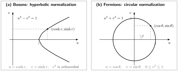
Real-coefficient slices of the canonical constraints. Bosons preserve $u^2-v^2=1$, giving a hyperbola and unbounded $v^2$. Fermions preserve $u^2+v^2=1$, giving a circle and $0\leq v^2\leq1$. Complex multimode transformations obey the corresponding matrix conditions.

Generalized Eigenvalue Problem

The normal modes solve

$$\mathcal D_{\mathrm B}w_\nu = E_\nu w_\nu,$$

or equivalently

$$\mathcal H_{\mathrm B}w_\nu = E_\nu\Sigma_z w_\nu.$$

For a stable positive-energy mode, choose the metric normalization

$$w_\nu^\dagger \Sigma_z w_\mu = \delta_{\nu\mu}.$$

If

$$w_\nu = \begin{pmatrix} u_\nu \\ v_\nu \end{pmatrix},$$

then

$$u_\nu^\dagger u_\nu - v_\nu^\dagger v_\nu = 1.$$

Particle–hole symmetry generates a partner

$$\widetilde w_\nu = \Sigma_x w_\nu^*,$$

where

$$\Sigma_x = \begin{pmatrix} 0 & I_M \\ I_M & 0 \end{pmatrix}.$$

The partner has eigenvalue $-E_\nu^*$ and opposite metric norm. Positive and negative branches are therefore Nambu partners, not two independent sets of physical bosonic excitations.

When a complete stable paraunitary basis exists,

$$T^\dagger \mathcal H_{\mathrm B} T = \begin{pmatrix} \mathcal E & 0 \\ 0 & \mathcal E \end{pmatrix},$$

with

$$\mathcal E = \operatorname{diag}(E_1,\ldots,E_M), \qquad E_\nu>0.$$

The Hamiltonian becomes

$$\hat H_2 = E_{\mathrm{vac}} + \sum_{\nu=1}^{M} E_\nu \hat\beta_\nu^\dagger\hat\beta_\nu,$$

where

$$E_{\mathrm{vac}} = E_{\mathrm c} - \frac{1}{2}\operatorname{Tr}A + \frac{1}{2} \sum_{\nu=1}^{M}E_\nu.$$

The vacuum shift is physical only after the same regulator and parameter matching used to define the quadratic model have been applied.

Stability Is More Than Real-Looking Algebra

Three ideas should be separated.

Energetic stability

An equilibrium background is energetically stable at quadratic order when the constrained second variation is nonnegative. For a finite bosonic system without zero modes, positive definiteness of $\mathcal H_{\mathrm B}$ is a strong sufficient condition for a conventional positive-energy diagonalization.

Dynamical stability

The linearized motion is dynamically stable when the frequencies are real and the evolution does not contain exponentially growing modes. A complex eigenvalue of

$$\Sigma_z\mathcal H_{\mathrm B}$$

produces exponential growth or decay. It is not the energy of a long-lived quasiparticle.

Negative-energy and zero modes

A real spectrum can still contain a negative-energy mode relative to the chosen frame or constraint. Such a mode signals energetic instability even when isolated linear dynamics oscillates.

Continuous symmetries can produce zero modes. Their metric norm may vanish, and the dynamical matrix can require generalized eigenvectors rather than an ordinary normalized basis. Zero modes must be treated separately; dividing by their norm or counting both Nambu partners as ordinary oscillators is invalid.

In rotating systems, the relevant energy is often

$$E - \Omega L_z.$$

A mode that is positive in the laboratory frame can become negative in the rotating frame. Stability claims must therefore state the frame and constraints.

Single-Mode Squeezing Example

Consider

$$\hat H = A\hat a^\dagger\hat a + \frac{B}{2} \left( \hat a^{\dagger 2} + \hat a^2 \right),$$

where $A$ and $B$ are real. Use

$$\hat a = \cosh r\,\hat b - \sinh r\,\hat b^\dagger.$$

The anomalous terms vanish when

$$\tanh 2r = \frac{B}{A}.$$

A real $r$ exists for

$$A > |B|.$$

The excitation energy is

$$E = \sqrt{A^2-B^2},$$

and the diagonal Hamiltonian is

$$\hat H = E\hat b^\dagger\hat b + \frac{E-A}{2}.$$

The new vacuum is lower in energy than the original empty-$a$ vacuum when $B\ne0$. It contains

$$\langle0_b| \hat a^\dagger\hat a |0_b\rangle = \sinh^2r.$$

At $A=|B|$, the mode softens to zero. For $A<|B|$, $E$ is imaginary and the quadratic form is unbounded along one quadrature. Writing a formal complex squeezing parameter does not turn that instability into a stable oscillator.

Uniform Dilute Bose Gas

The canonical physical application is a homogeneous, weakly repulsive Bose gas. In a volume $V$,

$$\hat H = \sum_{\mathbf k} \epsilon_k \hat a_{\mathbf k}^\dagger \hat a_{\mathbf k} + \frac{g}{2V} \sum_{\mathbf k,\mathbf k',\mathbf q} \hat a_{\mathbf k+\mathbf q}^\dagger \hat a_{\mathbf k'-\mathbf q}^\dagger \hat a_{\mathbf k'} \hat a_{\mathbf k},$$

where

$$\epsilon_k = \frac{\hbar^2k^2}{2m}, \qquad g = \frac{4\pi\hbar^2a_s}{m}.$$

Work with

$$\hat K = \hat H - \mu\hat N.$$

For a macroscopically occupied zero-momentum mode, set

$$\hat a_{\mathbf0} \approx \sqrt{N_0}$$

in the symmetry-breaking organization and retain terms through quadratic order in nonzero-momentum operators. Stationarity fixes

$$\mu = gn_0, \qquad n_0 = \frac{N_0}{V}.$$

The quadratic grand Hamiltonian is

$$\begin{aligned} \hat K_2 = \sum_{\mathbf k\ne\mathbf0} \Bigg[ &(\epsilon_k+gn_0) \hat a_{\mathbf k}^\dagger \hat a_{\mathbf k} \\ &+ \frac{gn_0}{2} \left( \hat a_{\mathbf k}^\dagger \hat a_{-\mathbf k}^\dagger + \hat a_{\mathbf k} \hat a_{-\mathbf k} \right) \Bigg]. \end{aligned}$$

Opposite momenta form independent Nambu sectors because the background is translation invariant.

Pairwise Diagonalization

Choose the convention

$$\hat a_{\mathbf k} = u_k\hat b_{\mathbf k} - v_k\hat b_{-\mathbf k}^\dagger,$$

with real, even coefficients

$$u_{-k} = u_k, \qquad v_{-k} = v_k.$$

Commutator preservation requires

$$u_k^2-v_k^2 = 1.$$

For

$$A_k = \epsilon_k+gn_0, \qquad B_k = gn_0,$$

the anomalous terms vanish when

$$\tanh 2r_k = \frac{B_k}{A_k}, \qquad u_k = \cosh r_k, \qquad v_k = \sinh r_k.$$

The positive excitation energy is

$$E_k = \sqrt{A_k^2-B_k^2} = \sqrt{ \epsilon_k (\epsilon_k+2gn_0) }.$$

The amplitudes are

$$u_k^2 = \frac{1}{2} \left( \frac{\epsilon_k+gn_0}{E_k} + 1 \right),$$ $$v_k^2 = \frac{1}{2} \left( \frac{\epsilon_k+gn_0}{E_k} - 1 \right),$$

and

$$u_kv_k = \frac{gn_0}{2E_k}.$$

The diagonal form is

$$\hat K_2 = \frac{1}{2} \sum_{\mathbf k\ne\mathbf0} \left( E_k-A_k \right) + \sum_{\mathbf k\ne\mathbf0} E_k \hat b_{\mathbf k}^\dagger \hat b_{\mathbf k}.$$

The sum over all nonzero $\mathbf k$ is correct here because the explicit factor $1/2$ in the vacuum term compensates Nambu pairing. An alternative derivation may sum only over one representative from each pair $\{\mathbf k,-\mathbf k\}$. Mixing those conventions creates a factor-of-two error.

Phonon and Particle Regimes

At long wavelength,

$$E_k \approx \hbar c k,$$

where

$$c = \sqrt{\frac{gn_0}{m}}.$$

The quasiparticle is a collective phonon. In this limit,

$$u_k \approx v_k \approx \sqrt{ \frac{mc}{2\hbar k} },$$

so neither the particle nor the hole component is a small correction.

The combinations

$$(u_k-v_k)^2 = \frac{\epsilon_k}{E_k},$$

and

$$(u_k+v_k)^2 = \frac{\epsilon_k+2gn_0}{E_k}$$

separate density-like and phase-like fluctuation weights in this convention. At small $k$, density fluctuations are suppressed while phase fluctuations are enhanced.

At high momentum within the contact theory’s range of validity,

$$E_k = \epsilon_k + gn_0 + O(\epsilon_k^{-1}),$$ $$u_k \longrightarrow 1, \qquad v_k \approx \frac{gn_0}{2\epsilon_k}.$$

The mode becomes particle-like. The crossover occurs at

$$k\xi \sim 1,$$

where

$$\xi = \frac{\hbar}{\sqrt{2mgn_0}}.$$

The existing dispersion figure and the thermodynamic consequences are collected in Weakly Interacting Bose Gas Preview.

The Quasiparticle Vacuum

Define

$$\hat b_{\mathbf k} |0_b\rangle = 0$$

for every nonzero momentum. The inverse transformation is

$$\hat b_{\mathbf k} = u_k\hat a_{\mathbf k} + v_k\hat a_{-\mathbf k}^\dagger.$$

For one representative of each pair,

$$|0_b\rangle \propto \prod_{\mathbf k>0} \exp\!\left[ -\frac{v_k}{u_k} \hat a_{\mathbf k}^\dagger \hat a_{-\mathbf k}^\dagger \right] |0_a\rangle.$$

It is a two-mode squeezed vacuum in the bare-particle basis. Its leading contractions are

$$\langle0_b| \hat a_{\mathbf k}^\dagger \hat a_{\mathbf k} |0_b\rangle = v_k^2,$$

and

$$\langle0_b| \hat a_{\mathbf k} \hat a_{-\mathbf k} |0_b\rangle = -u_kv_k.$$

Thus a quasiparticle vacuum need not be empty of particles. Conversely, one bare atom is not generally one normal-mode excitation.

At temperature $T$,

$$n_{\mathrm B}(E_k) = \frac{1}{ e^{\beta E_k}-1 },$$

and

$$\begin{aligned} \langle \hat a_{\mathbf k}^\dagger \hat a_{\mathbf k} \rangle ={}& (u_k^2+v_k^2) n_{\mathrm B}(E_k) \\ &+ v_k^2. \end{aligned}$$

The first term is thermal quasiparticle occupation mapped back to particles; the second is zero-temperature quantum depletion.

For infinitely many modes, a canonical algebra transformation need not be implemented by a unitary operator on the original Fock representation. A sufficient finite-depletion condition is

$$\sum_\nu \|v_\nu\|^2 < \infty.$$

In continuum problems, volume limits, infrared behavior, and ultraviolet matching must therefore be stated before two vacua are declared to belong to the same Hilbert-space representation.

Vacuum Energy and Ultraviolet Matching

For the contact gas, the formal zero-point shift is

$$\Delta E_{\mathrm{zp}} = \frac{1}{2} \sum_{\mathbf k\ne\mathbf0} \left( E_k - \epsilon_k - gn_0 \right).$$

At large $k$,

$$E_k - \epsilon_k - gn_0 \sim - \frac{(gn_0)^2}{2\epsilon_k}.$$

The three-dimensional momentum integral is ultraviolet divergent. This is not a failure of the low-energy spectrum. It signals that a bare contact coefficient cannot be used simultaneously as a physical scattering amplitude without matching.

After expressing the coupling in terms of the physical scattering length, the leading regulated energy density may be organized as

$$\begin{aligned} \frac{E_0}{V} = \frac{gn^2}{2} + \frac{1}{2} \int\frac{d^3k}{(2\pi)^3} \Bigg[ &E_k - \epsilon_k - gn \\ &+ \frac{(gn)^2}{2\epsilon_k} \Bigg]. \end{aligned}$$

The counterterm cancels the displayed high-momentum asymptote. Evaluating the finite integral produces the Lee–Huang–Yang correction, whose canonical physical discussion remains in the weak-gas page. Normal ordering alone does not perform this coupling renormalization.

Inhomogeneous Bogoliubov–de Gennes Equations

Let $\Phi(\mathbf r)$ solve the stationary Gross–Pitaevskii equation,

$$\left[ -\frac{\hbar^2}{2m}\nabla^2 + V_{\mathrm{ext}} + g|\Phi|^2 \right]\Phi = \mu\Phi.$$

Perturb the time-dependent field as

$$\Psi(\mathbf r,t) = e^{-i\mu t/\hbar} \left[ \Phi(\mathbf r) + \delta\psi(\mathbf r,t) \right].$$

Use the mode ansatz

$$\delta\psi = u_\nu(\mathbf r) e^{-i\omega_\nu t} - v_\nu^*(\mathbf r) e^{i\omega_\nu t}.$$

Linearization gives

$$\begin{pmatrix} \mathcal L & g\Phi^2 \\ -g\Phi^{*2} & -\mathcal L^* \end{pmatrix} \begin{pmatrix} u_\nu \\ v_\nu \end{pmatrix} = \hbar\omega_\nu \begin{pmatrix} u_\nu \\ v_\nu \end{pmatrix},$$

where

$$\mathcal L = -\frac{\hbar^2}{2m}\nabla^2 + V_{\mathrm{ext}} - \mu + 2g|\Phi|^2.$$

The factor $2g|\Phi|^2$ in $\mathcal L$ and the anomalous coupling $g\Phi^2$ come from different derivatives of the cubic mean field. Replacing both by one Hartree shift destroys the gapless phase mode.

The bosonic norm is

$$\int d^3r\, \left( |u_\nu|^2 - |v_\nu|^2 \right) = 1$$

for a positive-norm mode. Distinct stable modes satisfy the corresponding metric orthogonality relation.

If $(u_\nu,v_\nu)^T$ has frequency $\omega_\nu$, then

$$\begin{pmatrix} v_\nu^* \\ u_\nu^* \end{pmatrix}$$

is the particle–hole partner with frequency $-\omega_\nu^*$.

Phase zero mode

Global phase invariance produces

$$\begin{pmatrix} u_0 \\ v_0 \end{pmatrix} \propto \begin{pmatrix} \Phi \\ -\Phi^* \end{pmatrix}.$$

Substitution gives

$$\omega_0 = 0.$$

Its metric norm vanishes:

$$\int d^3r\, \left( |\Phi|^2 - |\Phi|^2 \right) = 0.$$

This vector cannot be normalized as an ordinary quasiparticle. A complete treatment pairs it with a generalized number or phase direction, or projects the condensate mode out in a number-conserving construction.

Number-Conserving Formulations

The symmetry-breaking derivation assigns a classical amplitude to the condensate and allows the fluctuation Hamiltonian to exchange particles with that background. It is efficient, but an exact fixed-$N$ state obeys

$$\langle\hat\psi\rangle = 0.$$

Number-conserving approaches instead separate the condensate orbital from the orthogonal fluctuation field. Schematically,

$$\hat\psi = \hat a_0\phi_0 + \delta\hat\psi_\perp,$$

with

$$\int d^3r\, \phi_0^* \delta\hat\psi_\perp = 0.$$

Composite fluctuation operators transfer one particle between the condensate and orthogonal sectors while preserving total $N$. To leading order in small depletion, they reproduce the same physical positive-frequency spectrum as the broken-symmetry method.

The formulations differ in bookkeeping:

• broken symmetry makes the phase and anomalous averages explicit;
• number conservation keeps every state in one number sector;
• the condensate phase zero mode is handled differently;
• finite-$N$ corrections and projector terms become more visible in the number-conserving form.

Neither formalism licenses neglecting depletion. Both require the noncondensed population and higher fluctuation terms to remain controlled.

Fermionic Bogoliubov Preview

Fermionic pairing Hamiltonians also mix creation and annihilation operators, but anticommutation changes the canonical geometry. Consider one paired block,

$$\begin{aligned} \hat H_{\mathbf k} ={}& \xi_k \left( \hat c_{\mathbf k}^\dagger\hat c_{\mathbf k} + \hat c_{-\mathbf k}^\dagger\hat c_{-\mathbf k} \right) \\ &- \left( \Delta \hat c_{\mathbf k}^\dagger \hat c_{-\mathbf k}^\dagger + \Delta^* \hat c_{-\mathbf k} \hat c_{\mathbf k} \right). \end{aligned}$$

In the Nambu basis

$$\begin{pmatrix} \hat c_{\mathbf k} \\ \hat c_{-\mathbf k}^\dagger \end{pmatrix},$$

the corresponding Bogoliubov–de Gennes matrix can be written

$$\mathcal H_{\mathrm F}(\mathbf k) = \begin{pmatrix} \xi_k & -\Delta \\ -\Delta^* & -\xi_k \end{pmatrix}.$$

This matrix is Hermitian. Its eigenvalues are

$$\pm E_k, \qquad E_k = \sqrt{\xi_k^2+|\Delta|^2}.$$

A fermionic quasiparticle has the form

$$\hat\gamma_{\mathbf k} = u_k\hat c_{\mathbf k} - v_k\hat c_{-\mathbf k}^\dagger.$$

Anticommutator preservation requires

$$|u_k|^2 + |v_k|^2 = 1.$$

For real positive $\Delta$,

$$|u_k|^2 = \frac{1}{2} \left( 1+\frac{\xi_k}{E_k} \right),$$

and

$$|v_k|^2 = \frac{1}{2} \left( 1-\frac{\xi_k}{E_k} \right).$$

The transformation is a compact rotation rather than a hyperbolic squeeze. Fermionic occupation of one mode is bounded by Pauli exclusion, while bosonic $v^2$ can grow without bound as a mode softens.

The negative fermionic BdG branch is also a Nambu redundancy, not an independent negative-energy particle. The full BCS construction must additionally determine $\Delta$ self-consistently and account for constants, filling, symmetry, and the interaction cutoff. Those tasks are derived in BCS Mean-Field Theory.

Bosons and Fermions Compared

Feature	Bosons	Fermions
canonical algebra	commutator	anticommutator
pair matrix	symmetric	antisymmetric in complete labels
scalar normalization	$	u
Nambu transformation	paraunitary	unitary with particle–hole constraint
coefficient geometry	hyperbolic	circular
bare-mode occupation in vacuum	unbounded in principle	between zero and one
mode equation	generally non-Hermitian dynamical matrix	Hermitian BdG matrix in standard form
instability signal	complex frequency possible	self-consistent saddle may fail, but Hermitian block has real eigenvalues
conserved quantity in number-breaking form	quasiparticle description need not conserve bare $N$	fermion parity remains conserved

The shared phrase “Bogoliubov transformation” refers to preserving the appropriate canonical algebra. It does not mean that bosonic and fermionic Nambu problems have the same metric or stability theory.

What the Approximation Omits

Quasiparticle interactions

Cubic and quartic fluctuation terms produce scattering among quasiparticles, energy shifts, and finite lifetimes. Beliaev decay at low temperature and Landau damping at finite temperature are beyond a strictly quadratic Hamiltonian.

Self-consistent backreaction

If depletion is not negligible, the condensate equation and fluctuation spectrum must be solved with consistent normal and anomalous densities. Naive self-consistent closures can violate conservation laws or open an unphysical gap. “Self-consistent” is not by itself a guarantee of a conserving and gapless approximation.

Critical and low-dimensional fluctuations

Near a phase transition or in sufficiently low dimension, infrared fluctuations can invalidate expansion around one rigid order parameter. A formally gapless quadratic mode may make fluctuation integrals divergent, signaling the need for finite-size, algebraic-order, renormalization-group, or nonperturbative treatments.

Strong depletion and fragmentation

When no single mode dominates the one-body density matrix, a one-condensate Bogoliubov expansion is the wrong starting point. Strongly correlated lattice phases, Tonks–Girardeau gases, and fragmented condensates require different reference spaces.

Time-dependent backgrounds

For a time-dependent mean field, instantaneous eigenmodes need not evolve independently. The basis itself changes, positive- and negative-frequency components can mix, and nonadiabatic quasiparticle production can occur. Solving a static eigenproblem at each time is not automatically an exact time-evolution method.

Broader Applications

The same quadratic logic appears in:

• spin-wave theory and magnons after a Holstein–Primakoff expansion;
• harmonic fluctuations around ordered lattice phases;
• parametric amplifiers and squeezed light;
• BCS and Hartree–Fock–Bogoliubov theories;
• Jordan–Wigner solutions of paired fermion chains;
• nuclear pairing and quasiparticle random-phase methods;
• free quantum fields in different mode decompositions.

Each application supplies its own background, canonical algebra, constraints, and regulator. The transformation is a method, not a universal physical approximation independent of context.

Reliable Workflow

1. Specify the reference. State the condensate, saddle, ordered state, or pairing field.
2. State the constraint. Use $H$, $H-\mu N$, or the appropriate rotating-frame or constrained functional.
3. Check stationarity. Linear fluctuation terms must vanish for the claimed background.
4. Retain constants. Record Nambu factors, trace subtractions, and double-counting corrections.
5. Identify statistics. Enforce $B=B^T$ for bosons or the appropriate fermionic antisymmetry.
6. Solve the correct eigenproblem. Use $\Sigma_z\mathcal H_{\mathrm B}$ for bosonic dynamics.
7. Normalize with the correct metric. Check positive and negative Nambu partners.
8. Diagnose stability. Report complex, negative-energy, and zero modes separately.
9. Check convergence. Resolve infrared size dependence and ultraviolet cutoff dependence.
10. Estimate omitted terms. Quantify depletion, quasiparticle occupation, or interaction corrections.

Common Mistakes

Calling the quadratic truncation exact

The canonical transformation exactly diagonalizes $\hat H_2$. It does not restore the discarded $\hat H^{[3]}$, $\hat H^{[4]}$, and higher terms.

Diagonalizing the bosonic Nambu matrix ordinarily

Bosonic frequencies are eigenvalues of $\Sigma_z\mathcal H_{\mathrm B}$, not generally of $\mathcal H_{\mathrm B}$ itself.

Replacing the minus norm by a plus norm

For bosons, $|u|^2-|v|^2=1$. The plus sign belongs to fermionic anticommutation.

Counting both Nambu branches as particles

The negative branch is the particle–hole partner of the positive branch. Counting both doubles the physical modes and corrupts the zero-point energy.

Dropping the constant

Quadratic diagonalization changes the vacuum energy. The constant matters for ground-state energies, phase competition, and thermodynamic derivatives.

Interpreting an imaginary frequency as a quasiparticle energy

It is a dynamical instability rate of the assumed background.

Treating a zero mode as an ordinary normalized oscillator

Symmetry zero modes can have zero metric norm and require projectors or generalized eigenvectors.

Using a physical contact coupling without ultraviolet matching

The spectrum may be finite while the zero-point integral diverges. Coupling renormalization and normal ordering are different operations.

Equating quasiparticle number with particle number

A quasiparticle mixes creation and annihilation operators. Its vacuum already contains bare particles, and one quasiparticle need not add one atom.

Assuming broken symmetry is mandatory

Number-conserving formulations reproduce the leading spectrum without placing the exact state in a superposition of total particle numbers.

Exercises

Preserve the bosonic commutator

For two opposite-momentum modes, let

$$\hat a_{\mathbf k} = u\hat b_{\mathbf k} - v\hat b_{-\mathbf k}^\dagger,$$

and

$$\hat a_{-\mathbf k} = u\hat b_{-\mathbf k} - v\hat b_{\mathbf k}^\dagger,$$

with real $u,v$. Derive the canonical constraint and check the crossed commutator.

Solution

Using the $b$-mode algebra,

$$\begin{aligned} [ \hat a_{\mathbf k}, \hat a_{\mathbf k}^\dagger ] &= u^2 [ \hat b_{\mathbf k}, \hat b_{\mathbf k}^\dagger ] \\ &\quad+ v^2 [ \hat b_{-\mathbf k}^\dagger, \hat b_{-\mathbf k} ] \\ &= u^2-v^2. \end{aligned}$$

Therefore canonical normalization requires

$$u^2-v^2 = 1.$$

The crossed commutator is

$$\begin{aligned} [ \hat a_{\mathbf k}, \hat a_{-\mathbf k} ] ={}& -uv [ \hat b_{\mathbf k}, \hat b_{\mathbf k}^\dagger ] \\ &- uv [ \hat b_{-\mathbf k}^\dagger, \hat b_{-\mathbf k} ] \\ =&0. \end{aligned}$$

The second matrix condition is therefore also satisfied.

Diagonalize one squeezed mode

For

$$\hat H = A\hat a^\dagger\hat a + \frac{B}{2} \left( \hat a^{\dagger2} + \hat a^2 \right),$$

derive the coefficient of $\hat b^{\dagger2}+\hat b^2$ after the hyperbolic transformation and obtain the stability condition, energy, and vacuum shift.

Solution

Set

$$c = \cosh r, \qquad s = \sinh r, \qquad \hat a = c\hat b-s\hat b^\dagger.$$

The anomalous coefficient is

$$-Acs + \frac{B}{2} (c^2+s^2).$$

Using

$$2cs = \sinh2r, \qquad c^2+s^2 = \cosh2r,$$

it vanishes when

$$\tanh2r = \frac{B}{A}.$$

A real solution requires $|B|<A$. The remaining number coefficient is

$$E = \sqrt{A^2-B^2}.$$

Normal ordering gives

$$\hat H = E\hat b^\dagger\hat b + \frac{E-A}{2}.$$

At $|B|=A$ the mode is soft; beyond that point the frequency is imaginary.

Nambu trace subtraction

Starting from

$$\mathcal H_{\mathrm B} = \begin{pmatrix} A & B \\ B^* & A^T \end{pmatrix},$$

show why

$$\frac12 \hat\Gamma^\dagger \mathcal H_{\mathrm B} \hat\Gamma$$

contains an additional $\operatorname{Tr}A/2$ compared with the normally ordered quadratic Hamiltonian.

Solution

Expanding the Nambu bilinear gives

$$\begin{aligned} \frac12 \hat\Gamma^\dagger \mathcal H_{\mathrm B} \hat\Gamma ={}& \frac12 \hat{\mathbf a}^\dagger A \hat{\mathbf a} \\ &+ \frac12 \hat{\mathbf a} A^T \hat{\mathbf a}^\dagger \\ &+ \text{pair terms}. \end{aligned}$$

Commuting the second normal block gives

$$\hat{\mathbf a} A^T \hat{\mathbf a}^\dagger = \operatorname{Tr}A + \hat{\mathbf a}^\dagger A \hat{\mathbf a}.$$

Hence

$$\frac12 \hat\Gamma^\dagger \mathcal H_{\mathrm B} \hat\Gamma = \hat{\mathbf a}^\dagger A \hat{\mathbf a} + \text{pair terms} + \frac12\operatorname{Tr}A.$$

The Nambu expression must therefore include $-\operatorname{Tr}A/2$ to reproduce the original normally ordered Hamiltonian.

Weak-gas spectrum

For a momentum pair with

$$A_k = \epsilon_k+gn_0, \qquad B_k = gn_0,$$

derive $E_k$, $u_k^2$, and $v_k^2$ from the bosonic generalized eigenvalue problem.

Solution

The dynamical matrix is

$$\mathcal D_k = \begin{pmatrix} A_k & B_k \\ -B_k & -A_k \end{pmatrix}.$$

Its characteristic equation is

$$E_k^2 = A_k^2-B_k^2.$$

Therefore

$$\begin{aligned} E_k &= \sqrt{ (\epsilon_k+gn_0)^2 - (gn_0)^2 } \\ &= \sqrt{ \epsilon_k (\epsilon_k+2gn_0) }. \end{aligned}$$

Use

$$u_k^2-v_k^2 = 1,$$

and

$$u_k^2+v_k^2 = \frac{A_k}{E_k}.$$

Adding and subtracting gives

$$u_k^2 = \frac12 \left( \frac{A_k}{E_k}+1 \right),$$

and

$$v_k^2 = \frac12 \left( \frac{A_k}{E_k}-1 \right).$$

Phonon mixing

Show that $u_k$ and $v_k$ become equal at leading order as $k\to0$, while $u_k-v_k$ vanishes. Interpret the result.

Solution

For small $k$,

$$E_k \approx \hbar ck, \qquad A_k \approx gn_0 = mc^2.$$

Thus

$$u_k^2 \approx v_k^2 \approx \frac{A_k}{2E_k} = \frac{mc}{2\hbar k}.$$

Therefore

$$u_k \approx v_k \approx \sqrt{ \frac{mc}{2\hbar k} }.$$

But

$$(u_k-v_k)^2 = \frac{\epsilon_k}{E_k} \propto k \longrightarrow 0.$$

The particle and hole pieces are individually large but nearly cancel in the density-like combination. The mode is a collective phase-dominated phonon, not a slightly dressed single atom.

Quasiparticle-vacuum contractions

Using

$$\hat a_{\mathbf k} = u_k\hat b_{\mathbf k} - v_k\hat b_{-\mathbf k}^\dagger,$$

compute the normal and anomalous contractions in the $b$ vacuum.

Solution

Because

$$\hat b_{\mathbf q}|0_b\rangle = 0,$$

only contractions of the form

$$\langle0_b| \hat b_{\mathbf q} \hat b_{\mathbf q}^\dagger |0_b\rangle = 1$$

survive. Hence

$$\langle \hat a_{\mathbf k}^\dagger \hat a_{\mathbf k} \rangle = v_k^2.$$

For the pair amplitude,

$$\begin{aligned} \langle \hat a_{\mathbf k} \hat a_{-\mathbf k} \rangle &= \left\langle (u_k\hat b_{\mathbf k} -v_k\hat b_{-\mathbf k}^\dagger) \right. \\ &\qquad\left. \times (u_k\hat b_{-\mathbf k} -v_k\hat b_{\mathbf k}^\dagger) \right\rangle \\ &= -u_kv_k. \end{aligned}$$

The vacuum is therefore populated and pair correlated in the original particle basis.

Condensate phase zero mode

For the inhomogeneous Bogoliubov–de Gennes operator, verify that

$$\begin{pmatrix} \Phi \\ -\Phi^* \end{pmatrix}$$

is a zero mode whenever $\Phi$ satisfies the stationary Gross–Pitaevskii equation. Compute its metric norm.

Solution

The stationary equation implies

$$\mathcal L\Phi = g|\Phi|^2\Phi.$$

The upper BdG component is

$$\mathcal L\Phi + g\Phi^2(-\Phi^*) = g|\Phi|^2\Phi - g|\Phi|^2\Phi = 0.$$

The lower component is the complex conjugate relation with the corresponding signs and also vanishes. Therefore $\omega=0$.

Its metric norm is

$$\int d^3r\, \left( |\Phi|^2 - |-\Phi^*|^2 \right) = 0.$$

It is a symmetry direction, not an ordinary positive-norm oscillator mode.

Fermionic pairing block

Diagonalize

$$\begin{pmatrix} \xi & -\Delta \\ -\Delta^* & -\xi \end{pmatrix}$$

and show why the fermionic normalization uses a plus sign.

Solution

The characteristic equation is

$$E^2 = \xi^2+|\Delta|^2,$$

so the eigenvalues are

$$\pm\sqrt{\xi^2+|\Delta|^2}.$$

For

$$\hat\gamma = u\hat c - v\hat c^\dagger,$$

the anticommutator is

$$\{ \hat\gamma, \hat\gamma^\dagger \} = |u|^2+|v|^2,$$

because

$$\{ \hat c^\dagger, \hat c \} = 1$$

rather than $-1$. Canonical normalization therefore requires

$$|u|^2+|v|^2 = 1.$$

Solving the positive-energy eigenvector gives

$$|u|^2 = \frac12 \left( 1+\frac{\xi}{E} \right), \qquad |v|^2 = \frac12 \left( 1-\frac{\xi}{E} \right).$$

Key Takeaways

• Bogoliubov approximation and Bogoliubov transformation are distinct steps.
• Bosonic Nambu space carries the metric $\Sigma_z$, so the transformation is paraunitary.
• Positive modes obey $u^\dagger u-v^\dagger v=1$ and come with negative-frequency Nambu partners.
• Complex bosonic frequencies signal dynamical instability, not stable quasiparticles.
• The uniform repulsive Bose gas has $E_k=\sqrt{\epsilon_k(\epsilon_k+2gn_0)}$ and a phonon branch at small $k$.
• The quasiparticle vacuum is squeezed and contains bare-particle depletion.
• Vacuum-energy integrals require the same ultraviolet matching used to define the contact coupling.
• Inhomogeneous condensates lead to metric-normalized Bogoliubov–de Gennes modes and a phase zero mode.
• Fermionic transformations use $|u|^2+|v|^2=1$ and compact rotations rather than bosonic hyperbolic squeezing.
• Quadratic theory omits quasiparticle interactions, backreaction, and strong-correlation effects.

Cross-Links

• Gross–Pitaevskii Equation — condensate energy, stationary background, hydrodynamics, and stability boundary.
• Weakly Interacting Bose Gas Preview — depletion, Lee–Huang–Yang energy, structure factor, and superfluidity.
• Normal Ordering in Many-Body QM — displaced and quasiparticle references, anomalous contractions, and constants.
• Bosonic Operators in Many-Body Models — canonical bosonic algebra and quadratic pairing terms.
• Fermionic Operators in Many-Body Models — anticommutation, pair matrices, number, and parity.
• Squeezed States as Entangled Modes — squeeze operators, quadratures, and mode entanglement.
• Mode Expansions — ordinary one-particle basis rotations and their distinction from particle–hole mixing.
• Exact Solutions Preview — quadratic solvability and the paraunitary stability warning.
• Jordan–Wigner Transformation — spin-to-fermion mapping followed by paired-fermion diagonalization.
• BCS Model — compact reference card for the reduced pairing Hamiltonian.
• Bogoliubov Quasiparticles — excitation interpretation, boson–fermion contrast, coherence factors, quantum numbers, and observable weight.

References

1. N. N. Bogoliubov, “On the Theory of Superfluidity,” Journal of Physics (USSR) 11, 23–32 (1947), archival scan.
2. N. M. Hugenholtz and D. Pines, “Ground-State Energy and Excitation Spectrum of a System of Interacting Bosons,” Physical Review 116, 489–506 (1959), doi:10.1103/PhysRev.116.489.
3. J. H. P. Colpa, “Diagonalization of the Quadratic Boson Hamiltonian,” Physica A 93, 327–353 (1978), doi:10.1016/0378-4371(78)90160-7.
4. F. Dalfovo, S. Giorgini, L. P. Pitaevskii, and S. Stringari, “Theory of Bose–Einstein Condensation in Trapped Gases,” Reviews of Modern Physics 71, 463–512 (1999), doi:10.1103/RevModPhys.71.463.
5. J. O. Andersen, “Theory of the Weakly Interacting Bose Gas,” Reviews of Modern Physics 76, 599–639 (2004), doi:10.1103/RevModPhys.76.599.
6. C. W. Gardiner, “Particle-Number-Conserving Bogoliubov Method Which Demonstrates the Validity of the Time-Dependent Gross–Pitaevskii Equation for a Highly Condensed Bose Gas,” Physical Review A 56, 1414–1423 (1997), doi:10.1103/PhysRevA.56.1414.
7. Y. Castin and R. Dum, “Low-Temperature Bose–Einstein Condensates in Time-Dependent Traps: Beyond the U(1) Symmetry-Breaking Approach,” Physical Review A 57, 3008–3021 (1998), doi:10.1103/PhysRevA.57.3008.
8. C. J. Pethick and H. Smith, Bose–Einstein Condensation in Dilute Gases, 2nd ed. (Cambridge University Press, 2008), doi:10.1017/CBO9780511802850.
9. L. Pitaevskii and S. Stringari, Bose–Einstein Condensation and Superfluidity (Oxford University Press, 2016), doi:10.1093/acprof:oso/9780198758884.001.0001.
10. J. Bardeen, L. N. Cooper, and J. R. Schrieffer, “Theory of Superconductivity,” Physical Review 108, 1175–1204 (1957), doi:10.1103/PhysRev.108.1175.