Goldstone Modes in Many-Body Systems

A Nambu–Goldstone mode, usually shortened to Goldstone mode, is a gapless collective excitation forced by spontaneous breaking of an exact continuous global symmetry under appropriate locality, stability, and thermodynamic-limit assumptions.

The useful implication is

$$\begin{gathered} \text{exact continuous global symmetry} \\ + \text{spontaneously broken} \\ \text{thermodynamic state} \\ \Longrightarrow \\ \text{collective excitation} \\ \omega(\mathbf k)\to0 \text{ as } \mathbf k\to\mathbf0. \end{gathered}$$

This statement is not the relativistic slogan “one broken generator, one massless particle.” A generic many-body system has no Lorentz symmetry. Two broken generators can form one canonically conjugate pair and produce a single mode, often with quadratic rather than linear dispersion.

For broken internal symmetries, the modern counting rule is

$$N_{\mathrm{NG}} = N_{\mathrm{BS}} - \frac12 \operatorname{rank}\rho,$$

where $N_{\mathrm{BS}}$ is the number of broken generators and $\rho$ is the thermodynamic density of their commutators. The rule explains, in one line, why a collinear antiferromagnet has two linearly dispersing transverse modes while an isotropic ferromagnet breaks the same two spin-rotation generators but has one quadratically dispersing magnon.

Goldstone modes are collective infrared degrees of freedom. They are not synonymous with every gapless quasiparticle, every low finite-size level, or every soft feature at a phase transition.

Canonical Scope

This page is the canonical home for many-body Goldstone physics:

• the assumptions behind the nonrelativistic Goldstone statement;
• the commutator-density counting rule for broken internal symmetries;
• the modern type-A and type-B classification;
• first- and second-order effective dynamics and their generic dispersions;
• the neutral-superfluid phonon;
• ferromagnetic and antiferromagnetic magnons;
• acoustic phonons from broken translations and the redundancy of rotational Goldstones;
• finite-size momentum scaling and the distinction from Anderson towers of states;
• pseudo-Goldstone gaps, gauge coupling, long-range-force, and low-dimensional caveats;
• numerical and experimental identification through response functions and structure factors.

Neighboring pages retain separate ownership:

• Spontaneous Symmetry Breaking owns source-selected states, order of limits, cat states, Anderson towers, and the global rotor.
• Goldstone Modes Preview gives the shorter symmetry-first orientation.
• Goldstone Theorem Preview is the compact theorem card.
• From Symmetry Breaking to Goldstone Theorem owns the current-algebra and relativistic massless-pole bridge.
• Bogoliubov Theory owns quadratic bosonic diagonalization and the microscopic weak-gas dispersion.
• Collective Modes owns the general coordinate, response-matrix, polarization, hybridization, and damping framework for collective motion whether or not symmetry enforces gaplessness.
• Heisenberg Model owns exact one-magnon and spin-wave formulas in that lattice model.
• Structure Factors and Spectral Functions own the general scattering and line-shape conventions.
• Crystalline Symmetry Preview owns lattice translations, reciprocal lattices, and point groups.

The goal here is to connect symmetry data to the number, dynamics, and observable signatures of low-energy modes without duplicating model-specific derivations.

Statement and Conventions

Unless a subsection says otherwise, assume:

• an equilibrium quantum many-body system;
• a sequence of volumes $V=L^d$ approaching a thermodynamic limit;
• short-range or sufficiently local interactions;
• an exact continuous global symmetry of the Hamiltonian;
• a selected thermodynamic state that preserves only a subgroup;
• stable homogeneous order;
• conserved internal charges when applying the internal-symmetry counting rule.

A branch is gapless at an ordering momentum $\mathbf Q$ when

$$\lim_{\mathbf q\to\mathbf0} \hbar\omega(\mathbf Q+\mathbf q) = 0.$$

For a uniform condensate or ferromagnet, $\mathbf Q=\mathbf0$. For an antiferromagnet or another modulated phase, the natural soft point may be nonzero in the full Brillouin zone.

The order of limits matters:

$$\lim_{\mathbf q\to\mathbf0} \lim_{V\to\infty},$$

with the thermodynamic phase selected before the continuum of momenta is inferred. A finite box has discrete momenta and no literal $\mathbf q\to\mathbf0$ sequence at fixed $L$.

From a Broken Manifold to a Field

Let an exact continuous group $G$ be spontaneously broken to the subgroup $H$:

$$G \longrightarrow H.$$

The symmetry-related ordered states form, locally,

$$\mathcal M \simeq G/H.$$

Coordinates

$$\pi^a(\mathbf x,t)$$

on $\mathcal M$ describe slow spatial and temporal variations of the order-parameter orientation. A constant $\pi^a$ moves the entire state along an exactly degenerate symmetry orbit. It cannot appear in the energy without derivatives:

$$E[\pi^a+\epsilon^a] = E[\pi^a]$$

for a uniform broken-symmetry displacement $\epsilon^a$.

The leading static cost is therefore usually a stiffness term,

$$E_{\mathrm{grad}} = \frac12 \int d^d x\, g_{ab} \boldsymbol\nabla\pi^a \cdot \boldsymbol\nabla\pi^b + \cdots.$$

For a plane wave, this energy vanishes with wave number. That explains why a soft branch is plausible, but static flatness does not determine the number of dynamical modes or whether their dispersion is linear or quadratic. The time-derivative structure supplies that information.

Angular and radial fluctuations

If an order parameter is written schematically as

$$\Phi = \left( \Phi_0+\sigma \right) e^{i\pi},$$

then $\pi$ moves along the symmetry orbit, whereas $\sigma$ changes the amplitude away from the minimum. The Goldstone theorem constrains the angular direction. The amplitude mode is generally gapped and is not made gapless merely by sharing the same order parameter.

This phase–amplitude language is illustrative, not universal. A non-Abelian order parameter can have several tangent directions, constraints, or type-B pairings that are not captured by one complex scalar.

Broken Generators

For an internal symmetry, let $Q_a$ be conserved charges. A generator is broken in the selected thermodynamic state if some local operator $O_i$ has

$$\lim_{V\to\infty} \left\langle \frac{i}{\hbar} \left[ Q_a,O_i \right] \right\rangle_{\mathrm{sel}} \neq 0.$$

If $G$ breaks to $H$, the number of broken generators is

$$N_{\mathrm{BS}} = \dim G - \dim H$$

for a regular internal-symmetry pattern. This counts tangent directions of $G/H$, not yet independent propagating modes.

The finite-volume charge may be perfectly well defined even when every exact finite-volume state is symmetric. The broken expectation value and charge-density limits belong to a source-selected or extremal thermodynamic state, as developed in Spontaneous Symmetry Breaking.

The Nonrelativistic Counting Rule

Charge-commutator density

For the broken charges, define the real antisymmetric matrix

$$\rho_{ab} = - \frac{i}{\hbar} \lim_{V\to\infty} \frac{1}{V} \left\langle \left[ Q_a,Q_b \right] \right\rangle_{\mathrm{sel}}.$$

If the charge algebra is

$$\left[ Q_a,Q_b \right] = i\hbar f_{ab}^{\phantom{ab}c} Q_c,$$

then

$$\rho_{ab} = f_{ab}^{\phantom{ab}c} q_c, \qquad q_c = \lim_{V\to\infty} \frac{\langle Q_c\rangle}{V}.$$

Thus a nonzero density of an unbroken or broken charge can pair two broken directions.

Because a real antisymmetric matrix has even rank,

$$\operatorname{rank}\rho = 0,2,4,\ldots.$$

Counting formulas

Under the standard assumptions for broken internal symmetries,

$$N_{\mathrm{NG}} = N_{\mathrm{BS}} - \frac12 \operatorname{rank}\rho.$$

The modern type-A and type-B counts are

$$\begin{aligned} N_{\mathrm A} &= N_{\mathrm{BS}} - \operatorname{rank}\rho, \\ N_{\mathrm B} &= \frac12 \operatorname{rank}\rho. \end{aligned}$$

Therefore

$$N_{\mathrm{NG}} = N_{\mathrm A} + N_{\mathrm B},$$

and

$$N_{\mathrm{BS}} = N_{\mathrm A} + 2N_{\mathrm B}.$$

Each type-A mode uses one unpaired broken direction. Each type-B mode uses two broken directions that become canonically conjugate.

Representative count

Ordered system	Symmetry pattern	$N_{\mathrm{BS}}$	$\operatorname{rank}\rho$	Modes
neutral scalar superfluid	$U(1)\to\{1\}$	1	0	one type A
collinear antiferromagnet	$SO(3)\to SO(2)$	2	0	two type A
isotropic ferromagnet	$SO(3)\to SO(2)$	2	2	one type B
ordinary continuum crystal	translations and rotations	spacetime symmetry	internal rule not sufficient	acoustic phonons

The crystal row is deliberately not assigned a naive rank count. Broken spacetime symmetries can generate redundant local transformations and require additional relations.

Type-A Dynamics

For one unpaired broken coordinate, the leading quadratic effective Lagrangian is often

$$\mathcal L_{\mathrm A} = \frac{ \chi\hbar^2 }{2} \left( \partial_t\pi \right)^2 - \frac{\mathcal K}{2} \left( \boldsymbol\nabla\pi \right)^2.$$

Here $\chi$ is a kinetic susceptibility and $\mathcal K$ is a stiffness. The equation of motion is

$$\chi\hbar^2 \partial_t^2\pi - \mathcal K \nabla^2\pi = 0.$$

For

$$\pi \propto e^{i(\mathbf k\cdot\mathbf x-\omega t)},$$

one obtains

$$\omega_{\mathrm A}(\mathbf k) = v_{\mathrm A} \lvert\mathbf k\rvert,$$

with

$$v_{\mathrm A} = \sqrt{ \frac{\mathcal K}{ \chi\hbar^2 } }.$$

The second-order time derivative supplies an independent coordinate and momentum for each field. One broken direction therefore gives one propagating mode.

Linear dispersion is generic when the displayed terms are the leading allowed derivatives. It is not a definition of type A. Fine tuning, anisotropy, long-range forces, subsystem symmetries, or vanishing stiffness can change the leading power.

Type-B Dynamics

For two broken coordinates $\pi_1,\pi_2$ with nonzero commutator density, the leading time derivative can be first order:

$$\begin{aligned} \mathcal L_{\mathrm B} ={}& \frac{\hbar s}{2} \left( \pi_1\partial_t\pi_2 - \pi_2\partial_t\pi_1 \right) \\ &- \frac{\mathcal K}{2} \left[ \left( \boldsymbol\nabla\pi_1 \right)^2 + \left( \boldsymbol\nabla\pi_2 \right)^2 \right]. \end{aligned}$$

The coefficient $s$ is proportional to the relevant charge density. The first-order term makes $\pi_1$ and $\pi_2$ a canonical pair rather than two independent oscillators.

The equations of motion can be written

$$\begin{aligned} \hbar s\, \partial_t\pi_1 &= \mathcal K\nabla^2\pi_2, \\ \hbar s\, \partial_t\pi_2 &= - \mathcal K\nabla^2\pi_1. \end{aligned}$$

Their positive-frequency branch has

$$\omega_{\mathrm B}(\mathbf k) = \frac{\mathcal K}{ \hbar\lvert s\rvert } k^2.$$

Two broken directions have produced one quadratic mode. Second-order time derivatives may also be present, but they are subleading in the generic low-frequency type-B regime or supply a separate gapped partner outside the strict Goldstone sector.

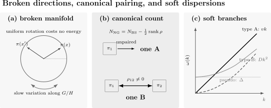
A slowly varying field moves along the broken-symmetry manifold rather than radially away from it. An unpaired broken direction gives one type-A mode, while two directions paired by a nonzero commutator density give one type-B mode. With ordinary leading derivatives, type-A modes are linear, type-B modes are quadratic, and weak explicit breaking lifts a would-be Goldstone mode to a nonzero gap.

Type A and Type B Versus Type I and Type II

The older Nielsen–Chadha classification labels modes by their low-momentum dispersion:

• type I for an odd leading power of $k$;
• type II for an even leading power of $k$.

The modern A/B classification labels the canonical structure:

• type A for an unpaired broken direction;
• type B for a canonically paired pair of broken directions.

In ordinary rotationally invariant local systems,

$$\text{type A} \longleftrightarrow \omega\sim k,$$

and

$$\text{type B} \longleftrightarrow \omega\sim k^2$$

are the generic outcomes. The classifications should not be identified without qualifications because accidental zeros or unusual derivative structures can alter the leading dispersion.

Neutral Superfluid Phonon

Symmetry and count

A neutral superfluid breaks global particle-number phase symmetry:

$$U(1) \longrightarrow \{1\}.$$

There is one broken generator,

$$Q = N,$$

and a one-dimensional antisymmetric commutator matrix is necessarily zero. Therefore

$$N_{\mathrm A} = 1, \qquad N_{\mathrm B} = 0.$$

The Goldstone field is the slowly varying condensate phase $\theta(\mathbf x,t)$.

Density is conjugate to phase

Let $\delta n$ be a density fluctuation. A minimal hydrodynamic Lagrangian is

$$\begin{aligned} \mathcal L ={}& \hbar\delta n\, \partial_t\theta - \frac{(\delta n)^2}{ 2\kappa_n } \\ &- \frac{\Upsilon}{2} \left( \boldsymbol\nabla\theta \right)^2, \end{aligned}$$

where

$$\kappa_n = \frac{\partial n}{\partial\mu}$$

is the number compressibility and $\Upsilon$ is the phase stiffness in this normalization.

The algebraic equation for density gives

$$\delta n = \kappa_n\hbar \partial_t\theta.$$

Eliminating $\delta n$ yields

$$\mathcal L_{\mathrm{eff}} = \frac{ \kappa_n\hbar^2 }{2} \left( \partial_t\theta \right)^2 - \frac{\Upsilon}{2} \left( \boldsymbol\nabla\theta \right)^2.$$

Hence

$$\omega(\mathbf k) = c_s k, \qquad c_s = \sqrt{ \frac{\Upsilon}{ \kappa_n\hbar^2 } }.$$

The density and phase oscillate together. Calling the mode “a phase wave” should not hide its measurable density response.

Bogoliubov benchmark

For a dilute repulsive Bose gas, microscopic Bogoliubov theory gives

$$E_k = \sqrt{ \epsilon_k \left( \epsilon_k+2gn_0 \right) },$$

where

$$\epsilon_k = \frac{\hbar^2k^2}{2m}.$$

At low momentum,

$$E_k \simeq \hbar c_s k.$$

Bogoliubov Theory owns that diagonalization and its stability conditions. Weakly Interacting Bose Gas Preview owns the dilute-gas scales and crossover to particle-like excitations.

The ideal Bose gas is a singular benchmark: it has macroscopic occupation but zero interaction stiffness, infinite compressibility in the condensed grand-canonical idealization, and quadratic bare-particle dispersion. A robust interacting superfluid phonon should not be inferred from condensation alone.

Ferromagnetic Magnon

An isotropic ferromagnet selects a magnetization direction, for example $z$:

$$SO(3) \longrightarrow SO(2).$$

The broken generators are $S^x$ and $S^y$. Their commutator is

$$\left[ S^x,S^y \right] = i\hbar S^z.$$

In a magnetized state,

$$m_z = \lim_{V\to\infty} \frac{\langle S^z\rangle}{V} \neq 0.$$

Therefore

$$\rho_{xy} = m_z,$$

and the broken-sector matrix has rank two. The count is

$$N_{\mathrm{BS}} = 2, \qquad N_{\mathrm B} = 1, \qquad N_{\mathrm A} = 0.$$

The two transverse tilts are canonically conjugate components of one magnon mode. Its long-wavelength dispersion is generically

$$\omega_{\mathrm{FM}}(\mathbf k) = Dk^2 + O(k^4).$$

For the nearest-neighbor Heisenberg ferromagnetic chain, the exact one-magnon result indeed approaches $k^2$. The Heisenberg Model owns the exchange-sign convention and exact lattice formula.

The $k=0$ lowering operator moves within the maximal-spin ground multiplet. The dispersing $k\neq0$ spin wave is the spatially varying Goldstone excitation. Magnons derives its Holstein–Primakoff quantization and contrasts it with the squeezed, two-sublattice antiferromagnetic construction.

Antiferromagnetic Magnons

A collinear antiferromagnet also has

$$SO(3) \longrightarrow SO(2),$$

so it breaks two generators. The crucial difference is that the selected Néel state has zero uniform spin density:

$$\lim_{V\to\infty} \frac{\langle\mathbf S_{\mathrm{tot}}\rangle}{V} = \mathbf0.$$

Consequently,

$$\operatorname{rank}\rho = 0,$$

and

$$N_{\mathrm A} = 2.$$

Let $\mathbf n$ be the unit Néel vector. Its leading effective Lagrangian is

$$\begin{aligned} \mathcal L_{\mathrm{AF}} = \frac{ \chi_\perp\hbar^2 }{2} \left( \partial_t\mathbf n \right)^2 \\ & - \frac{\rho_s}{2} \left( \boldsymbol\nabla\mathbf n \right)^2, \\ & \mathbf n^2 = 1. \end{aligned}$$

There are two transverse polarizations, both generically linear:

$$\omega_{\mathrm{AF}}(\mathbf q) \simeq c_{\mathrm{AF}} \lvert\mathbf q\rvert.$$

Depending on Brillouin-zone and sublattice conventions, these may be described as two polarizations of a degenerate branch or as branches associated with symmetry-related soft wavevectors.

The symmetry argument assumes an ordered antiferromagnetic thermodynamic phase. The spin-$1/2$ Heisenberg chain has no Néel long-range order in its ground state; its gapless spinon continuum is not a Goldstone magnon branch. Agreement on a linear low-energy scale does not establish the same quasiparticle content.

Acoustic Phonons in a Crystal

Broken translations

An isolated continuum crystal spontaneously breaks continuous translations to a discrete lattice. A displacement field

$$\mathbf u(\mathbf x,t)$$

labels slow local shifts of the ordered density pattern. A uniform displacement costs no bulk energy, so the elastic energy depends on strain:

$$u_{ij} = \frac12 \left( \partial_i u_j + \partial_j u_i \right).$$

The harmonic elastic Lagrangian is

$$\mathcal L_{\mathrm{el}} = \frac{\rho_m}{2} \dot u_i\dot u_i - \frac12 C_{ijkl} u_{ij}u_{kl}.$$

In an isotropic three-dimensional solid,

$$\begin{aligned} \omega_{\mathrm L} &= c_{\mathrm L}k, & c_{\mathrm L}^2 &= \frac{\lambda+2\mu}{\rho_m}, \\ \omega_{\mathrm T} &= c_{\mathrm T}k, & c_{\mathrm T}^2 &= \frac{\mu}{\rho_m}. \end{aligned}$$

There is one longitudinal and two transverse acoustic branches. In $d$ dimensions, an ordinary crystal has $d$ displacement components and hence $d$ acoustic phonon polarizations under the usual assumptions.

Why broken rotations add no ordinary branches

A crystal also breaks continuous rotations, yet it does not acquire an independent Goldstone field for every broken rotation. A slowly varying local rotation is already contained in spatial derivatives of $\mathbf u$. The local actions of broken translations and rotations are therefore redundant.

This is a spacetime-symmetry phenomenon. The internal formula based only on $\operatorname{rank}\rho$ must not be applied blindly.

What is not an acoustic Goldstone phonon

Optical phonons involve relative motion inside a unit cell and generally remain gapped at $k=0$. A crystal placed on a rigid substrate has continuous translation explicitly broken and can acquire a pinning gap. An electronic density wave on an imposed lattice may break only a discrete translation symmetry and does not automatically have a Goldstone mode.

An incommensurate density wave can possess an approximate sliding phase called a phason. Lattice commensurability, disorder, or Coulomb effects can pin or modify it. The exact symmetry of the physical Hamiltonian decides whether the phason is an exact Goldstone mode or a pseudo-Goldstone mode.

Three Kinds of Sound

Similar linear dispersions can have different origins:

Mode called “sound”	Infrared origin	Broken symmetry required?
normal-fluid first sound	hydrodynamic mass, momentum, and energy conservation	no
neutral-superfluid phonon	broken global $U(1)$ mixed with density	yes
crystal acoustic phonon	broken continuous translations	yes in a self-organized continuum crystal

A normal fluid preserves translations and particle-number phase symmetry, yet it supports hydrodynamic sound. Conservation laws and local equilibrium can produce a gapless collective mode without spontaneous symmetry breaking.

Conversely, a Goldstone mode can mix strongly with conserved densities. Classifying its origin requires the symmetry, state, and operator content, not only a plot of $\omega$ versus $k$.

Finite Systems

Momentum quantization

In a periodic box,

$$k_{\min} \sim \frac{2\pi}{L}.$$

For a generic type-A branch,

$$\hbar\omega_{\min}^{\mathrm A} \propto L^{-1},$$

whereas a generic type-B branch gives

$$\hbar\omega_{\min}^{\mathrm B} \propto L^{-2}.$$

Boundary conditions, aspect ratio, ordering wavevector, and anisotropic velocities must be held under control when fitting these powers.

Goldstone branch versus Anderson tower

The Anderson tower describes the nearly uniform quantum rotor of the entire order parameter. In a conventional antiferromagnet,

$$\Delta_{\mathrm{tower}} \sim L^{-d}.$$

The type-A spin wave instead has

$$\Delta_{\mathrm{wave}} \sim L^{-1}.$$

They are parametrically distinct for $d>1$. The tower consists of symmetry representations at momenta determined by the ordered state; the Goldstone branch consists of spatially varying excitations at nonzero wavevector.

The ferromagnet is exceptional: it can have an exactly degenerate maximal-spin multiplet at finite size and a type-B branch with $L^{-2}$ dispersion. Not every continuous broken phase exhibits the same rotor spectrum.

The zero mode

At exactly $\mathbf k=\mathbf0$, a uniform symmetry rotation may move within a degenerate ground-state manifold or become the finite-size rotor coordinate. It should not be double counted as an additional propagating quantum on top of the small nonzero-momentum branch.

Response and Spectral Signatures

Retarded response

For an operator $O_{\mathbf k}$ that overlaps with the broken direction,

$$\begin{aligned} \chi_{OO}^{R}(\mathbf k,\omega) = - \frac{i}{\hbar} \int_0^\infty dt\, e^{i(\omega+i0^+)t} \\ \times \left\langle \left[ O_{\mathbf k}(t), O_{-\mathbf k}(0) \right] \right\rangle . \end{aligned}$$

A stable Goldstone mode appears as a pole approaching zero frequency with momentum. In a scattering spectrum one may write schematically

$$\begin{aligned} S_O(\mathbf k,\omega) ={}& Z_O(\mathbf k) \delta\left( \omega-\omega_{\mathbf k} \right) \\ &+ S_O^{\mathrm{cont}}(\mathbf k,\omega). \end{aligned}$$

Interactions, finite temperature, disorder, and instrumental resolution broaden the line. A mode can also decay into other gapless excitations, so Goldstone status does not guarantee an infinitely sharp peak at every momentum.

Operator overlap

The residue

$$Z_O(\mathbf k)$$

depends on the probe. A transverse spin operator sees a magnon that a scalar density probe may miss. Neutron polarization, Bragg coupling, Raman tensor, and crystal form factors select different channels.

Failure to see a peak in one operator does not disprove the mode if symmetry forces that matrix element to vanish. Conversely, one soft peak does not establish Goldstone origin without the broken-symmetry evidence.

Representative probes

• neutron scattering measures spin-wave and magnon spectral weight;
• Brillouin, Raman, neutron, and inelastic x-ray scattering resolve phonons in different momentum and symmetry windows;
• Bragg spectroscopy probes density and spin modes in quantum gases;
• microwave and resonance experiments probe magnetic gaps and anisotropies;
• numerical analytic continuation and real-time evolution estimate dynamic correlators with resolution-dependent uncertainty.

Structure Factors owns normalization, detailed balance, and sum rules. Spectral Functions owns poles, continua, widths, and experimental convolution.

A Reliable Identification Workflow

Identify the exact symmetry

Write the symmetry group of the Hamiltonian, including fields, anisotropies, spin–orbit coupling, substrates, long-range terms, and boundary conditions. Separate exact, approximate, and emergent symmetries.

Establish spontaneous breaking

Use source-selected order, long-range correlations, structure-factor scaling, or another controlled thermodynamic diagnostic. A low-energy mode alone does not prove that the symmetry is broken.

Find the unbroken subgroup

Determine

$$G \longrightarrow H$$

and count the broken generators. Include all internal components and avoid counting gauge redundancies.

Evaluate the commutator matrix

For internal symmetries, compute

$$\rho_{ab} = - \frac{i}{\hbar V} \langle[Q_a,Q_b]\rangle$$

in the selected thermodynamic state. Use its rank to predict type-A and type-B counts.

Treat spacetime symmetries separately

Check whether broken transformations act redundantly on local fields. For crystals, displacements already encode local rotations.

Resolve momentum and quantum numbers

Track the correct soft wavevector, symmetry representation, polarization, and operator channel. A staggered mode can be missed by inspecting only $\mathbf k=\mathbf0$.

Scale energy and residue

Fit both

$$\omega_{\mathbf q}$$

and the spectral residue across system sizes and momenta. Compare linear, quadratic, gapped, and crossover forms with uncertainties.

Perturb the symmetry deliberately

Add a small symmetry-preserving perturbation and check robustness. Add a controlled explicit-breaking field and test whether the predicted pseudo-Goldstone gap appears.

Pseudo-Goldstone Modes

If an approximate continuous symmetry is weakly broken explicitly, the effective Lagrangian can acquire a restoring term:

$$\begin{aligned} \small \mathcal L_{\mathrm{pG}} = \frac{\chi\hbar^2}{2} \left( \partial_t\pi \right)^2 - \frac{\mathcal K}{2} \left( \boldsymbol\nabla\pi \right)^2 \\ & - \frac{ \chi\hbar^2\Delta^2 }{2} \pi^2. \end{aligned}$$

The dispersion becomes

$$\omega^2(\mathbf k) = \Delta^2 + v^2k^2.$$

The small gap $\Delta$ measures explicit breaking in the low-energy theory. Examples include:

• magnetic anisotropy or an applied field gapping a spin wave;
• a substrate pinning a translational phonon;
• commensurability or disorder pinning a sliding phase;
• weak microscopic terms breaking an emergent continuous symmetry.

Not every small gap is pseudo-Goldstone. The claim requires an identifiable larger symmetry recovered as the explicit-breaking parameter is removed.

Gauge Fields and Long-Range Forces

Gauge redundancy is not a broken global symmetry

A local gauge transformation is a redundancy, not an operation relating distinct physical states. Its “broken generators” must not be inserted into the global counting rule.

In a charged condensate coupled to a dynamical electromagnetic field, the phase mode and gauge field reorganize. In three dimensions, long-range Coulomb interactions produce a nonzero plasma frequency in the longitudinal sector. This Anderson–Higgs physics does not contradict the neutral global-symmetry result because the degrees of freedom and assumptions have changed.

Charged versus neutral limit

Turning off the gauge coupling or screening the long-range interaction can recover a neutral sound-like phase mode. The order of limits

$$k\to0, \qquad e\to0, \qquad \omega\to0$$

can matter. A statement about one limit should not be silently transferred to another.

Other long-range interactions

Dipolar forces, unscreened Coulomb interactions, and power-law couplings can change dispersion relations and the locality assumptions used in standard proofs. The symmetry pattern remains useful, but the short-range counting and derivative expansion require rechecking.

Spacetime-Symmetry Caveats

The internal counting rule assumes independent conserved internal charges in a translation-invariant setting. Broken spacetime symmetries require more care because:

• charge densities contain explicit coordinates;
• different broken transformations can generate the same local deformation;
• translations may themselves be broken;
• momentum and angular-momentum currents obey relations;
• background fields and boundaries can explicitly remove the symmetry.

Crystals are the canonical example: broken translations generate the displacement field, while broken rotations do not add independent ordinary branches. Superfluids similarly do not acquire an extra mode merely because a chosen rest frame fails to display Galilean boosts.

Temperature, Dimension, and Damping

The premise can fail

For short-range systems at nonzero temperature, continuous internal symmetry breaking is forbidden in sufficiently low dimensions under the Mermin–Wagner–Hohenberg assumptions. If there is no broken thermodynamic phase, the corresponding Goldstone theorem premise is absent.

Two-dimensional Berezinskii–Kosterlitz–Thouless phases have algebraic order and a sound-like phase mode, but no nonzero local condensate order parameter in the strict thermodynamic limit. Their infrared description should not be compressed into an ordinary three-dimensional broken-symmetry slogan.

Finite-temperature modes

At nonzero temperature, Goldstone variables couple to entropy, momentum, and other hydrodynamic densities. Modes can mix, split into first and second sound, or acquire damping. The static count of broken directions does not by itself determine every finite-temperature pole.

Superfluidity in Condensed Matter applies that finite-temperature mode splitting to neutral-material two-fluid and sound evidence; this page retains the symmetry and counting theory.

Open and driven systems

Dissipation can make frequencies complex and produce diffusive Goldstone modes. The equilibrium Hermitian counting rule is not automatically a theorem for Lindblad, active, Floquet, or driven steady states. State the dynamical framework before importing type-A/type-B conclusions.

Goldstone Modes Versus Other Gapless Excitations

Gapless structure	Goldstone mode?	Reason
ferromagnetic quadratic magnon	yes	broken spin rotations with nonzero commutator density
antiferromagnetic transverse magnon	yes in an ordered phase	broken spin rotations with zero commutator density
acoustic phonon of a self-organized crystal	yes, with spacetime caveats	broken translations
normal-fluid first sound	not by itself	hydrodynamic conservation laws
photon in vacuum	no	gauge field excitation, not a broken-global-symmetry mode
particle–hole continuum near a Fermi surface	no	kinematic gaplessness of an extended momentum-space manifold
soft mode exactly at a quantum critical point	not necessarily	criticality can occur without an ordered phase on either side
topological boundary mode	no in general	topology and anomaly constraints, not ordinary symmetry breaking
Ising domain wall	no	broken symmetry is discrete

Origins can mix. In a superfluid, the Goldstone phase couples to conserved density. In a supersolid, superfluid and elastic sectors can hybridize. Classification should identify the symmetry constraint and the dynamical mixture.

QFT Continuation

The many-body counting rule is one part of a broader field-theoretic story. From Symmetry Breaking to Goldstone Theorem develops the route through conserved currents, broken charges, spectral weight, and massless poles.

Continue to QFT.org when relativistic effective actions, Ward identities, renormalization, dynamical gauge fields, anomalies, or full quantum field theory become the central objects. Lorentz invariance restores stronger constraints: for ordinary broken internal symmetries, the charge-commutator density vanishes in the vacuum and each broken generator gives a linearly dispersing mode.

Common Mistakes

Counting broken generators as modes

In a nonrelativistic system, first compute $\operatorname{rank}\rho$. A ferromagnet is the standard counterexample to naive equality.

Defining type A as linear and type B as quadratic

Those dispersions are generic outcomes, not the definitions. A/B classifies canonical pairing of broken directions.

Calling every gapless excitation Goldstone

Hydrodynamic sound, photons, Fermi-surface continua, critical modes, and topological boundary states can be gapless for different reasons.

Applying the theorem to discrete symmetry breaking

Separated Ising-like branches do not provide a continuous flat direction. Domain walls are not Goldstone modes.

Ignoring the selected thermodynamic state

A finite symmetric ground state can hide the order. The theorem concerns the broken thermodynamic phase and its long-wavelength excitations.

Double counting the Anderson tower

The uniform rotor and the nonzero-momentum Goldstone branch are distinct finite-size structures.

Using only the dispersion exponent

A quadratic band minimum is not automatically type B, and a linear continuum edge is not automatically type A. Establish symmetry, order, quantum numbers, and spectral weight.

Counting broken rotations in a crystal independently

Spacetime symmetry actions can be redundant. The displacement field already contains local rotational deformations.

Treating optical phonons as mandatory Goldstone modes

Relative motion inside a unit cell is generally gapped and not forced by broken translations.

Ignoring explicit pinning

Anisotropy, fields, substrates, disorder, and commensurability can create pseudo-Goldstone gaps.

Treating gauge redundancy as a physical global symmetry

Charged condensates require gauge-invariant observables and electromagnetic dynamics. The neutral theorem cannot be copied unchanged.

Exercises

Exercise 1: Ferromagnet and antiferromagnet counting

Both a collinear isotropic ferromagnet and a collinear isotropic antiferromagnet break

$$SO(3) \longrightarrow SO(2).$$

Use

$$\left[ S^x,S^y \right] = i\hbar S^z$$

to count type-A and type-B modes in each case.

Solution

There are two broken generators in both systems:

$$N_{\mathrm{BS}} = 2.$$

In a ferromagnet selected along $z$,

$$\frac{\langle S^z\rangle}{V} = m_z \neq 0.$$

Hence the broken-sector commutator matrix is

$$\rho = \begin{pmatrix} 0&m_z \\ -m_z&0 \end{pmatrix},$$

which has rank two. Therefore

$$N_{\mathrm B} = 1, \qquad N_{\mathrm A} = 0.$$

The two transverse tilts form one type-B magnon.

In a collinear antiferromagnet, the staggered moment is nonzero but the uniform spin density vanishes:

$$\frac{\langle S^z\rangle}{V} = 0.$$

Thus $\rho=0$ and

$$N_{\mathrm A} = 2, \qquad N_{\mathrm B} = 0.$$

The two transverse Néel-vector fluctuations are type-A modes.

Exercise 2: Type-A dispersion

Starting from

$$\mathcal L = \frac{\chi\hbar^2}{2} \dot\pi^2 - \frac{\mathcal K}{2} \left( \boldsymbol\nabla\pi \right)^2,$$

derive the dispersion and the lowest finite-size energy in a periodic box of length $L$.

Solution

The Euler–Lagrange equation is

$$\chi\hbar^2 \partial_t^2\pi - \mathcal K\nabla^2\pi = 0.$$

For a plane wave,

$$- \chi\hbar^2\omega^2 + \mathcal K k^2 = 0.$$

Therefore

$$\omega = \sqrt{ \frac{\mathcal K}{ \chi\hbar^2 } } k = vk.$$

The smallest nonzero periodic momentum is

$$k_{\min} = \frac{2\pi}{L},$$

so

$$\hbar\omega_{\min} = \frac{2\pi\hbar v}{L} \propto L^{-1}.$$

Exercise 3: One mode from two type-B fields

For

$$\begin{aligned} \mathcal L ={}& \frac{\hbar s}{2} \left( \pi_1\dot\pi_2 - \pi_2\dot\pi_1 \right) \\ &- \frac{\mathcal K}{2} \left[ (\boldsymbol\nabla\pi_1)^2 + (\boldsymbol\nabla\pi_2)^2 \right], \end{aligned}$$

derive the dispersion and explain why there is one positive-frequency mode rather than two.

Solution

The equations are

$$\begin{aligned} \hbar s\,\dot\pi_1 &= \mathcal K\nabla^2\pi_2, \\ \hbar s\,\dot\pi_2 &= - \mathcal K\nabla^2\pi_1. \end{aligned}$$

Define

$$\psi = \pi_1+i\pi_2.$$

Up to the orientation convention for $s$, the two real equations combine into a first-order Schrödinger-type equation. Taking another time derivative gives

$$\omega^2 = \left( \frac{\mathcal K}{ \hbar s } \right)^2 k^4.$$

The positive-energy branch is

$$\omega = \frac{\mathcal K}{ \hbar\lvert s\rvert } k^2.$$

Because the Lagrangian is first order in time, $\pi_1$ and $\pi_2$ are a coordinate–momentum pair. They describe one oscillator per momentum, not two independent oscillators.

Exercise 4: Tower and wave scaling

In a $d$-dimensional antiferromagnet, suppose tower levels scale as $L^{-d}$ and type-A magnons scale as $L^{-1}$. For which $d$ are the two scales parametrically distinct? Why is equality of exponents in $d=1$ not evidence for Néel order?

Solution

For $d>1$,

$$L^{-d} \ll L^{-1}$$

at large $L$, so tower states collapse parametrically faster than the first nonzero-momentum magnon.

For $d=1$, both powers are $L^{-1}$. Exponents alone cannot distinguish the structures. One must inspect symmetry representations, momenta, matrix elements, and long-range-order scaling.

Moreover, the spin-$1/2$ Heisenberg antiferromagnetic chain does not have Néel long-range order. Its low-energy conformal tower and spinon excitations arise from a critical phase, not from an Anderson tower plus Goldstone magnons.

Exercise 5: Longitudinal and transverse phonons

For an isotropic elastic medium with mass density $\rho_m$ and Lamé coefficients $\lambda,\mu$, show that a plane-wave displacement separates into one longitudinal and $d-1$ transverse polarizations with

$$c_{\mathrm L}^2 = \frac{\lambda+2\mu}{\rho_m}, \qquad c_{\mathrm T}^2 = \frac{\mu}{\rho_m}.$$

Solution

The isotropic elastic equation is

$$\rho_m\ddot{\mathbf u} = (\lambda+\mu) \boldsymbol\nabla \left( \boldsymbol\nabla\cdot\mathbf u \right) + \mu\nabla^2\mathbf u.$$

For a longitudinal wave,

$$\mathbf u \parallel \mathbf k,$$

both terms contribute, giving

$$\omega_{\mathrm L}^2 = \frac{\lambda+2\mu}{\rho_m} k^2.$$

For a transverse wave,

$$\mathbf k\cdot\mathbf u = 0,$$

the divergence term vanishes:

$$\omega_{\mathrm T}^2 = \frac{\mu}{\rho_m} k^2.$$

There is one longitudinal direction and a $(d-1)$-dimensional transverse subspace.

Exercise 6: Pseudo-Goldstone gap

Add

$$- \frac{\chi\hbar^2\Delta^2}{2} \pi^2$$

to the type-A Lagrangian. Derive the dispersion and identify the limits that recover an exact Goldstone mode.

Solution

The equation becomes

$$\chi\hbar^2 \left( \partial_t^2+\Delta^2 \right) \pi - \mathcal K\nabla^2\pi = 0.$$

For a plane wave,

$$\omega^2 = \Delta^2 + \frac{\mathcal K}{ \chi\hbar^2 } k^2.$$

At $k=0$, the excitation gap is $\hbar\Delta$. The exact Goldstone limit is recovered by removing the explicit-breaking parameter so that

$$\Delta \to 0$$

after the thermodynamic phase has been defined.

Exercise 7: Classifying gapless excitations

Classify each excitation as Goldstone, non-Goldstone, or assumption dependent:

1. a photon in vacuum;
2. first sound in a normal fluid;
3. a quadratic magnon in an isotropic ferromagnet;
4. an Ising domain wall;
5. an acoustic phonon in an isolated continuum crystal;
6. a soft order-parameter mode exactly at a quantum critical point.

Solution

1. A photon is not a Goldstone mode of broken global symmetry; it is a gauge-field excitation.
2. Normal-fluid first sound is hydrodynamic and follows from conservation laws and local equilibrium, not necessarily broken symmetry.
3. The ferromagnetic magnon is a type-B Goldstone mode.
4. An Ising domain wall belongs to broken discrete symmetry and is not a Goldstone mode.
5. An acoustic phonon is a spacetime Goldstone mode of broken translations, with rotational redundancy caveats.
6. A critical soft mode is not automatically Goldstone. At the critical point the ordered phase may not yet exist, and critical scaling rather than motion along a broken manifold controls the gaplessness.

Exercise 8: Charged condensate

A neutral superfluid has a linear phase mode. Explain why replacing its particles by charged particles and coupling them to dynamical electromagnetism can produce a plasma gap without contradicting Goldstone reasoning.

Solution

The neutral derivation assumes a physical global $U(1)$ phase degree of freedom with short-range interactions. Dynamical electromagnetism introduces a gauge redundancy, a gauge field, and a long-range Coulomb interaction.

The phase fluctuation and longitudinal electromagnetic field are no longer independent neutral variables. They hybridize, and in three dimensions the longitudinal collective mode approaches a nonzero plasma frequency:

$$\omega(k\to0) \longrightarrow \omega_p > 0.$$

The assumptions and physical degrees of freedom have changed, so the neutral theorem has not been violated. Gauge-invariant electromagnetic response must be analyzed in the charged system.

Key Takeaways

• Broken continuous global symmetry forces low-energy collective dynamics under stated assumptions.
• In nonrelativistic systems, the number of Goldstone modes can be smaller than the number of broken generators.
• The commutator-density matrix gives $N_{\mathrm{NG}}=N_{\mathrm{BS}}-\frac12\operatorname{rank}\rho$ for broken internal symmetries.
• Type-A modes come from unpaired broken directions; type-B modes come from canonically paired directions.
• Linear type-A and quadratic type-B dispersions are generic, not definitional.
• A neutral superfluid has one type-A phonon.
• A ferromagnet has one type-B magnon, while a collinear antiferromagnet has two type-A transverse modes.
• Acoustic phonons are spacetime Goldstone modes of broken translations; broken rotations do not add independent ordinary branches.
• The finite-size Anderson tower and the nonzero-momentum Goldstone branch are distinct.
• Pseudo-Goldstone gaps require identifiable weak explicit breaking.
• Hydrodynamic, critical, gauge, Fermi-surface, and topological gaplessness have different origins.
• Gauge coupling, long-range interactions, dimensionality, temperature, and dissipation can modify the naive picture.

Further Reading

• Spontaneous Symmetry Breaking – selected phases, finite-size rotors, and Anderson towers.
• Goldstone Modes Preview – compact symmetry-first orientation.
• From Symmetry Breaking to Goldstone Theorem – currents, charges, spectral weight, and the QFT bridge.
• Phonons as Many-Body Excitations – dynamical matrices, lattice-mode quantization, acoustic and optical branches, and phonon operators.
• Bogoliubov Theory – microscopic neutral-superfluid phonons.
• Heisenberg Model – exact ferromagnetic magnons and antiferromagnetic spin-wave benchmarks.
• Structure Factors – experimental and numerical spectra.
• QFT.org – relativistic field theory, Ward identities, gauge fields, and effective actions.

References

1. Y. Nambu, “Quasi-Particles and Gauge Invariance in the Theory of Superconductivity”, Physical Review 117, 648–663 (1960).
2. J. Goldstone, “Field Theories with Superconductor Solutions”, Il Nuovo Cimento 19, 154–164 (1961).
3. J. Goldstone, A. Salam, and S. Weinberg, “Broken Symmetries”, Physical Review 127, 965–970 (1962).
4. P. W. Anderson, “Plasmons, Gauge Invariance, and Mass”, Physical Review 130, 439–442 (1963).
5. H. B. Nielsen and S. Chadha, “On How to Count Goldstone Bosons”, Nuclear Physics B 105, 445–453 (1976).
6. H. Leutwyler, “Nonrelativistic Effective Lagrangians”, Physical Review D 49, 3033–3043 (1994).
7. H. Watanabe and T. Brauner, “Number of Nambu–Goldstone Bosons and Its Relation to Charge Densities”, Physical Review D 84, 125013 (2011).
8. H. Watanabe and H. Murayama, “Unified Description of Nambu–Goldstone Bosons without Lorentz Invariance”, Physical Review Letters 108, 251602 (2012).
9. Y. Hidaka, “Counting Rule for Nambu–Goldstone Modes in Nonrelativistic Systems”, Physical Review Letters 110, 091601 (2013).
10. H. Watanabe and H. Murayama, “Redundancies in Nambu–Goldstone Bosons”, Physical Review Letters 110, 181601 (2013).
11. H. Watanabe and H. Murayama, “Effective Lagrangian for Nonrelativistic Systems”, Physical Review X 4, 031057 (2014).
12. H. Watanabe, “Counting Rules of Nambu–Goldstone Modes”, Annual Review of Condensed Matter Physics 11, 169–187 (2020).
13. T. Holstein and H. Primakoff, “Field Dependence of the Intrinsic Domain Magnetization of a Ferromagnet”, Physical Review 58, 1098–1113 (1940).
14. P. C. Hohenberg, “Existence of Long-Range Order in One and Two Dimensions”, Physical Review 158, 383–386 (1967).
15. N. D. Mermin and H. Wagner, “Absence of Ferromagnetism or Antiferromagnetism in One- or Two-Dimensional Isotropic Heisenberg Models”, Physical Review Letters 17, 1133–1136 (1966).