Long-Range Order

Long-range order is the persistence of a specified correlation pattern across arbitrarily large separations in a many-body or thermodynamic limit.

For a local ordering operator $O_j$ and an ordering wavevector $\mathbf Q$, the characteristic statement is

$$\lim_{|\mathbf r|\to\infty} e^{-i\mathbf Q\cdot\mathbf r} \left\langle O_0^\dagger O_{\mathbf r} \right\rangle = m_{\mathbf Q}^2 > 0.$$

This equation is compact, but it is not self-interpreting. One must specify:

• the operator, its components, and its normalization;
• the state or ensemble;
• the spatial dimension, temperature, and interaction range;
• the order in which volume and distance limits are taken;
• whether the correlator is full or connected;
• whether $\mathbf Q$ is fixed, optimized, or symmetry averaged;
• whether the claimed limit is pointwise or spatially averaged.

The same order can usually be diagnosed without selecting a nonzero one-point function. If

$$M_{\mathbf Q} = \sum_{j\in\Lambda} e^{-i\mathbf Q\cdot\mathbf r_j}O_j$$

is the extensive ordering mode in a region containing $N_\Lambda$ sites, then conventional long-range order is equivalently signaled, under standard homogeneity assumptions, by

$$\liminf_{\Lambda\uparrow\mathbb Z^d} \frac{ \left\langle M_{\mathbf Q}^\dagger M_{\mathbf Q} \right\rangle }{ N_\Lambda^2 } > 0.$$

This squared-order criterion remains useful when every finite-volume state respects the symmetry and therefore has $\langle M_{\mathbf Q}\rangle=0$.

Canonical Scope

This page is the canonical home for conventional diagonal long-range order in many-body quantum mechanics. It owns:

• pointwise and volume-averaged correlation criteria;
• the relation among real-space plateaus, squared order parameters, and extensive structure-factor peaks;
• the roles of full and connected correlations in selected phases and symmetric states;
• short-range, algebraic, and true long-range scaling at finite size;
• uniform, staggered, spiral, density-wave, and crystalline examples;
• finite-size, boundary, domain, commensurability, and resolution caveats;
• practical numerical and experimental tests for a long-range-order claim.

Neighboring pages retain separate ownership:

• Order Parameters defines microscopic ordering operators, extensive modes, intensive normalizations, and conjugate sources.
• Equal-Time Correlations owns operator ordering and static two-point conventions.
• Connected Correlation Functions develops cumulant subtraction, cluster decomposition, correlation lengths, and pure-phase versus mixture analysis.
• Structure Factors owns Fourier conventions, dynamic and static structure factors, scattering normalization, and sum rules.
• Spontaneous Symmetry Breaking owns Hamiltonian versus state symmetry, source selection, finite-volume cat states, and tower spectra.
• Susceptibilities owns response functions and their frequency and momentum limits.
• Bose–Einstein Condensation owns the ideal-gas mechanism and bosonic benchmark. Off-Diagonal Long-Range Order treats one- and two-body density-matrix criteria systematically.
• Crystalline Symmetry Preview owns the symmetry groups of crystals; the present page only previews correlation and Bragg diagnostics.
• Model pages retain exact phase diagrams, spectra, and model-specific amplitudes.

The word conventional matters. Topological order, string order, many-body localization, and some forms of quantum order are not characterized by a nonzero asymptote of a local two-point function.

Setup and Conventions

Let $\Lambda_L$ be a sequence of $d$-dimensional regions with linear scale $L$, volume $V_L$, and $N_L$ lattice sites. For a regular lattice at fixed density,

$$N_L \propto L^d.$$

Choose a bounded local operator $O_j$. It may be:

• a spin component $S_j^a$;
• a density deviation $n_j-\bar n$;
• a sublattice or orbital polarization;
• a local composite such as a quadrupole;
• one component of a vector or tensor order parameter.

For a candidate ordering wavevector $\mathbf Q$, define

$$\begin{aligned} M_{\mathbf Q,L} &= \sum_{j\in\Lambda_L} e^{-i\mathbf Q\cdot\mathbf r_j}O_j, \\ m_{\mathbf Q,L} &= \frac{M_{\mathbf Q,L}}{N_L}. \end{aligned}$$

The phase convention is arbitrary provided it is used consistently. With this convention,

$$\begin{aligned} \left\langle m_{\mathbf Q,L}^\dagger m_{\mathbf Q,L} \right\rangle &= \frac{1}{N_L^2} \sum_{i,j\in\Lambda_L} e^{i\mathbf Q\cdot(\mathbf r_i-\mathbf r_j)} \\ &\qquad\times \left\langle O_i^\dagger O_j \right\rangle. \end{aligned}$$

For Hermitian $O_j$, this quantity is real and nonnegative. For a non-Hermitian operator, the dagger order is essential.

Translation-invariant form

If the state and geometry are translation invariant, define

$$C(\mathbf r) = \left\langle O_0^\dagger O_{\mathbf r} \right\rangle$$

and remove the candidate oscillation:

$$C_{\mathbf Q}(\mathbf r) = e^{-i\mathbf Q\cdot\mathbf r} C(\mathbf r).$$

Then

$$\left\langle m_{\mathbf Q,L}^\dagger m_{\mathbf Q,L} \right\rangle = \frac{1}{N_L} \sum_{\mathbf r} w_L(\mathbf r) C_{\mathbf Q}(\mathbf r),$$

where $w_L(\mathbf r)$ is the fraction of ordered pairs at displacement $\mathbf r$ that remain inside $\Lambda_L$. For periodic boundaries, $w_L=1$ on the finite torus. For open boundaries, it tends to one at fixed $\mathbf r$ as $L\to\infty$.

This identity is the bridge between a long-distance correlation plateau and a macroscopic squared order parameter.

Vector and tensor operators

For an $n$-component Hermitian operator $\mathbf O_j$, a symmetry-neutral estimator is

$$\mathcal M_{\mathbf Q,L}^2 = \frac{1}{N_L^2} \sum_{a=1}^{n} \left\langle M_{\mathbf Q,L}^{a\dagger} M_{\mathbf Q,L}^{a} \right\rangle.$$

It can remain nonzero in a finite state that averages uniformly over all orientations. Component-resolved normalizations must be stated: in an isotropic mixture, a single component often carries only $1/n$ of the rotationally invariant weight.

Continuum systems

For a continuum operator density $O(\mathbf x)$ in a region $\Lambda$, replace sums by integrals:

$$M_{\mathbf Q,\Lambda} = \int_\Lambda d^d x\, e^{-i\mathbf Q\cdot\mathbf x} O(\mathbf x).$$

Contact terms and ultraviolet distributions affect short separations and integrated sum rules, but not a nonzero large-distance plateau after the operator has been properly defined.

Three Long-Range-Order Diagnostics

Three formulations recur across theory, numerics, and experiment. They are closely related but not logically identical without assumptions.

Pointwise correlation limit

The strongest elementary criterion is

$$\lim_{|\mathbf r|\to\infty} C_{\mathbf Q}(\mathbf r) = m_{\mathbf Q}^2 > 0.$$

This says that the phase-corrected correlation approaches the same nonzero number along every sufficiently regular direction. It is appropriate for a homogeneous phase with a single commensurate ordering pattern.

The limit may fail to exist even though order is present. Common causes include:

• several symmetry-related ordering wavevectors;
• incommensurate order with an imprecisely chosen $\mathbf Q$;
• anisotropic directional limits;
• quasiperiodic or multi-$\mathbf Q$ patterns;
• boundaries, interfaces, or macroscopic domains;
• disorder realizations that are not translation invariant.

For these cases, an averaged criterion is safer.

Volume-averaged criterion

One robust definition is

$$\liminf_{L\to\infty} \left\langle m_{\mathbf Q,L}^\dagger m_{\mathbf Q,L} \right\rangle = m_{\mathbf Q,\mathrm{av}}^2 > 0.$$

Equivalently,

$$\liminf_{L\to\infty} \frac{ \left\langle M_{\mathbf Q,L}^\dagger M_{\mathbf Q,L} \right\rangle }{ N_L^2 } > 0.$$

The liminf allows finite-size oscillations and subsequences. It also makes the order of limits explicit: first define the state on each growing region, then study the macroscopic observable.

This criterion is weaker than a pointwise plateau. A positive spatial average guarantees macroscopic coherent weight in the chosen mode, but by itself does not prove that every long-distance direction converges to one constant. Additional homogeneity, ergodicity, or regularity assumptions connect the two.

Structure-factor criterion

With the static convention

$$S_O(\mathbf q;L) = \frac{1}{N_L} \left\langle M_{\mathbf q,L}^\dagger M_{\mathbf q,L} \right\rangle,$$

the squared-order estimator is exactly

$$\left\langle m_{\mathbf Q,L}^\dagger m_{\mathbf Q,L} \right\rangle = \frac{S_O(\mathbf Q;L)}{N_L}.$$

Thus true long-range order produces an extensive peak:

$$S_O(\mathbf Q;L) = N_L m_{\mathbf Q}^2 +o(N_L).$$

The peak height alone is convention dependent. Some authors omit the factor $1/N_L$ from $S_O$, in which case the ordered peak scales as $N_L^2$. A reliable statement always reports both the Fourier convention and the asymptotic scaling.

In an infinite translation-invariant description, the persistent correlation contributes a Bragg delta function:

$$S_O(\mathbf q) \supset (2\pi)^d m_{\mathbf Q}^2 \delta^{(d)}(\mathbf q-\mathbf Q),$$

with reciprocal-lattice copies and convention-dependent volume factors understood. On a finite sample the delta function appears as a resolution-limited peak whose height grows and width narrows.

When the Diagnostics Agree

Suppose:

1. the density and sample shape approach fixed limits;
2. boundary contributions are subextensive;
3. the phase-corrected correlator is bounded;
4. $C_{\mathbf Q}(\mathbf r)\to m_{\mathbf Q}^2$ at large separation.

Then a vanishing fraction of the double sum comes from pairs at short separation. The remaining $O(N_L^2)$ distant pairs each contribute approximately $m_{\mathbf Q}^2$, so

$$\frac{ \left\langle M_{\mathbf Q,L}^\dagger M_{\mathbf Q,L} \right\rangle }{ N_L^2 } \longrightarrow m_{\mathbf Q}^2.$$

This is a many-dimensional Cesàro-average statement: convergence of the pointwise correlator implies convergence of its macroscopic spatial average.

The converse needs more care. A nonzero average can coexist with:

• different limits in different directions;
• a finite set of macroscopically occupied wavevectors;
• phase separation or a macroscopic interface;
• sample-to-sample random signs;
• a sequence of geometries commensurate with only selected patterns.

In practice, establish the averaged scaling and then inspect real-space directionality, peak locations, boundary dependence, and order-parameter distributions.

Full Correlations, Connected Correlations, and Clustering

Long-range order is normally identified from a full correlation function. Connected subtraction answers a different question: whether fluctuations remain correlated after one-point expectation values have been removed.

Define

$$\begin{aligned} G(i,j) &= \left\langle O_i^\dagger O_j \right\rangle, \\ G_c(i,j) &= G(i,j) - \left\langle O_i^\dagger\right\rangle \left\langle O_j\right\rangle. \end{aligned}$$

Selected clustering phase

Suppose an extremal ordered phase has

$$\left\langle O_j\right\rangle_\alpha = m_\alpha e^{i\mathbf Q\cdot\mathbf r_j}.$$

Cluster decomposition gives

$$\begin{aligned} e^{-i\mathbf Q\cdot\mathbf r} \left\langle O_0^\dagger O_{\mathbf r} \right\rangle_\alpha &\longrightarrow |m_\alpha|^2, \\ e^{-i\mathbf Q\cdot\mathbf r} \left\langle O_0^\dagger O_{\mathbf r} \right\rangle_{c,\alpha} &\longrightarrow 0. \end{aligned}$$

The phase has long-range order even though its connected correlator decays. The plateau is the disconnected product of the selected one-point values.

Symmetric mixture

Now average equally over two branches with order parameters $\pm m$. The mixture has

$$\left\langle O_j\right\rangle_{\mathrm{mix}} = 0,$$

but

$$e^{-i\mathbf Q\cdot\mathbf r} \left\langle O_0^\dagger O_{\mathbf r} \right\rangle_{\mathrm{mix}} \longrightarrow m^2.$$

Because the one-point function vanishes, the connected correlator has the same plateau. The residual correlation records uncertainty in one global phase label; it does not show that a local fluctuation propagates without decay.

For an isotropic mixture of an $n$-component vector order parameter with fixed magnitude $m$, rotational averaging gives

$$\lim_{|\mathbf r|\to\infty} \left\langle O_0^a O_{\mathbf r}^b \right\rangle_{\mathrm{mix}} = \frac{m^2}{n} \delta_{ab}.$$

Summing over components restores the full rotationally invariant weight $m^2$.

Finite symmetric pure states

A finite-volume cat state can be a pure vector and still have

$$\left\langle M_{\mathbf Q,L}\right\rangle = 0, \qquad \left\langle M_{\mathbf Q,L}^\dagger M_{\mathbf Q,L} \right\rangle \sim N_L^2.$$

For fixed local observables, its thermodynamic limit may become indistinguishable from a classical mixture of ordered branches. The Spontaneous Symmetry Breaking page develops the source-selected limits and finite-size spectra behind this behavior. The Connected Correlation Functions page owns the general cluster-property analysis.

Long-Range Order and Spontaneous Symmetry Breaking

The concepts are tightly related but should not be identified without qualification.

What long-range order establishes

For a local operator transforming nontrivially under a global symmetry, macroscopic squared order shows that the finite or symmetric state contains coherent weight in an ordering channel. Under locality and commutator assumptions, such order can support the construction of low-lying states and symmetry-breaking thermodynamic phases.

Schematically,

$$\begin{gathered} \text{local long-range order} \\ + \ \text{appropriate thermodynamic limit} \\ \Longrightarrow \text{ symmetry-breaking states}. \end{gathered}$$

Rigorous versions require hypotheses. They are not consequences of one large finite-size data point.

What it does not establish alone

A long-range-order estimator does not by itself prove:

• that the Hamiltonian has the relevant symmetry;
• that the order is spontaneous rather than explicitly pinned;
• that the limiting state is extremal;
• that a continuous family of phases exists;
• that there are Goldstone modes;
• that the order survives at nonzero temperature;
• that a local Landau order parameter completely classifies the phase.

Conversely, an explicitly symmetry-breaking field can give $\langle O\rangle\ne0$ without a phase transition or spontaneous order. The field must be removed after the thermodynamic limit to test spontaneous selection.

Finite-Size Scaling Regimes

No finite sample contains an infinite separation. The diagnosis therefore rests on how correlations and peaks scale along a controlled sequence of sizes.

Assume that the phase-corrected correlator behaves over a broad range as

$$C_{\mathbf Q}(r) \sim \frac{A}{r^p}$$

in $d$ dimensions. Summing over a ball of radius $L$ gives

$$S_O(\mathbf Q;L) \sim \int_a^L dr\, r^{d-1-p}.$$

The leading regimes are:

• True long-range order

  $$\begin{aligned} C_{\mathbf Q}(r) &\longrightarrow m^2>0, \\ S_O(\mathbf Q;L) &\sim m^2L^d, \\ \frac{S_O(\mathbf Q;L)}{N_L} &\longrightarrow m^2. \end{aligned}$$

• Algebraic order with $0<p<d$

  $$\begin{aligned} C_{\mathbf Q}(r) &\sim r^{-p}, \\ S_O(\mathbf Q;L) &\sim L^{d-p}, \\ \frac{S_O(\mathbf Q;L)}{N_L} &\sim L^{-p}. \end{aligned}$$

• Marginal algebraic decay with $p=d$

  $$\begin{aligned} S_O(\mathbf Q;L) &\sim \log L, \\ \frac{S_O(\mathbf Q;L)}{N_L} &\sim L^{-d}\log L. \end{aligned}$$

• Integrable algebraic decay with $p>d$

  $$\begin{aligned} S_O(\mathbf Q;L) &= O(1), \\ \frac{S_O(\mathbf Q;L)}{N_L} &= O(L^{-d}). \end{aligned}$$

• Exponential decay at fixed $\xi$

  $$\begin{aligned} S_O(\mathbf Q;L) &= O(\xi^d), \\ \frac{S_O(\mathbf Q;L)}{N_L} &= O \left( \frac{\xi^d}{L^d} \right). \end{aligned}$$

Algebraic correlations can generate a rapidly growing peak while the normalized quantity $S_O(\mathbf Q;L)/N_L$ still vanishes. A growing peak is therefore not, by itself, proof of true long-range order.

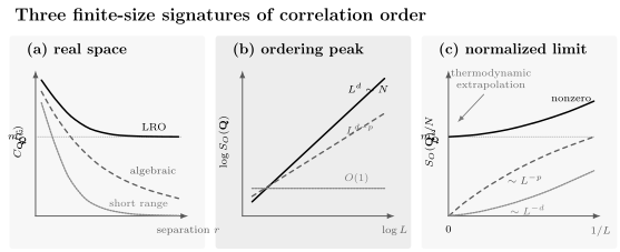
The same three regimes viewed through the phase-corrected correlator, peak-height scaling, and the normalized estimator $S_O(\mathbf Q;L)/N_L$. True long-range order approaches a nonzero plateau; algebraic order gives a subextensive peak; short-range correlations saturate at fixed correlation length.

True long-range order

In an ordered phase,

$$C_{\mathbf Q}(r) = m_{\mathbf Q}^2 + \delta C_{\mathbf Q}(r), \qquad \delta C_{\mathbf Q}(r)\to0.$$

Therefore,

$$S_O(\mathbf Q;L) = N_Lm_{\mathbf Q}^2 + S_{\mathrm{fluc}}(\mathbf Q;L).$$

The correction may be constant, algebraic, logarithmic, or geometry dependent. Goldstone fluctuations often make finite-size convergence much slower than a naive $1/N_L$ extrapolation.

Algebraic or quasi-long-range order

If $C_{\mathbf Q}(r)$ decays as a power law to zero, the state has algebraic order or quasi-long-range order, not true long-range order in the strict plateau sense.

For $0<p<d$,

$$S_O(\mathbf Q;L) \propto L^{d-p},$$

which is divergent but subextensive. The exponent may vary continuously along a phase, as in Berezinskii–Kosterlitz–Thouless physics, or take a critical value only at a transition.

Short-range order

If the connected correlations decay exponentially,

$$C_{\mathbf Q}(r) \sim A r^{-\sigma}e^{-r/\xi},$$

then $S_O(\mathbf Q;L)$ approaches a finite limit once $L\gg\xi$. The normalized peak therefore vanishes as $1/N_L$.

The full correlator in a selected ordered phase is an exception to the phrase “decays exponentially”: its connected correction may decay exponentially while the full correlator approaches $m_{\mathbf Q}^2$.

Critical crossover

When $L\lesssim\xi$, a disordered system can look scale-free or nearly ordered. Reliable extrapolation needs sizes on both sides of the crossover and, near a critical point, a scaling form such as

$$S_O(\mathbf Q;L,g) = L^{d-p_*} \mathcal F \left( (g-g_c)L^{1/\nu} \right),$$

where $p_*$ is the equal-time critical correlation exponent in the convention being used. It is safer to define $p_*$ through the measured correlator than to import a classical formula without accounting for the dynamical exponent and equal-time slice.

The canonical transition analysis belongs to Quantum Phase Transitions.

Correlation Length Inside an Ordered Phase

An ordered phase can have both infinite-range order and a finite correlation length. There is no contradiction.

Write

$$C_{\mathbf Q}(r) = m_{\mathbf Q}^2 + C_{\mathbf Q,c}(r).$$

The constant is the ordered background. A correlation length characterizes the decay of $C_{\mathbf Q,c}$, not the full correlator:

$$C_{\mathbf Q,c}(r) \sim r^{-\sigma}e^{-r/\xi}.$$

For a continuous broken symmetry, Goldstone modes can instead make the connected correction algebraic, so no finite exponential correlation length describes that channel. Other massive channels may still have finite correlation lengths.

Magnetic Long-Range Order

Magnetic systems provide the cleanest lattice examples because the local operators and ordering wavevectors are explicit.

Ferromagnetic order

For spin operators $\mathbf S_j$, define the total magnetization

$$\mathbf M = \sum_j \mathbf S_j.$$

Uniform ferromagnetic order has $\mathbf Q=\mathbf0$ and

$$\lim_{|\mathbf r|\to\infty} \left\langle \mathbf S_0\cdot\mathbf S_{\mathbf r} \right\rangle = m_{\mathrm F}^2 > 0,$$

or equivalently

$$\lim_{N\to\infty} \frac{\langle\mathbf M^2\rangle}{N^2} = m_{\mathrm F}^2.$$

In a selected phase, $\langle\mathbf S_j\rangle$ points along one direction. In a rotationally invariant mixture, the vector one-point function vanishes but $\langle\mathbf M^2\rangle/N^2$ remains finite.

Néel order

On a bipartite lattice, let $\eta_j=+1$ on sublattice $A$ and $-1$ on sublattice $B$. The staggered magnetization is

$$\mathbf M_{\mathrm s} = \sum_j \eta_j\mathbf S_j.$$

For a hypercubic nearest-neighbor antiferromagnet, this corresponds to

$$\mathbf Q = (\pi,\ldots,\pi)$$

in units of the inverse lattice spacing. A rotationally invariant finite-size estimator is

$$m_{\mathrm s}^2(L) = \frac{1}{N_L^2} \sum_{i,j} \eta_i\eta_j \left\langle \mathbf S_i\cdot\mathbf S_j \right\rangle.$$

If $m_{\mathrm s}^2(L)\to m_{\mathrm s}^2>0$, the sequence has Néel long-range order even if

$$\left\langle\mathbf M_{\mathrm s}\right\rangle = 0$$

at every finite size.

For an $SU(2)$-invariant state,

$$\left\langle M_{\mathrm s}^aM_{\mathrm s}^b \right\rangle = \frac{\delta_{ab}}{3} \left\langle \mathbf M_{\mathrm s}^2 \right\rangle.$$

Comparing a one-component estimator with a dot-product estimator therefore requires a factor of three.

The three-dimensional spin-$1/2$ cubic antiferromagnet has rigorous Néel-order results. For the two-dimensional square-lattice spin-$1/2$ model, zero-temperature Néel order is supported by extensive analytical and numerical evidence, while the short-range isotropic model has no nonzero-temperature continuous magnetic long-range order. The Heisenberg Model page owns the model-specific evidence and conventions.

Spiral and multi-wavevector order

A spiral may have

$$\left\langle S_j^x+iS_j^y \right\rangle = m e^{i\mathbf Q\cdot\mathbf r_j}.$$

Then $M_{\mathbf Q}$ is the natural complex ordering mode. A real spin pattern generally produces paired peaks at $\pm\mathbf Q$. A multi-$\mathbf Q$ state requires a set of modes and their relative phases; one peak does not reconstruct the full texture.

Finite clusters can frustrate an incommensurate pitch because allowed momenta are discrete. Twisted boundaries, elongated sequences, or interpolation of the peak location may be needed before extrapolating its height.

Discrete Ising order

For the transverse-field Ising convention used in the model page, $\sigma_j^z$ is the ordering operator and the field points along $x$:

$$M_z = \sum_j\sigma_j^z.$$

An exact finite parity eigenstate can satisfy

$$\langle M_z\rangle = 0, \qquad \frac{\langle M_z^2\rangle}{N^2} > 0$$

throughout the ordered regime as $N\to\infty$. Equivalently,

$$\left\langle \sigma_0^z\sigma_r^z \right\rangle \longrightarrow m_z^2.$$

This is the standard example in which correlations reveal order before a branch is explicitly selected. Exact amplitudes and the critical point belong to the Transverse-Field Ising Model.

Density-Wave Order

Let

$$\delta n_j = n_j-\bar n.$$

A charge-density wave at $\mathbf Q$ has

$$\rho_{\mathbf Q} = \frac{1}{N} \sum_j e^{-i\mathbf Q\cdot\mathbf r_j} \delta n_j$$

and long-range order when

$$\lim_{N\to\infty} \left\langle \rho_{\mathbf Q}^\dagger\rho_{\mathbf Q} \right\rangle > 0.$$

For a period-two pattern in one dimension, $\mathbf Q=\pi$ and

$$\lim_{r\to\infty} (-1)^r \left\langle \delta n_0\delta n_r \right\rangle = \rho_\pi^2.$$

The two translated patterns are symmetry-related. A finite translation eigenstate may have $\langle\rho_\pi\rangle=0$ while retaining the correlation plateau.

The half-filled nearest-neighbor spinless-fermion chain provides a zero-temperature discrete density-wave example. Its gapless regime instead has algebraic $2k_{\mathrm F}$ correlations, demonstrating why a growing peak must be divided by system size and extrapolated. Model details belong to Spinless Fermion Chains.

Spin-density waves, orbital-density waves, and bond-density waves use the same logic with different local or bond operators. The operator must match the symmetry pattern: density correlations cannot diagnose pure bond order if the density remains uniform.

For the materials-facing distinction among finite-width correlations, static order, reconstructed bands, and mechanism claims, see Charge and Spin Density Waves.

Crystalline Order Preview

A crystal breaks continuous translations to a discrete space group. In a selected classical-looking configuration, the mean density is periodic:

$$\left\langle n(\mathbf x)\right\rangle = \bar n + \sum_{\mathbf G\ne\mathbf0} n_{\mathbf G} e^{i\mathbf G\cdot\mathbf x},$$

where $\mathbf G$ runs over reciprocal-lattice vectors.

An exact finite translation eigenstate can have uniform one-point density. Define instead

$$\rho_{\mathbf q} = \sum_{a=1}^{N} e^{-i\mathbf q\cdot\mathbf r_a}.$$

Crystalline long-range order produces Bragg scaling

$$\frac{ \left\langle \rho_{\mathbf G}^\dagger\rho_{\mathbf G} \right\rangle }{ N^2 } \longrightarrow B_{\mathbf G} > 0$$

for reciprocal vectors $\mathbf G$. Equivalently, the density-density correlation retains periodic components at arbitrarily large separation.

The coefficient $B_{\mathbf G}$ includes zero-point and thermal displacement fluctuations. In a harmonic description, a Debye–Waller factor suppresses the Bragg weight:

$$B_{\mathbf G} \propto \left| \left\langle e^{-i\mathbf G\cdot\mathbf u} \right\rangle \right|^2,$$

where $\mathbf u$ is the displacement field. Whether this factor remains nonzero depends on dimension, temperature, interactions, and the type of positional order.

At nonzero temperature, ordinary three-dimensional crystals can have true translational long-range order. Two-dimensional crystals with short-range interactions typically have only algebraic positional order, so their Bragg peaks are singular but not extensive in the strict plateau sense. Orientational order can behave differently. These statements require the hypotheses of the low-dimensional fluctuation analysis and should not be reduced to a slogan.

The Crystalline Symmetry Preview develops the group-theoretic language. Detailed elasticity, defects, and melting belong to later statistical-mechanics treatments.

Bragg Peaks and What Scattering Measures

Elastic neutron, X-ray, and atom scattering provide momentum-space access to order. A perfectly static ordered component contributes at zero energy transfer:

$$S_O(\mathbf q,\omega) \supset 2\pi S_{O,\mathrm{el}}(\mathbf q) \delta(\omega).$$

At an ordering wavevector,

$$S_{O,\mathrm{el}}(\mathbf Q) \propto N m_{\mathbf Q}^2$$

in the normalized static convention used on this page. Real instruments replace delta functions by resolution functions in momentum and frequency.

A sharp observed peak is not automatically a thermodynamic Bragg peak. One must test:

• how its height and integrated weight depend on sample volume;
• whether its width is instrument limited or intrinsic;
• whether the signal is elastic, quasielastic, or inelastic;
• whether finite domains set the width;
• whether several orientations or twins contribute;
• whether form factors and polarization project out components;
• whether the background and disconnected forward peak were removed consistently.

The canonical relation among dynamic scattering, equal-time integration, and normalization is developed in Structure Factors.

Finite-Size Caveats

Finite systems can both hide genuine order and imitate it. A credible analysis keeps the following effects explicit.

The order of distance and volume limits

On a finite periodic lattice, the largest independent separation is only of order $L/2$. The intended thermodynamic statement is

$$\lim_{|\mathbf r|\to\infty} \lim_{L\to\infty} C_{\mathbf Q,L}(\mathbf r),$$

with $\mathbf r$ held well inside the sample while the volume is enlarged first. Setting $r=L/2$ defines a useful finite-size estimator, but its extrapolation is not literally the same iterated limit without scaling control.

A practical window is

$$a \ll r \ll L,$$

where $a$ is a microscopic scale. Near criticality, one also needs $r$ large compared with irrelevant crossover lengths.

Symmetry-preserving finite states

Periodic exact diagonalization, tensor-network calculations with enforced symmetry, and unbiased Monte Carlo often produce

$$\left\langle m_{\mathbf Q,L} \right\rangle = 0.$$

This is expected and does not imply absence of order. Use

$$\left\langle m_{\mathbf Q,L}^\dagger m_{\mathbf Q,L} \right\rangle,$$

the large-distance full correlator, or the order-parameter probability distribution.

Conversely, an open-boundary calculation or unconstrained variational state may select a branch at finite size. A nonzero $\langle m_{\mathbf Q,L}\rangle$ then demonstrates pinning or variational selection, not by itself a nonzero thermodynamic limit.

Boundary pinning

Open boundaries can induce an order profile even in a disordered phase:

$$\left\langle O_j\right\rangle_{\mathrm{open}} \sim e^{-d_j/\xi},$$

where $d_j$ is the distance from the boundary. Measure in a central window and vary both $L$ and the window size. In an ordered phase, boundary pinning can be useful for selecting an orientation, but the central amplitude must stabilize as the boundary recedes.

Aspect ratio and shape

Long thin samples can cross over to effectively lower-dimensional behavior. Fix aspect ratios when possible and compare several shapes. Goldstone modes, domain walls, and incommensurate patterns can have unusually strong shape dependence.

The thermodynamic limit is a sequence, not merely a large site count. Thermodynamic Limit develops admissible sequences and boundary corrections.

Commensurability

If $\mathbf Q$ is incompatible with the finite torus, the true peak lies between allowed momenta. The measured value at the nearest grid point can underestimate order and oscillate with $L$.

Useful responses include:

• choosing commensurate subsequences;
• tracking the maximum over nearby momenta;
• using twisted boundary conditions;
• fitting the peak shape rather than one momentum bin;
• reporting how the inferred $\mathbf Q_L$ approaches its limit.

Optimizing over too broad a momentum set introduces its own finite-size bias. The search rule must be fixed before extrapolation.

Multiple domains

A macroscopic sample may contain symmetry-related domains. The spatial average of the one-point order can vanish while diffraction still shows Bragg peaks. Domain size broadens the peaks and changes real-space correlations at separations beyond a typical domain.

If the number of domains grows with volume and their orientations are uncorrelated, the global squared mode can become subextensive even though each domain is locally ordered. The thermodynamic conclusion depends on whether the domain structure is an equilibrium pure phase, a mixture, a metastable preparation, or disorder pinned.

Phase coexistence

At a first-order transition, a finite system can contain two phases separated by an interface. A large value of $\langle m^2\rangle$ may then reflect coexistence rather than a homogeneous ordered phase. Histograms, Binder ratios, interface free energies, and boundary-condition dependence help distinguish these cases. Finite-Temperature Phase Transitions develops the two-phase finite-size picture and the inverse-volume rounding scale.

Conserved quantities

Fixing a global charge can create a weak compensating tail in connected correlations. For example, if

$$\sum_j\delta n_j = 0$$

exactly, then the spatial sum of the connected density correlator is constrained. A negative $O(1/N)$ background can coexist with otherwise short-range correlations. Such a tail is not long-range order because its amplitude vanishes with volume.

Statistical and truncation error

Squared modes can be differences of large contributions or be dominated by long-distance samples with poor signal-to-noise. Autocorrelation, symmetry-sector tunneling, tensor-network bond dimension, Monte Carlo population bias, and finite-time averaging can all distort the apparent plateau.

The uncertainty must be propagated through the extrapolation, not attached only to each raw size.

Windowed and Inhomogeneous Estimators

For open, trapped, or disordered systems, define a weighted mode

$$M_{\mathbf Q}[w] = \sum_j w_j e^{-i\mathbf Q\cdot\mathbf r_j} O_j.$$

A normalized estimator is

$$m_{\mathbf Q}^2[w] = \frac{ \left\langle M_{\mathbf Q}[w]^\dagger M_{\mathbf Q}[w] \right\rangle }{ \left(\sum_j w_j\right)^2 }.$$

The weights may select a central region, match a known density profile, or suppress a noisy edge. They also broaden momentum resolution. Results should be checked against a family of windows whose bulk fraction has a controlled limit.

In a trap, a single global Fourier mode can average over several local phases. Real-space maps, connected subtraction with the local profile, and local-density reasoning may be more informative than one global peak.

Low-Dimensional Constraints

Long-range-order claims must state dimension, temperature, symmetry, and interaction range.

Continuous internal symmetries at nonzero temperature

For broad classes of one- and two-dimensional systems with sufficiently short-range interactions, thermal infrared fluctuations forbid conventional long-range order that would break a continuous internal symmetry. The Mermin–Wagner theorem establishes this for isotropic Heisenberg-type models under its assumptions, and Hohenberg’s argument treats the related continuum condensate problem.

This does not exclude:

• discrete symmetry breaking in two dimensions;
• zero-temperature order in two-dimensional quantum systems;
• explicit anisotropy that reduces the symmetry;
• sufficiently long-range interactions;
• finite samples with a large correlation length;
• algebraic order and Berezinskii–Kosterlitz–Thouless behavior.

One-dimensional discrete order

The one-dimensional short-range classical Ising chain has no nonzero-temperature long-range order because finite-energy domain walls occur at nonzero density. This mechanism is not the Mermin–Wagner theorem.

At zero temperature, a one-dimensional quantum system can break a discrete symmetry. The ordered phase of the transverse-field Ising chain is the canonical example.

Positional order

Translations are continuous symmetries, and displacement fluctuations are especially infrared sensitive. For ordinary short-range systems at nonzero temperature:

• three-dimensional crystals can retain nonzero Bragg weights;
• two-dimensional crystals generally have algebraic translational order;
• one-dimensional positional correlations are still more strongly disrupted.

Substrate potentials, long-range forces, quenched pinning, and nonequilibrium preparation can change these conclusions.

Zero temperature is not obtained by slogan

Quantum ground-state fluctuations add an imaginary-time dimension to scaling, but the equal-time correlator still lives on a spatial slice. Whether order survives depends on the model, symmetry, dispersion, and dynamical exponent. There is no universal rule that simply replaces $d$ by $d+1$ in every long-range-order criterion.

Distinctions from Other Uses of “Long Range”

Long-range interactions

Long-range order concerns the asymptotic behavior of a state. Long-range interactions concern the spatial decay of Hamiltonian terms, for example

$$J(r) \sim \frac{1}{r^\alpha}.$$

A short-range Hamiltonian can have long-range order, and a long-range Hamiltonian can be disordered. Long-range interactions can alter critical exponents, locality bounds, and low-dimensional no-go results, but they do not change the basic definition.

Off-diagonal long-range order

Conventional density or spin order uses correlations diagonal in the relevant local observable basis. Condensation and superconducting pairing are more naturally defined through macroscopic eigenvalues of reduced density matrices.

For a number-conserving bosonic state, a one-body correlator may satisfy

$$\left\langle \psi^\dagger(\mathbf x) \psi(\mathbf y) \right\rangle \not\to 0$$

as $|\mathbf x-\mathbf y|\to\infty$. This is off-diagonal long-range order and has normalization, gauge, dimensional, and fragmentation subtleties beyond the present page. See Bose–Einstein Condensation for the canonical condensate criterion.

String and hidden order

A local two-point correlator can decay while a nonlocal string correlator approaches a constant. For example, define

$$\mathcal U_{ij} = \exp\left( i\pi\sum_{k=i+1}^{j-1}Q_k \right).$$

Then hidden order can appear as

$$\left\langle O_i\mathcal U_{ij}O_j \right\rangle \longrightarrow \text{constant}.$$

This is long-range order of a nonlocal operator, not conventional local long-range order. The operator support grows with separation, so cluster arguments for two fixed local observables do not apply unchanged.

Topological order

Topologically ordered phases can have exponentially decaying correlations for every local operator while retaining ground-state topology, long-range entanglement, and nonlocal loop diagnostics. The absence of a local correlation plateau therefore does not imply that a phase is trivial.

Spin-glass order

In a disordered magnet, the disorder-averaged two-point function may vanish even when frozen local moments persist. An Edwards–Anderson-type diagnostic squares or time-averages local correlations before disorder averaging. That is not the same as a coherent Bragg mode at one $\mathbf Q$.

Large susceptibility

A susceptibility measures response:

$$\chi_{\mathbf Q} = \frac{1}{N} \int_0^\beta d\tau\, \left\langle M_{\mathbf Q}(\tau) M_{\mathbf Q}^\dagger(0) \right\rangle_c.$$

It can be large near a transition while $S_O(\mathbf Q)/N$ still vanishes. Equal-time order, zero-frequency response, and adiabatic response involve different limits and should not be substituted for one another.

A Reliable Numerical Workflow

Choose the operator before fitting

State the microscopic operator, its components, form factor, and symmetry transformation. A failed dipolar correlator does not rule out quadrupolar, bond, or composite order.

Determine the ordering wavevector

Inspect the full momentum dependence on several sizes. Check symmetry-related peaks and commensurability. Do not choose $\mathbf Q$ solely from the largest noisy bin of the largest sample.

Preserve one normalization

Record

$$S_O(\mathbf q) = \frac{1}{N} \left\langle M_{\mathbf q}^\dagger M_{\mathbf q} \right\rangle$$

or the alternative convention once, and use it in every plot. The thermodynamic estimator is then $S_O(\mathbf Q)/N$ in this convention.

Compare real and momentum space

Plot $C_{\mathbf Q}(r)$ against both $r$ and $r/L$. Fit a plateau plus corrections, a power law, and an exponential only over windows where each ansatz is physically justified. Confirm that the real-space conclusion matches peak scaling.

Resolve symmetry and phase selection

Report whether the calculation enforces symmetry, uses a pinning field, or allows spontaneous variational selection. Compare full and connected correlators accordingly.

Scale shapes, boundaries, and errors

Use several $L$, preferably with fixed aspect ratio. Repeat selected sizes under different boundaries or windows. Include covariance and systematic fit-window uncertainty in the extrapolation.

Cross-check another observable

Depending on the problem, useful cross-checks include:

• an order-parameter histogram;
• a Binder cumulant or correlation ratio;
• a susceptibility;
• a low-energy tower or symmetry-sector splitting;
• a stiffness;
• a domain-wall free energy;
• an elastic scattering weight.

No one cross-check is universal. The goal is a mutually consistent phase fingerprint.

Experimental Interpretation

Experiments observe finite samples for finite times. Long-range order is inferred rather than literally measured at infinite separation.

Diffraction

Magnetic neutron diffraction and X-ray or atom diffraction identify symmetry-allowed Bragg positions, polarization channels, and volume scaling. Peak width estimates a lower bound on domain or correlation length only after instrumental resolution is deconvolved.

Real-space probes

Quantum-gas microscopes and imaging experiments can estimate $C(\mathbf r)$ directly over the field of view. Spatial inhomogeneity, parity projection, detection loss, and fixed-number constraints must be included in the estimator.

Local probes

Nuclear magnetic resonance, muon spin rotation, and local microscopy can detect a static internal field or local modulation. Such evidence is powerful for branch-selected order but does not alone map the full ordering wavevector or establish a thermodynamic scaling law.

Time resolution

Slowly fluctuating domains may appear static within an instrumental window. Separating elastic from quasielastic weight is essential when distinguishing genuine static order from slow dynamics.

Common Mistakes

• Inferring absence of order from $\langle M_{\mathbf Q}\rangle=0$ in a finite symmetry eigenstate.
• Calling any increasing structure-factor peak long-range order without checking whether it is extensive.
• Forgetting to divide $S_O(\mathbf Q)$ by $N$ in the convention used here.
• Fitting the full correlator in an ordered phase to an exponential without subtracting its plateau.
• Calling an algebraic decay to zero a nonzero long-range limit.
• Using a connected correlator plateau in a symmetric mixture as evidence for a propagating infinite-range fluctuation.
• Comparing one spin component with a rotationally invariant dot-product estimator without the component factor.
• Choosing an incommensurate $\mathbf Q$ from one finite momentum grid and holding the wrong value fixed.
• Treating boundary-induced order as a bulk limit without moving the boundary away.
• Ignoring domains, phase coexistence, aspect ratio, or order-parameter histograms.
• Applying Mermin–Wagner without stating temperature, dimension, symmetry, and interaction range.
• Confusing long-range order with long-range interactions.
• Using a local two-point criterion to rule out topological or string order.
• Treating a sharp finite-resolution peak as a delta function without size or resolution analysis.
• Claiming a universal finite-size correction such as $1/L$ without identifying the low-energy modes that produce it.

Exercises

Exercise 1: From a plateau to extensive peak scaling

On a periodic translation-invariant lattice with $N$ sites, suppose

$$C_{\mathbf Q}(\mathbf r) = m^2+f(\mathbf r),$$

where

$$\frac{1}{N} \sum_{\mathbf r} f(\mathbf r) \longrightarrow 0.$$

Show that

$$S_O(\mathbf Q) = Nm^2+o(N).$$

Solution

Translation invariance gives

$$S_O(\mathbf Q) = \sum_{\mathbf r} C_{\mathbf Q}(\mathbf r).$$

Therefore,

$$\begin{aligned} S_O(\mathbf Q) &= \sum_{\mathbf r} \left[ m^2+f(\mathbf r) \right] \\ &= Nm^2 + \sum_{\mathbf r}f(\mathbf r). \end{aligned}$$

The assumption says

$$\sum_{\mathbf r}f(\mathbf r) = o(N),$$

so

$$S_O(\mathbf Q) = Nm^2+o(N).$$

Dividing by $N$ recovers the squared-order estimator $m^2$.

Exercise 2: Algebraic correlations

Suppose a $d$-dimensional phase has

$$C_{\mathbf Q}(r) \sim A r^{-p}$$

with $0<p<d$. Derive the leading scaling of $S_O(\mathbf Q;L)$ and $S_O(\mathbf Q;L)/N_L$.

Solution

Approximating the lattice sum by a radial integral,

$$\begin{aligned} S_O(\mathbf Q;L) &\sim A\int_a^L dr\,r^{d-1-p} \\ &\sim \frac{A}{d-p} L^{d-p}. \end{aligned}$$

Since $N_L\propto L^d$,

$$\frac{S_O(\mathbf Q;L)}{N_L} \propto L^{-p} \longrightarrow 0.$$

The peak diverges, but it is subextensive. The state has algebraic rather than true long-range order.

Exercise 3: Selected phase and symmetric mixture

Two clustering phases satisfy

$$\langle O_j\rangle_\pm = \pm m$$

and

$$\langle O_iO_j\rangle_\pm \longrightarrow m^2.$$

Compute the long-distance full and connected correlators in either selected phase and in their equal mixture.

Solution

In either selected phase,

$$\langle O_iO_j\rangle_\pm \longrightarrow m^2,$$

while

$$\begin{aligned} \langle O_iO_j\rangle_{c,\pm} &= \langle O_iO_j\rangle_\pm - \langle O_i\rangle_\pm \langle O_j\rangle_\pm \\ &\longrightarrow m^2-m^2 = 0. \end{aligned}$$

In the equal mixture,

$$\langle O_j\rangle_{\mathrm{mix}} = \frac{m+(-m)}{2} = 0,$$

but linearity gives

$$\langle O_iO_j\rangle_{\mathrm{mix}} \longrightarrow m^2.$$

The connected correlator in the mixture therefore also tends to $m^2$. It records the unresolved global branch label and shows that the mixture does not cluster.

Exercise 4: Component normalization in a Néel state

An $SU(2)$-invariant finite state satisfies

$$\langle M_{\mathrm s}^aM_{\mathrm s}^b\rangle = A_L\delta_{ab}.$$

Express $A_L$ in terms of $\langle\mathbf M_{\mathrm s}^2\rangle$. If the dot-product estimator approaches $m_{\mathrm s}^2$, what does the single-$z$-component estimator approach?

Solution

Summing over $a=b=x,y,z$ gives

$$\left\langle \mathbf M_{\mathrm s}^2 \right\rangle = 3A_L.$$

Hence

$$A_L = \frac{1}{3} \left\langle \mathbf M_{\mathrm s}^2 \right\rangle.$$

If

$$\frac{ \left\langle \mathbf M_{\mathrm s}^2 \right\rangle }{N^2} \longrightarrow m_{\mathrm s}^2,$$

then

$$\frac{ \left\langle (M_{\mathrm s}^z)^2 \right\rangle }{N^2} \longrightarrow \frac{m_{\mathrm s}^2}{3}.$$

The factor is geometric, not evidence that one estimator detects weaker order.

Exercise 5: Fixed correlation length

In $d$ dimensions, assume

$$C_{\mathbf Q}(r) = A e^{-r/\xi}$$

with $\xi$ independent of $L$. Estimate the large-$L$ scaling of $S_O(\mathbf Q;L)$ and the squared-order estimator.

Solution

The infinite-volume spatial integral converges:

$$\begin{aligned} S_O(\mathbf Q;\infty) &\sim A\int_0^\infty dr\, r^{d-1}e^{-r/\xi} \\ &= A\Gamma(d)\xi^d \end{aligned}$$

up to angular and lattice factors. Thus the peak approaches $O(\xi^d)$ rather than growing with $N$. Consequently,

$$\frac{S_O(\mathbf Q;L)}{N_L} = O \left( \frac{\xi^d}{L^d} \right) \longrightarrow 0.$$

Large but fixed $\xi$ can imitate order on sizes $L\lesssim\xi$, which is why the asymptotic size regime matters.

Exercise 6: Translation averaging in a crystal

Let $|\Phi_{\mathbf a}\rangle$ denote a crystalline state translated by $\mathbf a$, with

$$\langle\Phi_{\mathbf a}|\rho_{\mathbf G}|\Phi_{\mathbf a}\rangle = N n_{\mathbf G} e^{-i\mathbf G\cdot\mathbf a}.$$

Form a uniform incoherent mixture over translations in one unit cell. Show that $\langle\rho_{\mathbf G}\rangle=0$ for $\mathbf G\ne\mathbf0$ while $\langle\rho_{\mathbf G}^\dagger\rho_{\mathbf G}\rangle/N^2$ remains $|n_{\mathbf G}|^2$ when branch fluctuations are subleading.

Solution

Translation averaging gives

$$\langle\rho_{\mathbf G}\rangle_{\mathrm{mix}} = Nn_{\mathbf G} \int_{\mathrm{cell}} \frac{d^d a}{V_{\mathrm{cell}}} e^{-i\mathbf G\cdot\mathbf a}.$$

For nonzero reciprocal vector $\mathbf G$, the phase averages to zero over translations modulo the lattice:

$$\langle\rho_{\mathbf G}\rangle_{\mathrm{mix}} = 0.$$

In each branch,

$$\left| \langle\rho_{\mathbf G}\rangle_{\mathbf a} \right|^2 = N^2|n_{\mathbf G}|^2.$$

The translation phase cancels in the modulus. If connected branch fluctuations are $o(N^2)$, linear averaging gives

$$\frac{ \langle \rho_{\mathbf G}^\dagger\rho_{\mathbf G} \rangle_{\mathrm{mix}} }{N^2} \longrightarrow |n_{\mathbf G}|^2.$$

Thus a translation-invariant state can retain crystalline Bragg order in a two-point diagnostic.

Exercise 7: A conserved-density tail

Suppose a periodic system has fixed total particle number, so

$$\sum_j\delta n_j = 0$$

in every state. Show that

$$\sum_j \left\langle \delta n_i\delta n_j \right\rangle = 0.$$

Explain why a uniform negative tail of amplitude $O(1/N)$ is not long-range order.

Solution

Multiply the operator constraint by $\delta n_i$ and take the expectation value:

$$\begin{aligned} 0 &= \left\langle \delta n_i \sum_j\delta n_j \right\rangle \\ &= \sum_j \left\langle \delta n_i\delta n_j \right\rangle. \end{aligned}$$

Positive short-distance correlations must therefore be balanced by negative weight elsewhere. On a finite homogeneous system, that compensation can appear as an approximately uniform background proportional to $-1/N$.

Long-range order requires a nonzero amplitude after the thermodynamic limit. Since $1/N\to0$, the constraint-induced tail vanishes and contributes at most $O(1)$ to the structure factor, not an extensive $O(N)$ peak.

Exercise 8: Classifying finite-size evidence

For each observation, state the strongest justified conclusion.

1. $S(\mathbf Q;L)\propto L^{d-0.3}$ over a controlled asymptotic range.
2. $S(\mathbf Q;L)/N_L\to0.12$ with stable aspect-ratio and boundary checks.
3. An open sample has nonzero central $\langle O\rangle$, but the central value decays as $e^{-L/(2\xi)}$.
4. A local correlator decays exponentially, while a nonlocal string correlator approaches a constant.

Solution

1. The peak is divergent but subextensive. The evidence supports algebraic order with exponent $p=0.3$, not a nonzero local correlation plateau.
2. In the stated normalization, the evidence supports conventional long-range order in the $\mathbf Q$ channel with squared amplitude $0.12$, subject to correct operator choice and error control.
3. The one-point value is boundary induced and vanishes as the boundary recedes. This evidence supports a finite correlation length, not bulk long-range order.
4. There is no conventional local long-range order in the tested operator, but there is long-range order of the specified nonlocal string operator. That distinction must be kept explicit.

Key Takeaways

• Long-range order is a property of an operator, state, pattern, and thermodynamic limit.
• A nonzero phase-corrected correlation plateau implies macroscopic squared order and an extensive structure-factor peak under standard homogeneity assumptions.
• With $S_O(\mathbf q)=\langle M_{\mathbf q}^\dagger M_{\mathbf q}\rangle/N$, the finite-size order estimator is $S_O(\mathbf Q)/N$.
• A finite symmetry eigenstate can have zero one-point order while its squared order remains macroscopic.
• In a selected clustering phase, the full correlator plateaus and the connected correlator decays; a symmetric mixture can retain the plateau in both.
• Algebraic order produces a divergent but subextensive peak and no nonzero plateau.
• Correlation lengths in ordered phases describe connected corrections, not the constant ordered background.
• Magnetic, density-wave, and crystalline order use the same correlation logic with different operators and wavevectors.
• Boundaries, commensurability, domains, conservation laws, and finite resolution can hide or imitate asymptotic order.
• Conventional local long-range order is distinct from long-range interactions, off-diagonal order, string order, spin-glass order, and topological order.

Further Reading

• Order Parameters – operator, component, source, and normalization dictionary.
• Spontaneous Symmetry Breaking – thermodynamic branch selection and finite-size spectra.
• Equal-Time Correlations – static correlator conventions.
• Connected Correlation Functions – cluster decomposition and correlation lengths.
• Structure Factors – Fourier and scattering conventions.
• Antiferromagnetism – an extensive finite-wavevector ordering peak, magnetic Bragg diffraction, and low-dimensional material constraints.
• Heisenberg Model – ferromagnetic and Néel examples.
• Transverse-Field Ising Model – discrete symmetry breaking in a finite parity eigenstate.
• Spinless Fermion Chains – algebraic and density-wave regimes.
• Low-Dimensional Quantum Gases – infrared fluctuation constraints.
• Crystalline Symmetry Preview – crystal symmetry and reciprocal lattices.

References

1. J. Fröhlich, B. Simon, and T. Spencer, “Infrared Bounds, Phase Transitions and Continuous Symmetry Breaking”, Communications in Mathematical Physics 50, 79–95 (1976).
2. F. J. Dyson, E. H. Lieb, and B. Simon, “Phase Transitions in Quantum Spin Systems with Isotropic and Nonisotropic Interactions”, Journal of Statistical Physics 18, 335–383 (1978).
3. T. Kennedy, E. H. Lieb, and B. S. Shastry, “Existence of Néel Order in Some Spin-1/2 Heisenberg Antiferromagnets”, Journal of Statistical Physics 53, 1019–1030 (1988).
4. T. Kennedy, E. H. Lieb, and B. S. Shastry, “The XY Model Has Long-Range Order for All Spins and All Dimensions Greater Than One”, Physical Review Letters 61, 2582–2584 (1988).
5. K. Kubo and T. Kishi, “Existence of Long-Range Order in the XXZ Model”, Physical Review Letters 61, 2585–2587 (1988).
6. P. Horsch and W. von der Linden, “Spin-Correlations and Low Lying Excited States of the Spin-1/2 Heisenberg Antiferromagnet on a Square Lattice”, Zeitschrift für Physik B Condensed Matter 72, 181–193 (1988).
7. K. J. Runge, “Quantum Monte Carlo Calculation of the Long-Range Order in the Heisenberg Antiferromagnet”, Physical Review B 45, 7229–7236 (1992).
8. T. Koma and H. Tasaki, “Symmetry Breaking and Finite-Size Effects in Quantum Many-Body Systems”, Journal of Statistical Physics 76, 745–803 (1994).
9. H. Tasaki, “Long-Range Order, ‘Tower’ of States, and Symmetry Breaking in Lattice Quantum Systems”, Journal of Statistical Physics 174, 735–761 (2019).
10. H. Tasaki, Physics and Mathematics of Quantum Many-Body Systems, Springer (2020).
11. N. D. Mermin and H. Wagner, “Absence of Ferromagnetism or Antiferromagnetism in One- or Two-Dimensional Isotropic Heisenberg Models”, Physical Review Letters 17, 1133–1136 (1966).
12. P. C. Hohenberg, “Existence of Long-Range Order in One and Two Dimensions”, Physical Review 158, 383–386 (1967).
13. N. D. Mermin, “Crystalline Order in Two Dimensions”, Physical Review 176, 250–254 (1968).
14. L. van Hove, “Correlations in Space and Time and Born Approximation Scattering in Systems of Interacting Particles”, Physical Review 95, 249–262 (1954).
15. B. Nachtergaele and R. Sims, “Lieb–Robinson Bounds and the Exponential Clustering Theorem”, Communications in Mathematical Physics 265, 119–130 (2006).
16. C. N. Yang, “Concept of Off-Diagonal Long-Range Order and the Quantum Phases of Liquid He and of Superconductors”, Reviews of Modern Physics 34, 694–704 (1962).