Low-Dimensional Quantum Gases

A low-dimensional quantum gas is a many-particle gas whose thermally and dynamically accessible motion is restricted to one or two spatial directions. The phrase includes genuinely one- or two-dimensional models and experimentally realized quasi-one-dimensional or quasi-two-dimensional gases in which strong confinement freezes the remaining directions.

Dimensionality is not a cosmetic change of coordinates. For particles with quadratic dispersion,

$$\epsilon_{\mathbf k} = \frac{\hbar^2k^2}{2m},$$

the density of one-particle states per active volume behaves as

$$\frac{D_d(\epsilon)}{V_d} \propto \epsilon^{d/2-1}.$$

It diverges at the band edge in one dimension, is constant in two dimensions, and vanishes as $\sqrt{\epsilon}$ in three dimensions. That single change reorganizes ideal-gas thermodynamics, the infrared capacity of a Bose gas, the geometry of a Fermi sea, and the importance of long-wavelength fluctuations.

Low dimension does not merely reduce the number of momentum components. It increases the relative weight of low-energy modes, where statistics, interactions, and collective fluctuations are hardest to ignore.

This page owns uniform one- and two-dimensional state counting, ideal Bose and Fermi consequences, the distinction between strict and effective dimensionality, and the fluctuation logic that points toward low-dimensional many-body physics. Bose–Einstein Condensation owns the full condensation criterion. Sommerfeld Expansion owns systematic low-temperature Fermi integrals. Lieb–Liniger Model Preview owns the exact finite-coupling contact gas, while Tonks–Girardeau Gas Preview owns the impenetrable Bose–Fermi map. This page previews the Berezinskii–Kosterlitz–Thouless transition; Superfluidity in Condensed Matter applies that logic to neutral films and their material evidence, while the Luttinger-liquid page owns its dedicated theory.

Ultracold Atoms owns the platform-level freeze-out, trap-calibration, and interaction-tuning checks used to establish that a laboratory gas realizes this regime.

What Counts as Low Dimensional?

Three different statements are often compressed into the same phrase.

1. A strictly $d$-dimensional model has configuration space $\mathbb R^d$, a $d$-dimensional measure, and interactions defined in that dimension.
2. A kinematically quasi-$d$-dimensional gas lives in three-dimensional space but occupies only the transverse ground mode over the energies being probed.
3. A geometrically anisotropic gas is merely much longer or wider in some directions. It need not be dynamically low dimensional if excited transverse modes are populated.

For example, a long cigar-shaped cloud is not automatically one dimensional. It becomes quasi-one-dimensional only when transverse excitations are energetically inaccessible and interactions do not strongly admix them.

If a transverse direction is harmonically confined with frequency $\omega_\perp$, adjacent transverse levels are separated by

$$\Delta_\perp = \hbar\omega_\perp.$$

A practical low-energy requirement is

$$E_{\mathrm{active}} \ll \hbar\omega_\perp,$$

where $E_{\mathrm{active}}$ must include every relevant scale: $k_{\mathrm B}T$, a Fermi energy, interaction energy per particle, collective-mode frequencies, drive bandwidths, and any chemical-potential offset measured from the transverse ground threshold.

The word effective matters. A sample can be one dimensional for equilibrium thermodynamics and three dimensional during a violent quench that excites transverse motion.

Uniform State Counting in d Dimensions

Consider a large periodic box with active $d$-dimensional volume $V_d$ and internal multiplicity $g$. One momentum state occupies volume $(2\pi)^d/V_d$ in $\mathbf k$-space. The number of states inside a sphere of radius $k$ is therefore

$$\mathcal N_d(k) = g\frac{V_d}{(2\pi)^d} \frac{S_{d-1}}{d}k^d,$$

where

$$S_{d-1} = \frac{2\pi^{d/2}}{\Gamma(d/2)}$$

is the area of the unit $(d-1)$-sphere.

For quadratic dispersion,

$$k = \frac{\sqrt{2m\epsilon}}{\hbar}.$$

The integrated density of states becomes

$$\frac{\mathcal N_d(\epsilon)}{V_d} = \frac{g}{\Gamma(d/2+1)} \left( \frac{m}{2\pi\hbar^2} \right)^{d/2} \epsilon^{d/2}.$$

Differentiating with respect to energy gives the density of states

$$\frac{D_d(\epsilon)}{V_d} = \frac{g}{\Gamma(d/2)} \left( \frac{m}{2\pi\hbar^2} \right)^{d/2} \epsilon^{d/2-1}.$$

Here $V_1=L$, $V_2=A$, and $V_3=V$. The units change with dimension: $D_1/L$ is a density per length per energy, while $D_2/A$ is a density per area per energy.

The one- and two-dimensional formulas

The explicit results are

$$\frac{D_1(\epsilon)}{L} = \frac{g}{\pi\hbar} \sqrt{\frac{m}{2\epsilon}},$$

and

$$\frac{D_2(\epsilon)}{A} = \frac{gm}{2\pi\hbar^2}.$$

For comparison,

$$\frac{D_3(\epsilon)}{V} = \frac{g}{4\pi^2} \left( \frac{2m}{\hbar^2} \right)^{3/2} \sqrt{\epsilon}.$$

The one-dimensional divergence at $\epsilon=0$ is integrable by itself: the integrated number of states still vanishes as $\sqrt{\epsilon}$. The more severe Bose infrared problem appears only after this density of states is multiplied by the divergent low-energy occupation factor.

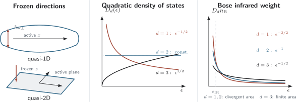
Strong confinement freezes transverse motion and leaves a tube-like quasi-1D gas or a plane-like quasi-2D gas. For quadratic dispersion, $D_1(\epsilon)\propto\epsilon^{-1/2}$ and $D_2(\epsilon)$ is constant. Multiplication by the low-energy Bose factor $n_{\mathrm B}(\epsilon)\sim(k_{\mathrm B}T)/\epsilon$ makes the excited-state integral infrared divergent for $d=1,2$, whereas the $d=3$ singularity remains integrable.

Thermal Wavelength and Phase-Space Density

The thermal de Broglie wavelength is dimension independent as a length,

$$\lambda_T = \sqrt{ \frac{2\pi\hbar^2}{mk_{\mathrm B}T} }.$$

What changes is the dimensionless degeneracy parameter. If $n_d=N/V_d$, then

$$\mathcal D_d = \frac{n_d\lambda_T^d}{g}.$$

Thus the relevant combinations are $n_1\lambda_T/g$ in one dimension and $n_2\lambda_T^2/g$ in two dimensions. Quantum statistics becomes important when $\mathcal D_d$ is not small. This criterion diagnoses degeneracy, not condensation: a uniform two-dimensional Bose gas can be deeply degenerate even though its ideal thermodynamic limit has no finite-temperature Bose–Einstein transition.

For fugacity

$$z = e^{\beta\mu}, \qquad \beta = \frac{1}{k_{\mathrm B}T},$$

the uniform ideal-gas number equations are

$$n_d^{(\mathrm B)} = \frac{g}{\lambda_T^d} \operatorname{Li}_{d/2}(z), \qquad 0<z\le 1,$$

and

$$n_d^{(\mathrm F)} = -\frac{g}{\lambda_T^d} \operatorname{Li}_{d/2}(-z), \qquad z>0.$$

These equations follow by integrating the Bose–Einstein or Fermi–Dirac occupation against $D_d(\epsilon)$. Their order, $d/2$, is a direct imprint of spatial dimension.

The Bose Infrared Obstruction

At a putative ideal-gas condensation threshold, the chemical potential approaches the one-particle ground energy. Taking that energy to be zero,

$$\mu \to 0^-.$$

For $\epsilon\ll k_{\mathrm B}T$,

$$\frac{1}{e^{\beta\epsilon}-1} \simeq \frac{k_{\mathrm B}T}{\epsilon}.$$

The low-energy contribution to the excited density therefore scales as

$$n_{\mathrm{ex}} \sim \int_0 d\epsilon\, \epsilon^{d/2-2}.$$

The lower limit converges only if

$$d > 2.$$

For a uniform ideal gas with quadratic dispersion:

• in $d=1$, the integrand behaves as $\epsilon^{-3/2}$;
• in $d=2$, it behaves as $\epsilon^{-1}$ and diverges logarithmically;
• in $d=3$, it behaves as $\epsilon^{-1/2}$ and is integrable.

The failure in one and two dimensions is not a shortage of low-energy states. It is the opposite: the combined low-energy state density and Bose enhancement allow the excited modes to absorb arbitrarily many particles as the system grows. There is no finite excited-state capacity that forces a macroscopic population into one mode.

The Bose–Einstein Condensation page gives the general density-of-states criterion and owns the full transition derivation. Here the result serves as the first signal that low-dimensional thermodynamic limits are infrared sensitive.

Exact Two-Dimensional Ideal Bose Relation

Two dimensions provide an especially transparent example because

$$\operatorname{Li}_1(z) = -\ln(1-z).$$

The number equation is

$$\frac{n_2\lambda_T^2}{g} = -\ln(1-z).$$

At any finite density and nonzero temperature,

$$z = 1 - \exp\left( -\frac{n_2\lambda_T^2}{g} \right) < 1.$$

Consequently,

$$\mu = k_{\mathrm B}T \ln\left[ 1 - \exp\left( -\frac{n_2\lambda_T^2}{g} \right) \right] < 0.$$

As the gas becomes highly degenerate, $\mu$ approaches zero exponentially closely but does not reach it at finite $T$ in the uniform thermodynamic limit. A finite experimental resolution can therefore make a strongly degenerate ideal gas look threshold-like even when no exact phase transition exists.

One-Dimensional Ideal Bose Asymptotics

In one dimension,

$$n_1 = \frac{g}{\lambda_T} \operatorname{Li}_{1/2}(z).$$

Write

$$z = e^{-\alpha}, \qquad \alpha = -\beta\mu > 0.$$

As $\alpha\to0^+$,

$$\operatorname{Li}_{1/2}(e^{-\alpha}) \simeq \sqrt{\frac{\pi}{\alpha}} + \zeta(1/2) + O(\sqrt{\alpha}).$$

Keeping the leading term gives

$$\alpha \simeq \frac{\pi g^2}{n_1^2\lambda_T^2},$$

and hence

$$\mu \simeq -\frac{g^2m(k_{\mathrm B}T)^2}{2\hbar^2n_1^2}.$$

The chemical potential again remains negative at every nonzero temperature. Its algebraic approach to zero is different from the exponentially small two-dimensional result, reflecting the stronger one-dimensional infrared divergence.

This asymptotic formula is for a uniform, ideal continuum gas at fixed line density. It is not an equation of state for an interacting one-dimensional Bose fluid.

Finite Size Is Not a Thermodynamic Transition

A finite box has a lowest nonzero excitation energy. For a periodic length $L$,

$$\epsilon_L \sim \frac{\hbar^2}{2m} \left( \frac{2\pi}{L} \right)^2.$$

This energy acts as an infrared cutoff. The excited population is then finite at $\mu=0$, and a rapid increase of ground-mode occupation can occur as temperature or particle number is varied.

The cutoff disappears as $L\to\infty$. In two dimensions the maximum excited density grows logarithmically with system size,

$$n_{\mathrm{ex,max}}^{(2)} \sim \frac{g}{\lambda_T^2} \ln\left( \frac{k_{\mathrm B}T}{\epsilon_L} \right),$$

up to geometry-dependent constants. In one dimension it grows more strongly. Therefore the apparent threshold drifts with size rather than approaching a nonzero bulk critical temperature.

Three observations must be kept separate:

• a single mode can be highly occupied in a finite sample;
• a finite sample can have a long coherence length compared with its size;
• a thermodynamic phase transition requires a specified infinite-system limit and nonanalytic bulk behavior.

The Thermodynamic Limit page develops that distinction systematically.

Fermi Seas in One and Two Dimensions

Fermions do not have the same excited-state-capacity problem. At zero temperature, all one-particle states are filled up to $k_{\mathrm F}$, with at most one fermion per internal state and momentum mode.

In one dimension, the occupied region is the interval

$$-k_{\mathrm F} \le k \le k_{\mathrm F}.$$

Counting both Fermi points gives

$$n_1 = \frac{gk_{\mathrm F}}{\pi},$$

so

$$k_{\mathrm F}^{(1)} = \frac{\pi n_1}{g},$$

and

$$\epsilon_{\mathrm F}^{(1)} = \frac{\hbar^2\pi^2n_1^2}{2mg^2}.$$

In two dimensions, the occupied region is a disk. Its area is $\pi k_{\mathrm F}^2$, so

$$n_2 = \frac{gk_{\mathrm F}^2}{4\pi},$$

and

$$k_{\mathrm F}^{(2)} = \sqrt{\frac{4\pi n_2}{g}}.$$

The corresponding Fermi energy is

$$\epsilon_{\mathrm F}^{(2)} = \frac{2\pi\hbar^2n_2}{mg}.$$

The one-dimensional Fermi surface consists of the two points $\pm k_{\mathrm F}$. The two-dimensional Fermi surface is a circle for an isotropic quadratic dispersion. These are boundaries in momentum space, not material surfaces in real space.

The Fermi Momentum and Fermi Energy page owns the general $d$-dimensional counting framework, while Fermi Surface develops the geometric and low-energy meaning of that boundary.

Zero-Temperature Fermi Thermodynamics

For a quadratic dispersion in $d$ dimensions,

$$\frac{E_0}{N} = \frac{d}{d+2} \epsilon_{\mathrm F},$$

and scale invariance gives

$$P_0V_d = \frac{2}{d}E_0.$$

Thus a one-dimensional ideal Fermi gas obeys

$$\frac{E_0}{N} = \frac{\epsilon_{\mathrm F}}{3}, \qquad P_0 = \frac{2}{3}n_1\epsilon_{\mathrm F},$$

where one-dimensional pressure has units of force. In two dimensions,

$$\frac{E_0}{N} = \frac{\epsilon_{\mathrm F}}{2}, \qquad P_0 = \frac{1}{2}n_2\epsilon_{\mathrm F}.$$

At low temperature, the ideal-gas heat capacity is

$$\frac{C_V}{Nk_{\mathrm B}} = \frac{\pi^2d}{6} \frac{T}{T_{\mathrm F}} + O\left( \frac{T^3}{T_{\mathrm F}^3} \right),$$

provided the Fermi energy lies well away from a singular band edge and the density of states is smooth over the thermal window. In one dimension this condition matters because $D_1(\epsilon)$ diverges at zero energy.

A Special Two-Dimensional Fermi Identity

Because the two-dimensional quadratic density of states is constant, the number equation can be inverted exactly:

$$n_2 = \frac{g}{\lambda_T^2} \ln(1+z).$$

Using

$$\frac{n_2\lambda_T^2}{g} = \frac{\epsilon_{\mathrm F}}{k_{\mathrm B}T},$$

one obtains

$$\mu(T) = k_{\mathrm B}T \ln\left( e^{\epsilon_{\mathrm F}/k_{\mathrm B}T} - 1 \right).$$

Equivalently,

$$\mu(T) = \epsilon_{\mathrm F} + k_{\mathrm B}T \ln\left( 1-e^{-\epsilon_{\mathrm F}/k_{\mathrm B}T} \right).$$

The low-temperature correction is exponentially small. A naive power-series Sommerfeld shift vanishes because $D_2'(\epsilon)=0$. The Sommerfeld Expansion page explains why this does not mean that every thermal correction vanishes.

Number Fluctuations Grow in the Infrared

In the grand canonical ensemble,

$$\operatorname{Var}(N) = k_{\mathrm B}T \left( \frac{\partial N}{\partial\mu} \right)_{T,V_d}.$$

For a uniform ideal Bose gas above any finite-size crossover,

$$\frac{\operatorname{Var}(N)}{N} = \frac{ \operatorname{Li}_{d/2-1}(z) }{ \operatorname{Li}_{d/2}(z) }.$$

As $z\to1^-$, the numerator weights the infrared modes even more strongly than the density does. In two dimensions it contains

$$\operatorname{Li}_0(z) = \frac{z}{1-z},$$

and in one dimension it contains $\operatorname{Li}_{-1/2}(z)$. Both diverge strongly. Low-dimensional ideal Bose gases are therefore highly compressible and fluctuation sensitive in the degenerate regime.

This formula describes total-number fluctuations in a grand canonical ideal gas. Fluctuations in a finite imaging cell, a canonical sample, or an interacting fluid require the appropriate correlation function and ensemble. It would be a mistake to infer a literal laboratory variance without matching those conditions.

Fermi occupation fluctuations instead contain $f(1-f)$. Pauli blocking suppresses fluctuations deep inside the filled sea, leaving a thermal shell near the Fermi boundary. Low dimension still changes the available phase space, but it does not create the Bose infrared pileup.

Long-Wavelength Phase Fluctuations

State counting explains the ideal gas. Interacting low-dimensional fluids add a second infrared mechanism: collective phase fluctuations.

Suppose amplitude fluctuations are weak enough that a bosonic field can be written locally as

$$\psi(\mathbf r) \simeq \sqrt{n_s} e^{i\theta(\mathbf r)}.$$

At long wavelengths, a phase-only free energy has the form

$$F_\theta = \frac{\hbar^2n_s}{2m} \int d^dr\, |\boldsymbol\nabla\theta|^2,$$

where $n_s$ is the superfluid number density in the active dimension. Thermal equipartition then gives the schematic variance

$$\left\langle [\theta(\mathbf r)-\theta(\mathbf 0)]^2 \right\rangle = \frac{2mk_{\mathrm B}T}{\hbar^2n_s} \int\frac{d^dk}{(2\pi)^d} \frac{1-\cos(\mathbf k\cdot\mathbf r)}{k^2}.$$

The integral has different infrared behavior in each dimension:

Dimension	Long-distance phase variance	Phase-only coherence
$d=1$	proportional to $\lvert x\rvert$ at $T>0$	exponential decay
$d=2$	proportional to $\ln r$ in the vortex-bound regime	algebraic decay
$d=3$	approaches a finite infrared contribution	true long-range phase order can survive

In one dimension, the Gaussian phase theory gives

$$\left\langle [\theta(x)-\theta(0)]^2 \right\rangle \simeq \frac{mk_{\mathrm B}T}{\hbar^2n_s}|x|,$$

and therefore

$$g^{(1)}(x) \propto \exp\left( -\frac{|x|}{\ell_\phi} \right), \qquad \ell_\phi = \frac{2\hbar^2n_s}{mk_{\mathrm B}T},$$

within this simple phase-only approximation.

In two dimensions,

$$\left\langle [\theta(\mathbf r)-\theta(\mathbf 0)]^2 \right\rangle \simeq \frac{mk_{\mathrm B}T}{\pi\hbar^2n_s} \ln\left( \frac{r}{a} \right),$$

so

$$g^{(1)}(r) \propto \left( \frac{a}{r} \right)^\eta, \qquad \eta = \frac{mk_{\mathrm B}T}{2\pi\hbar^2n_s}.$$

Here $a$ is a short-distance cutoff. Vortices, density fluctuations, scale dependence of $n_s$, and finite geometry must be added for a full theory. The Correlation Functions Overview page owns the general interpretation of exponential, algebraic, and long-range correlation behavior.

What the Hohenberg Result Says

Hohenberg used a Bogoliubov inequality to exclude ordinary finite-temperature long-range order for broad classes of homogeneous one- and two-dimensional Bose and Fermi systems with sufficiently short-range interactions. For a Bose fluid, the result formalizes the destructive role of long-wavelength fluctuations.

The hypotheses matter. The result does not say that:

• every finite low-dimensional cloud lacks a large coherent mode;
• two-dimensional superfluidity is impossible;
• discrete symmetries cannot order in two dimensions;
• long-range interactions obey the same conclusion without further analysis;
• a harmonic trap has the same density of states as a uniform box;
• zero-temperature quantum phases are covered by a finite-temperature theorem.

It is therefore safer to state the result with its physical setting than to invoke “the Mermin–Wagner theorem” as a universal slogan. Hohenberg’s continuum-fluid argument, the Mermin–Wagner spin result, and later generalizations are related but not interchangeable statements.

Two Dimensions and the BKT Preview

An interacting two-dimensional Bose fluid can be superfluid without possessing a nonzero infinite-distance limit of $g^{(1)}(r)$. In the low-temperature phase, vortex–antivortex pairs are bound and correlations decay algebraically. At the Berezinskii–Kosterlitz–Thouless transition, free vortices proliferate and correlations become short ranged.

For a homogeneous bosonic fluid, the universal jump can be written as

$$\frac{\hbar^2n_s(T_{\mathrm{BKT}}^-)}{m} = \frac{2k_{\mathrm B}T_{\mathrm{BKT}}}{\pi}.$$

Equivalently,

$$n_s(T_{\mathrm{BKT}}^-) \lambda_{T_{\mathrm{BKT}}}^2 = 4.$$

This is a statement about the renormalized long-wavelength superfluid density just below the transition, not the total density and not a generic finite trapped cloud. In an inhomogeneous trap, local critical behavior is rounded into a crossover and interpreted with finite-size and local-density analysis.

The key distinction is

$$\text{Bose–Einstein condensation} \ne \text{superfluidity} \ne \text{BKT quasi-long-range order}.$$

These notions can coexist in some systems, but none is a definition of the others.

One Dimension and the Luttinger-Liquid Preview

In one dimension, particles cannot pass one another without meeting. This kinematic fact magnifies the consequences of short-range interactions and makes collective descriptions unusually powerful.

A canonical continuum model is the repulsive contact Bose gas,

$$H = \int dx\, \left[ \frac{\hbar^2}{2m} (\partial_x\psi^\dagger) (\partial_x\psi) + \frac{g_{1\mathrm D}}{2} \psi^\dagger\psi^\dagger\psi\psi \right].$$

Its dimensionless interaction parameter is

$$\gamma = \frac{mg_{1\mathrm D}}{\hbar^2n_1}.$$

At fixed coupling, lowering the line density increases $\gamma$. The dilute limit can therefore be strongly correlated rather than more ideal. The weakly interacting regime and the strongly repulsive Tonks–Girardeau regime are separated by a continuous crossover in this model; Lieb–Liniger Model Preview owns the exact finite-coupling spectrum, thermodynamics, observables, and benchmark.

For broad classes of gapless one-dimensional interacting systems, the low-energy degrees of freedom are collective density and phase waves rather than long-lived particle-like excitations at a Fermi surface. A Luttinger-liquid description organizes correlation exponents through a sound velocity and a dimensionless interaction parameter. It also predicts phenomena such as spin–charge separation in suitable multicomponent fermion systems.

This is an orientation, not a derivation. Luttinger Liquid Preview owns bosonization, the effective Hamiltonian, correlation exponents, perturbations, and breakdown conditions.

Effective Interactions After Confinement

Freezing transverse motion does not justify carrying a three-dimensional contact coupling into a lower-dimensional Hamiltonian unchanged.

Let the three-dimensional field approximately factorize as

$$\Psi(\mathbf r) \simeq \phi_\perp(\mathbf r_\perp) \psi(x)$$

for a quasi-one-dimensional gas. A simple projection of a weak three-dimensional contact interaction gives

$$g_{1\mathrm D}^{(\mathrm{proj})} = g_{3\mathrm D} \int d^2r_\perp\, |\phi_\perp(\mathbf r_\perp)|^4.$$

For a harmonic transverse ground state with oscillator length

$$a_\perp = \sqrt{\frac{\hbar}{m\omega_\perp}},$$

this projection yields

$$g_{1\mathrm D}^{(\mathrm{proj})} = \frac{g_{3\mathrm D}}{2\pi a_\perp^2}.$$

Similarly, a quasi-two-dimensional projection gives

$$g_{2\mathrm D}^{(\mathrm{proj})} = g_{3\mathrm D} \int dz\, |\phi_0(z)|^4 = \frac{g_{3\mathrm D}}{\sqrt{2\pi}a_z}$$

for a harmonic ground mode with length $a_z$.

These projected formulas are only leading weak-coupling estimates. Exact low-energy scattering includes virtual transverse excitations. In quasi-one-dimensional geometry this produces a confinement-induced resonance; in two dimensions the effective scattering amplitude depends logarithmically on collision energy or density. The coupling must therefore be matched to the actual confinement and scattering convention before quantitative use.

Uniform and Trapped Dimensionality Are Different Questions

Changing the external potential changes the density of states independently of changing spatial dimension.

For a $d$-dimensional harmonic trap in the semiclassical regime,

$$D_{\mathrm{trap},d}(\epsilon) \propto \epsilon^{d-1}.$$

The ideal Bose excited-state integral then has low-energy behavior

$$\int_0 d\epsilon\, \epsilon^{d-2}.$$

A two-dimensional harmonic trap has a finite semiclassical excited-state capacity and can support an ideal-gas condensation transition in its appropriate trap thermodynamic limit. A one-dimensional harmonic trap is marginal and retains a logarithmic divergence in the standard limit.

This does not contradict the uniform result. The box and the trap are different sequences of spectra. A finite trapped gas also rounds any sharp limiting singularity.

The Quantum Gases in Traps page owns harmonic spectra, local-density profiles, imaging observables, and the trap thermodynamic limit.

Dimensional Crossover in Practice

Suppose a three-dimensional harmonic trap has frequencies

$$\omega_x \ll \omega_y, \omega_z.$$

If

$$k_{\mathrm B}T, \epsilon_{\mathrm F}, \mu_{\mathrm{int}}, \hbar\omega_{\mathrm{probe}} \ll \hbar\omega_y, \hbar\omega_z,$$

then motion is effectively one dimensional along $x$. For a quasi-two-dimensional gas, only one direction needs to be frozen.

The inequalities are not sharp phase boundaries. As an active scale approaches a transverse gap:

• excited transverse subbands acquire thermal population;
• the density of states develops step-like or threshold structure;
• scattering can couple open and closed transverse channels;
• thermodynamic observables cross over continuously between dimensions;
• local dimensionality can vary across an inhomogeneous cloud.

A reliable dimensionality claim should state the confinement frequencies and compare them with all relevant energy scales. A cloud aspect ratio alone is insufficient evidence.

Experimental Signatures

Low-dimensional atomic gases are commonly produced with anisotropic magnetic or optical confinement, atom-chip waveguides, or optical lattices that form arrays of tubes or planes.

Useful observables include:

• transverse populations: spectroscopy or thermometry can test whether excited frozen modes are occupied;
• in-situ density profiles: an equation of state reveals the dimension-dependent density of states and compressibility;
• momentum distributions: narrow central features diagnose long coherence lengths but do not alone prove true condensation;
• interference correlations: algebraic or exponential coherence can be distinguished over an accessible range;
• density correlations: bunching, antibunching, and local pair suppression probe statistics and interaction strength;
• collective modes: dimensional crossover and scale anomalies modify breathing and sound modes;
• vortex statistics: bound pairs and free vortices are central signatures of two-dimensional BKT physics.

Landmark cold-atom experiments realized strongly correlated one-dimensional bosons in optical tube arrays and observed BKT-type behavior in trapped two-dimensional Bose gases. Such experiments are finite, inhomogeneous, and measured over finite dynamic range. Their comparison with homogeneous thermodynamic statements therefore requires the physical audit in Finite-Size Effects together with trap-specific and imaging analysis.

Common Mistakes

Calling every elongated trap one dimensional

Geometry is not enough. Compare temperature, interaction, Fermi, and drive energies with the transverse gap.

Reusing three-dimensional densities

A line density, area density, and volume density have different units. So do their pressures and couplings.

Concluding that no BEC means no degeneracy

The phase-space density $n_d\lambda_T^d/g$ can be large in one or two dimensions even without a uniform ideal-gas condensation transition.

Concluding that no BEC means no superfluidity

An interacting two-dimensional gas can have BKT superfluidity and algebraic order without ordinary long-range one-body order.

Treating a finite-size crossover as a bulk transition

Large ground-mode occupation or system-wide coherence in a finite cloud does not by itself establish a nonanalytic thermodynamic limit.

Applying the Hohenberg or Mermin–Wagner name without hypotheses

Dimension, temperature, interaction range, symmetry, homogeneity, and the observable called “order” all matter.

Assuming weak density means weak interactions in one dimension

For the Lieb–Liniger parameter $\gamma=mg_{1\mathrm D}/(\hbar^2n_1)$, lowering density strengthens the dimensionless interaction.

Using a projected coupling as an exact coupling

Virtual transverse excitations renormalize low-dimensional scattering and can generate confinement-induced resonances.

Treating Fermi points as ordinary quasiparticle surfaces

The ideal one-dimensional gas has Fermi points, but interactions can replace the Landau-quasiparticle picture with Luttinger-liquid collective modes.

Summary

For quadratic continuum particles,

$$\frac{D_d(\epsilon)}{V_d} = \frac{g}{\Gamma(d/2)} \left( \frac{m}{2\pi\hbar^2} \right)^{d/2} \epsilon^{d/2-1}.$$

The main consequences are:

• $D_1(\epsilon)\propto\epsilon^{-1/2}$, while $D_2(\epsilon)$ is constant;
• a uniform ideal Bose gas with quadratic dispersion has no finite-temperature condensation transition for $d\le2$;
• finite systems and traps can show strong occupation crossovers, and a two-dimensional harmonic trap changes the ideal condensation criterion;
• one-dimensional Fermi seas terminate at two Fermi points, while two-dimensional isotropic seas have circular boundaries;
• thermal and phase fluctuations are enhanced at long wavelength;
• interacting two-dimensional Bose fluids can undergo a BKT transition without ordinary long-range order;
• generic gapless one-dimensional interacting fluids lead toward Luttinger-liquid behavior;
• effective dimension and effective coupling must both be derived from the confinement scales.

Low-Dimensional Quantum Matter places these gas results in the broader materials ledger of subband occupancy, environmental dimension, electronic platforms, disorder, and dimensionality evidence.

Exercises

Exercise 1: Derive the density of states

Starting from periodic momentum quantization, derive $D_d(\epsilon)/V_d$ for quadratic dispersion. Verify the explicit one- and two-dimensional formulas, including all factors of $2$, $\pi$, and $\hbar$.

Solution

The number of states inside a $d$-dimensional momentum sphere is

$$\mathcal N_d(k) = g\frac{V_d}{(2\pi)^d} \frac{S_{d-1}}{d}k^d.$$

Using $S_{d-1}=2\pi^{d/2}/\Gamma(d/2)$ and $k=\sqrt{2m\epsilon}/\hbar$ gives

$$\frac{\mathcal N_d(\epsilon)}{V_d} = \frac{g}{\Gamma(d/2+1)} \left( \frac{m}{2\pi\hbar^2} \right)^{d/2} \epsilon^{d/2}.$$

Differentiation yields

$$\frac{D_d(\epsilon)}{V_d} = \frac{g}{\Gamma(d/2)} \left( \frac{m}{2\pi\hbar^2} \right)^{d/2} \epsilon^{d/2-1}.$$

For $d=1$, $\Gamma(1/2)=\sqrt\pi$, so

$$\frac{D_1}{L} = \frac{g}{\pi\hbar} \sqrt{\frac{m}{2\epsilon}}.$$

For $d=2$, $\Gamma(1)=1$, giving

$$\frac{D_2}{A} = \frac{gm}{2\pi\hbar^2}.$$

Exercise 2: Infrared convergence for a general dispersion

Let $\epsilon_{\mathbf k}=Ak^s$ at small $k$, with $A>0$. Determine the condition on $d$ and $s$ for a uniform ideal Bose gas to have finite excited-state capacity at nonzero temperature.

Solution

The number of states below $k$ scales as $k^d$. Since $k\propto\epsilon^{1/s}$,

$$D(\epsilon) \propto \epsilon^{d/s-1}.$$

At $\mu=0$, the Bose factor is proportional to $1/\epsilon$ at low energy. The excited-state integrand is therefore

$$D(\epsilon)n_{\mathrm B}(\epsilon) \propto \epsilon^{d/s-2}.$$

The integral at zero converges when its exponent is greater than $-1$:

$$\frac{d}{s}-2 > -1.$$

Hence

$$d > s.$$

For $s=2$, this reduces to $d>2$.

Exercise 3: Invert the two-dimensional Bose number equation

For a uniform ideal Bose gas in two dimensions, derive $z(n_2,T)$ and $\mu(n_2,T)$. Find the leading highly degenerate asymptotic form of $\mu$.

Solution

Using $\operatorname{Li}_1(z)=-\ln(1-z)$,

$$\frac{n_2\lambda_T^2}{g} = -\ln(1-z).$$

Exponentiating gives

$$z = 1 - e^{-n_2\lambda_T^2/g}.$$

Therefore

$$\mu = k_{\mathrm B}T \ln\left( 1-e^{-n_2\lambda_T^2/g} \right).$$

When $n_2\lambda_T^2/g\gg1$, use $\ln(1-x)\simeq-x$:

$$\mu \simeq -k_{\mathrm B}T \exp\left( -\frac{n_2\lambda_T^2}{g} \right).$$

It is exponentially close to zero but remains negative at finite temperature.

Exercise 4: One- and two-dimensional Fermi scales

Derive $k_{\mathrm F}$, $\epsilon_{\mathrm F}$, and $E_0/N$ for uniform ideal Fermi gases in one and two dimensions with internal multiplicity $g$.

Solution

In one dimension, the occupied interval has length $2k_{\mathrm F}$:

$$n_1 = g\frac{2k_{\mathrm F}}{2\pi} = \frac{gk_{\mathrm F}}{\pi}.$$

Thus

$$k_{\mathrm F} = \frac{\pi n_1}{g}, \qquad \epsilon_{\mathrm F} = \frac{\hbar^2\pi^2n_1^2}{2mg^2}.$$

Integrating the quadratic energy symmetrically from $-k_{\mathrm F}$ to $k_{\mathrm F}$ gives

$$\frac{E_0}{N} = \frac{\epsilon_{\mathrm F}}{3}.$$

In two dimensions,

$$n_2 = g\frac{\pi k_{\mathrm F}^2}{(2\pi)^2} = \frac{gk_{\mathrm F}^2}{4\pi}.$$

Hence

$$k_{\mathrm F} = \sqrt{\frac{4\pi n_2}{g}}, \qquad \epsilon_{\mathrm F} = \frac{2\pi\hbar^2n_2}{mg}.$$

The constant density of states gives

$$\frac{E_0}{N} = \frac{\epsilon_{\mathrm F}}{2}.$$

Exercise 5: Phase fluctuations in one dimension

Evaluate

$$I(x) = \int_{-\infty}^{\infty} \frac{dk}{2\pi} \frac{1-\cos(kx)}{k^2}.$$

Use it to recover the phase-only coherence length $\ell_\phi$.

Solution

Differentiate with respect to $|x|$, or use the standard Fourier integral:

$$I(x) = \frac{|x|}{2}.$$

Substitution into

$$\left\langle [\theta(x)-\theta(0)]^2 \right\rangle = \frac{2mk_{\mathrm B}T}{\hbar^2n_s}I(x)$$

gives

$$\left\langle [\theta(x)-\theta(0)]^2 \right\rangle = \frac{mk_{\mathrm B}T}{\hbar^2n_s}|x|.$$

For Gaussian phase fluctuations,

$$\left\langle e^{i[\theta(x)-\theta(0)]} \right\rangle = \exp\left[ -\frac{1}{2} \left\langle [\theta(x)-\theta(0)]^2 \right\rangle \right].$$

Therefore

$$g^{(1)}(x) \propto e^{-|x|/\ell_\phi}, \qquad \ell_\phi = \frac{2\hbar^2n_s}{mk_{\mathrm B}T}.$$

Exercise 6: Uniform plane versus harmonic plane

Explain why a uniform two-dimensional ideal Bose gas lacks a finite-temperature condensation transition while a semiclassical two-dimensional harmonic trap can have finite excited-state capacity.

Solution

For the uniform quadratic gas,

$$D_{\mathrm{box},2}(\epsilon) \propto \epsilon^0.$$

At $\mu=0$, multiplication by the Bose factor gives an integrand proportional to $\epsilon^{-1}$, which diverges logarithmically.

For a two-dimensional harmonic trap, semiclassical phase-space counting gives

$$D_{\mathrm{trap},2}(\epsilon) \propto \epsilon.$$

The low-energy Bose integrand is then proportional to a constant, so its lower limit converges. The trap changes the spectrum and therefore the thermodynamic limit; it is not merely a boundary around the uniform gas.

Exercise 7: Test dimensional freezing

A gas has transverse frequency $\omega_\perp$ and active scales $k_{\mathrm B}T$, $\epsilon_{\mathrm F}$, $\mu_{\mathrm{int}}$, and $\hbar\omega_{\mathrm{drive}}$. Formulate a conservative dimensionless test for quasi-one-dimensional behavior. What conclusion follows if one ratio is of order unity?

Solution

Define

$$\eta_{\mathrm{dim}} = \frac{ \max( k_{\mathrm B}T, \epsilon_{\mathrm F}, |\mu_{\mathrm{int}}|, \hbar\omega_{\mathrm{drive}} ) }{ \hbar\omega_\perp }.$$

A conservative frozen-mode regime requires

$$\eta_{\mathrm{dim}} \ll 1.$$

If one ratio is of order unity, the corresponding process can populate or virtually mix transverse excitations. The system lies in a dimensional crossover for that observable or protocol, even if its equilibrium image remains highly elongated.

Exercise 8: Diagnose four claims

Classify each statement as correct, incorrect, or incomplete.

1. “A uniform two-dimensional ideal Bose gas cannot be quantum degenerate.”
2. “No finite-temperature BEC in two dimensions implies no two-dimensional superfluidity.”
3. “A finite one-dimensional gas may have coherence across the whole sample.”
4. “Projecting onto a transverse ground state always gives the exact effective coupling.”

Solution

1. Incorrect. The phase-space density $n_2\lambda_T^2/g$ can be arbitrarily large. The absent feature is a uniform ideal-gas thermodynamic condensation transition, not degeneracy.
2. Incorrect. An interacting two-dimensional Bose fluid can have BKT superfluidity with algebraic correlations and no ordinary infinite-distance condensate order.
3. Correct with finite-size qualification. If the coherence length exceeds the system size, the sample can appear globally coherent even though the corresponding infinite system has no finite-temperature long-range order.
4. Incorrect. Simple projection is a weak-coupling estimate. Virtual transverse excitation and low-dimensional scattering renormalize the coupling and can produce a confinement-induced resonance.

References

1. K. Huang, Statistical Mechanics, 2nd ed. (Wiley, 1987) — ideal quantum gases, density-of-states methods, and thermodynamic limits.
2. R. K. Pathria and P. D. Beale, Statistical Mechanics, 4th ed. (Academic Press, 2021) — Bose and Fermi functions in general dimension.
3. L. Pitaevskii and S. Stringari, Bose–Einstein Condensation and Superfluidity (Oxford University Press, 2016) — trapped gases, low-dimensional fluctuations, and superfluidity.
4. C. J. Pethick and H. Smith, Bose–Einstein Condensation in Dilute Gases, 2nd ed. (Cambridge University Press, 2008) — effective dimensionality and dilute-gas scales.
5. P. C. Hohenberg, “Existence of Long-Range Order in One and Two Dimensions”, Physical Review 158, 383–386 (1967) — Bogoliubov-inequality restrictions on finite-temperature long-range order.
6. V. L. Berezinskii, “Destruction of Long-Range Order in One-Dimensional and Two-Dimensional Systems Having a Continuous Symmetry Group,” Soviet Physics JETP 32, 493–500 (1971); 34, 610–616 (1972) — topological-defect mechanism and low-dimensional correlations.
7. J. M. Kosterlitz and D. J. Thouless, “Ordering, metastability and phase transitions in two-dimensional systems”, Journal of Physics C 6, 1181–1203 (1973) — vortex-unbinding transition.
8. D. R. Nelson and J. M. Kosterlitz, “Universal Jump in the Superfluid Density of Two-Dimensional Superfluids”, Physical Review Letters 39, 1201–1205 (1977) — universal superfluid-density jump.
9. E. H. Lieb and W. Liniger, “Exact Analysis of an Interacting Bose Gas. I. The General Solution and the Ground State”, Physical Review 130, 1605–1616 (1963) — exact repulsive one-dimensional contact Bose gas.
10. M. Girardeau, “Relationship between Systems of Impenetrable Bosons and Fermions in One Dimension”, Journal of Mathematical Physics 1, 516–523 (1960) — Bose–Fermi mapping in the hard-core limit.
11. M. Olshanii, “Atomic Scattering in the Presence of an External Confinement and a Gas of Impenetrable Bosons”, Physical Review Letters 81, 938–941 (1998) — confinement-induced renormalization and resonance in quasi-one-dimensional gases.
12. M. A. Cazalilla, R. Citro, T. Giamarchi, E. Orignac, and M. Rigol, “One dimensional bosons: From condensed matter systems to ultracold gases”, Reviews of Modern Physics 83, 1405–1466 (2011) — exact models, Luttinger liquids, and experiments.
13. V. Bagnato and D. Kleppner, “Bose–Einstein condensation in low-dimensional traps”, Physical Review A 44, 7439–7441 (1991) — how trapping modifies the dimensional condensation criterion.
14. B. Paredes et al., “Tonks–Girardeau gas of ultracold atoms in an optical lattice”, Nature 429, 277–281 (2004) — experimental realization of strongly correlated bosons in tube arrays.
15. T. Kinoshita, T. Wenger, and D. S. Weiss, “Observation of a One-Dimensional Tonks–Girardeau Gas”, Science 305, 1125–1128 (2004) — complementary one-dimensional hard-core-boson experiment.
16. Z. Hadzibabic, P. Krüger, M. Cheneau, B. Battelier, and J. Dalibard, “Berezinskii–Kosterlitz–Thouless crossover in a trapped atomic gas”, Nature 441, 1118–1121 (2006) — coherence and vortex signatures in a trapped two-dimensional Bose gas.
17. P. Krüger, Z. Hadzibabic, and J. Dalibard, “Critical Point of an Interacting Two-Dimensional Atomic Bose Gas”, Physical Review Letters 99, 040402 (2007) — critical atom number and the failure of an ideal-gas BEC description for an interacting 2D gas.