Low-Dimensional Quantum Matter

A quantum system is low dimensional when its relevant low-energy degrees of freedom propagate in fewer than three spatial directions. The definition is operational: a thin sample is not automatically two dimensional, and an anisotropic three-dimensional crystal is not automatically a stack of independent planes. The occupied transverse modes, probe energy, scattering rate, correlation length, interaction range, and coupling to the environment all matter.

Reducing dimension changes more than geometry. It changes how states accumulate near a band edge, how long-wavelength fluctuations build up, which scattering processes are kinematically special, how screening works, whether disorder interference remains infrared finite, and which topological structures are possible. These effects make one- and two-dimensional systems unusually fertile, but they do not imply that every low-dimensional system is strongly correlated or lacks order.

The durable questions are:

1. Which coordinates are dynamically active at the energy and length scale of the experiment?
2. Is the system strictly lower dimensional, quasi-low-dimensional, or in a crossover regime?
3. Which fields remain embedded in three dimensions even when the particles do not?
4. Which conclusion follows from dimension alone, and which needs symmetry, dispersion, interaction, or disorder assumptions?
5. What observation would reveal the return of an additional dimension?

Definition and Canonical Scope

This page is the canonical home for dimensionality as an organizing principle in quantum matter. It owns the distinction between geometric and effective dimension, the confinement and crossover criteria, the universal band-edge state-counting pattern, the infrared fluctuation argument, the generic interaction consequences, and an evidence ladder for dimensional claims.

Density of States owns detailed crystalline state counting, van Hove singularities, local and projected densities, and numerical methods. Low-Dimensional Quantum Gases owns ideal-gas thermodynamics, Bose infrared obstructions, and trapped-gas crossover. Luttinger Liquid Preview owns the one-dimensional interacting fixed point and bosonization dictionary. Scaling Theory of Localization owns dimensionless conductance and disorder-driven flow.

Device realizations have separate canonical homes: Quantum Wells for one-direction confinement, Quantum Wires for transverse modes and open channels, Quantum Dots for zero-dimensional addition spectra, and Two-Dimensional Electron Gases for populated interfaces and their transport diagnostics.

Why Dimension Matters

Dimension controls the phase space available to particles and collective modes. For an isotropic momentum shell of radius $k$, the number of states scales as $k^{d-1}dk$. For a long-wavelength mode with stiffness proportional to $q^2$, the fluctuation weight contains $d^dq/q^2$. The same integer $d$ therefore enters ultraviolet state counting and infrared stability in different ways.

Three broad changes recur:

• threshold structure: parabolic one-dimensional bands have inverse-square-root edge singularities, two-dimensional bands have steps, and three-dimensional bands turn on as a square root;
• infrared sensitivity: long-wavelength thermal fluctuations become progressively harder to suppress as $d$ decreases;
• kinematic restriction: conservation laws leave fewer independent scattering configurations, making special momenta such as $2k_F$ in one dimension unusually important.

Dimension also changes the mathematical objects available to phases. A two-dimensional gapped band can carry a Chern number and support a quantized Hall response. Two-dimensional configuration space permits anyonic exchange, while ordinary three-dimensional point particles have only bosonic or fermionic exchange classes. These are structural statements, not claims that topology appears in every two-dimensional material.

What Effective Dimension Means

Geometric dimension is only the first entry

Let a sample have macroscopic lengths $L_x$, $L_y$, and $L_z$. Its geometric dimension describes which lengths are large compared with microscopic structure. Its effective quantum dimension describes which directions support occupied and resolvable low-energy motion.

If motion in one or more directions is confined, a single-particle spectrum can often be organized as

$$E_{n,\mathbf k_\parallel} = E_n^\perp + \varepsilon_\parallel(\mathbf k_\parallel),$$

where $n$ labels transverse modes and $\mathbf k_\parallel$ labels motion along unconfined directions. Define the first transverse gap

$$\Delta_\perp = E_1^\perp-E_0^\perp.$$

A lowest-subband description requires both occupancy and resolution conditions. A useful sufficient ledger is

$$\begin{aligned} \mu-E_0^\perp,\quad k_BT,\quad \hbar\omega &\ll \Delta_\perp, \\ \Gamma,\quad e|V| &\ll \Delta_\perp, \end{aligned}$$

where $\Gamma$ is spectral broadening and $V$ is a bias relevant to the measurement. Not every term applies to every experiment, and the inequalities need not share one universal numerical threshold. The key point is that neither occupied states nor the probe should substantially access the next transverse mode.

Quasi-dimensional systems cross over

A layered tight-binding band illustrates a different route:

$$\varepsilon(\mathbf k) = \varepsilon_\parallel(k_x,k_y) -2t_\perp\cos(k_zc).$$

For $t_\perp=0$, the layers are kinematically independent. For any nonzero coherent $t_\perp$, the asymptotically low-energy Fermi surface is three dimensional, although an intermediate regime can look two dimensional. Whether interlayer motion is coherent also depends on broadening: the ratio $t_\perp/\Gamma$ is often as important as $t_\perp/k_BT$.

Critical behavior has its own crossover criterion. When an in-plane correlation length $\xi_\parallel$ exceeds a film thickness, fluctuations may first look two dimensional. Weak interlayer coupling can nevertheless restore three-dimensional critical behavior sufficiently close to a transition. “Two dimensional” must therefore name the observable and scale.

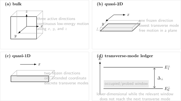
Effective dimension is fixed jointly by geometry, transverse-mode occupancy, and probe resolution. A slab or wire behaves as lower dimensional only while the relevant energies remain below $\Delta_\perp$; finite coupling or higher-mode access produces a dimensional crossover.

Four dimensions that should not be conflated

Dimension	Operational meaning	Typical diagnostic
geometric	number of macroscopically extended sample directions	microscopy, thickness, structure
kinematic	number of directions with active low-energy dispersion	subbands, Fermi-surface geometry, angular response
critical	dimension controlling long-distance fluctuations near a transition	finite-size and critical scaling
environmental	dimension in which mediating fields and reservoirs propagate	dielectric, phonon, photon, and substrate response

A two-dimensional electron gas can interact through a three-dimensional Coulomb field. A monolayer can hybridize with three-dimensional substrate phonons. A one-dimensional edge channel can be attached to macroscopic reservoirs. These mixed-dimensional problems are common, not pathological.

Density of States by Dimension

Parabolic threshold law

Consider one isotropic parabolic minimum,

$$E_{\mathbf k} = E_0+\frac{\hbar^2k^2}{2m^\ast},$$

with total internal degeneracy $g$ and $d$-dimensional measure $V_d$. Since each state occupies $(2\pi)^d/V_d$ in momentum space,

$$\begin{aligned} \frac{\nu_d(E)}{V_d} &= g\int \frac{d^dk}{(2\pi)^d} \delta(E-E_{\mathbf k}) \\ &= \frac{gS_{d-1}}{(2\pi)^d} \frac{m^\ast}{\hbar^2} \, k_E^{d-2} \Theta(E-E_0), \\ k_E &= \frac{\sqrt{2m^\ast(E-E_0)}}{\hbar}. \end{aligned}$$

where $S_{d-1}=2\pi^{d/2}/\Gamma(d/2)$ is the area of the unit $(d-1)$-sphere. The edge exponent is

$$\nu_d(E) \propto (E-E_0)^{d/2-1}\Theta(E-E_0).$$

The explicit results are:

$d$	DOS per $d$-dimensional measure	Band-edge behavior
1	$\dfrac{g}{\pi\hbar}\sqrt{\dfrac{m^\ast}{2(E-E_0)}}$	inverse-square-root divergence
2	$\dfrac{gm^\ast}{2\pi\hbar^2}$	constant step
3	$\dfrac{g}{4\pi^2}\left(\dfrac{2m^\ast}{\hbar^2}\right)^{3/2}\sqrt{E-E_0}$	square-root onset

In zero dimensions the continuum formula is replaced by discrete levels,

$$\nu_0(E) = \sum_j g_j\,\delta(E-E_j),$$

broadened in a real measurement by lifetime, temperature, and instrumental resolution.

Dimension does not determine the DOS alone

The threshold law assumes a quadratic isotropic extremum. For a $d$-dimensional Dirac cone,

$$E_\pm(\mathbf k) = E_D\pm\hbar v|\mathbf k|,$$

the DOS instead scales as $\nu_d(E)\propto |E-E_D|^{d-1}$. Saddle points produce van Hove singularities, nearly flat bands concentrate states into narrow energy windows, and anisotropic masses change prefactors.

Thus a DOS feature can support a dimensional assignment only after the dispersion, degeneracy, broadening, and matrix elements are controlled. A sharp one-dimensional subband edge is not, by itself, evidence for strong interactions.

Enhanced Fluctuations

The infrared phase integral

The simplest diagnostic uses a continuous order parameter with slowly varying phase $\theta(\mathbf r)$ and stiffness $\rho_s$:

$$F[\theta] = \frac{\rho_s}{2} \int d^dx\,|\nabla\theta|^2.$$

Classical equipartition gives

$$\left\langle |\theta_{\mathbf q}|^2\right\rangle = \frac{k_BT}{\rho_s q^2}.$$

Writing $\Delta\theta(\mathbf r)=\theta(\mathbf r)-\theta(\mathbf 0)$, the relative phase variance contains

$$\begin{aligned} \left\langle [\Delta\theta(\mathbf r)]^2 \right\rangle &= \frac{2k_BT}{\rho_s} \mathcal I_d(\mathbf r), \\ \mathcal I_d(\mathbf r) &= \int\frac{d^dq}{(2\pi)^d} \frac{1-\cos(\mathbf q\cdot\mathbf r)}{q^2}. \end{aligned}$$

At large $r$ its infrared contribution behaves schematically as

$$\left\langle[\Delta\theta(r)]^2\right\rangle \sim \begin{cases} r, & d=1,\\ \ln(r/a), & d=2,\\ \text{finite}, & d>2, \end{cases}$$

where $a$ is a microscopic cutoff. The growth in one and two dimensions is the spin-wave intuition behind the Hohenberg–Mermin–Wagner restrictions.

What the no-order theorem does and does not say

For equilibrium systems with sufficiently short-range interactions, the thermodynamic limit, and an exact continuous symmetry, thermal fluctuations prevent conventional spontaneous long-range order in one and two dimensions under the theorem’s hypotheses. The statement has important boundaries:

• it concerns nonzero temperature, not every zero-temperature quantum ground state;
• it does not forbid finite-temperature breaking of a discrete symmetry, as the two-dimensional Ising model demonstrates;
• it does not forbid algebraic correlations or a Berezinskii–Kosterlitz–Thouless transition;
• magnetic anisotropy, explicit symmetry breaking, long-range interactions, finite size, and interlayer coupling can change the conclusion;
• a large but finite correlation length can look ordered on a finite sample or within a finite observation time.

Saying “two-dimensional magnets cannot order” without these qualifiers is incorrect. Real monolayer magnets can order because spin–orbit coupling supplies anisotropy and removes the exact isotropic continuous symmetry assumed by the simplest theorem.

BKT order without a local order parameter

In an easy-plane or superfluid system, a vortex has the approximate energy and positional entropy

$$\begin{aligned} E_v &\simeq \pi\rho_s\ln\frac{L}{a}, \\ S_v &\simeq 2k_B\ln\frac{L}{a}. \end{aligned}$$

The single-vortex free-energy estimate changes sign when entropy can overcome stiffness. The full Berezinskii–Kosterlitz–Thouless theory treats interacting vortex pairs and renormalized stiffness; it predicts the universal jump

$$\rho_s(T_{\mathrm{BKT}}^-) = \frac{2}{\pi}k_BT_{\mathrm{BKT}}$$

when $\rho_s$ is expressed in energy units. Below the transition, correlations decay algebraically rather than approaching a nonzero constant. This is a distinct form of low-dimensional organization, not an exception that restores ordinary continuous-symmetry breaking.

Thermal and quantum dimensions differ

At a quantum critical point, imaginary time adds a scaling direction. If frequency scales as $\omega\sim q^z$, a common power-counting combination is

$$d_{\mathrm{eff}}^{\mathrm{critical}} = d+z.$$

This is a scaling relation, not permission to replace every $d$-dimensional quantum system by an isotropic classical system in $d+z$ dimensions. Conservation laws, long-range forces, damping, boundaries, and anisotropic scaling can alter the mapping. Quantum Criticality develops those qualifications.

Why Interactions Become More Consequential

Lower dimension does not automatically mean strong coupling

Interaction strength is always a ratio. Confinement can reduce kinetic phase space, weaken screening, or increase wave-function overlap, but a dilute interaction, large velocity, broad band, or strong dielectric environment can still leave a controlled weak-coupling regime.

For a conventional two-dimensional electron gas with areal density $n$,

$$\begin{aligned} a &= \frac{1}{\sqrt{\pi n}}, & a_B^\ast &= \frac{4\pi\epsilon\hbar^2}{m^\ast e^2}, & r_s &= \frac{a}{a_B^\ast}. \end{aligned}$$

Here $r_s$ compares a typical Coulomb scale with the Fermi kinetic scale up to convention-dependent constants. Lowering $n$ increases $r_s\propto n^{-1/2}$. This density scaling is not universal: for an ideal two-dimensional Dirac cone, the analogous coupling

$$\alpha_{\mathrm{eff}} = \frac{e^2}{4\pi\epsilon\hbar v_F}$$

is density independent before velocity renormalization and environmental effects are included.

One-dimensional kinematics reorganizes the low-energy theory

A one-dimensional Fermi sea has two Fermi points rather than a Fermi surface of finite dimension. Particle–hole response is singular near $2k_F$, and repeated forward and backward scattering cannot generally be summarized by long-lived electron-like quasiparticles. Generic gapless interacting one-dimensional fluids instead organize into collective density modes with interaction-dependent power laws.

This is the domain of the Luttinger-liquid description. It is powerful but not universal to every one-dimensional system: commensurability, disorder, spin gaps, confinement, long-range forces, or symmetry breaking can produce gapped or localized phases.

Confinement changes the interaction itself

Projecting a three-dimensional interaction into the lowest transverse mode gives a form-factor-dependent effective interaction,

$$\begin{aligned} V_{\mathrm{eff}}(\mathbf q_\parallel) &= \int dz\,dz'\, |\phi_0(z)|^2 \\ &\quad\times V(\mathbf q_\parallel;z,z') |\phi_0(z')|^2. \end{aligned}$$

The layer thickness, gates, substrate dielectric function, nearby metallic screening, and higher subbands all enter. A bare $1/r$ law should not be inserted into a strictly lower-dimensional model without specifying this embedding.

Large DOS and strong correlation are different claims

A divergent subband edge, van Hove singularity, or flat band enhances the number of low-energy states. It can amplify susceptibilities and make interactions more effective, but it does not identify the resulting phase. Disorder broadening may cut off the enhancement; matrix elements may suppress a channel; several orders may compete; and a large DOS can remain within a weak-coupling instability.

What Are Strong Correlations? supplies the separate evidence ledger for quasiparticle failure, spectral-weight transfer, local moments, and interaction-controlled scales.

Disorder, Topology, and Restricted Kinematics

Dimension also controls the return probability of a diffusing particle:

$$P(\mathbf 0,t) \propto (Dt)^{-d/2}.$$

The long-time interference correction involves $\int dt\,P(\mathbf0,t)$ and is increasingly infrared sensitive as $d$ decreases. This intuition underlies the special role of one and two dimensions in weak localization and one-parameter scaling. It does not mean every two-dimensional sample is experimentally insulating: finite dephasing, spin–orbit coupling, magnetic fields, topology, interactions, and symmetry class matter. The full statement belongs to Scaling Theory of Localization.

Restricted dimension can also stabilize responses with no direct three-dimensional analogue. The Integer Quantum Hall Effect uses a two-dimensional bulk and one-dimensional chiral boundary. The Fractional Quantum Hall Effect combines two-dimensional motion, magnetic flux, and interactions to produce fractionalized topological order. Dimensionality is necessary to these constructions but is not sufficient evidence for them.

Experimental Platforms

Platform	How motion is restricted	Strong dimensionality check
semiconductor quantum well or interface	band offsets confine one coordinate	occupied subbands, angle-dependent magnetotransport
semiconductor wire, nanotube, or atomic chain	transverse confinement leaves one extended coordinate	subband thresholds, channel counting, one-dimensional correlations
quantum dot	confinement in all three coordinates	discrete addition and excitation spectra
atomically thin crystal	one or a few covalently bonded layers	layer count plus electronic dispersion and thickness evolution
layered bulk crystal	weak interlayer hopping relative to in-plane hopping	$k_z$ dispersion, coherent crossover, transport and quantum-oscillation anisotropy
ultracold atomic pancake or tube	optical confinement freezes one or two oscillator directions	trap-frequency hierarchy and correlation scaling
superfluid or superconducting film	thickness below relevant coherence or screening lengths	stiffness, vortex response, thickness and finite-size scaling

The platform is not the conclusion. A monolayer is geometrically two dimensional, but its electrons, phonons, photons, substrate modes, and contacts can have different effective dimensions. A wire can contain many transverse subbands and behave as a multichannel quasi-one-dimensional metal. A layered crystal can cross from incoherent interlayer transport at high temperature to a coherent three-dimensional Fermi surface at low temperature.

Establishing Dimensionality

A claim ladder

Claim level	Evidence	What remains unresolved
geometric	thickness or aspect ratio	whether low-energy modes are frozen
spectral	resolved transverse subbands or dimensional DOS edge	interaction and coherence effects
kinematic	Fermi-surface shape, angular oscillations, channel count	many-body universality
collective	dimension-specific scaling, correlations, defects, or response	finite-size and crossover alternatives
crossover-controlled	systematic change with thickness, $T$, $\omega$, density, or $t_\perp$	residual model dependence

Transport anisotropy alone is weak evidence. A three-dimensional band can have strongly anisotropic masses or scattering times, while an ideal lower-dimensional channel can acquire apparent transverse response through contacts and leakage. Reliable assignments combine structure, spectroscopy, transport, and at least one controlled crossover.

Worked estimate: a GaAs quantum well

For an ideal well of width $L$ and effective mass $m^\ast$,

$$E_n^\perp = \frac{n^2\pi^2\hbar^2}{2m^\ast L^2}, \qquad n=1,2,\ldots$$

Taking $L=20\,\mathrm{nm}$ and $m^\ast=0.067m_e$ gives

$$\begin{aligned} E_1^\perp &\simeq 14\,\mathrm{meV}, \\ \Delta_\perp &= E_2^\perp-E_1^\perp \simeq 42\,\mathrm{meV}. \end{aligned}$$

If the in-plane Fermi energy is $8\,\mathrm{meV}$, $T=20\,\mathrm K$ gives $k_BT\simeq1.7\,\mathrm{meV}$, and $\Gamma\simeq0.5\,\mathrm{meV}$, then equilibrium low-energy transport is safely within the lowest-subband regime. An optical probe at $\hbar\omega=50\,\mathrm{meV}$ can access transverse excitations, so the same sample is not two dimensional for that measurement. Finite barriers and band nonparabolicity refine the numbers but not the logic.

Practical workflow

1. State the candidate active coordinates and the embedding environment.
2. List transverse gaps, chemical potential, temperature, frequency, bias, broadening, and interaction scales.
3. Verify mode occupancy with spectroscopy, capacitance, quantum oscillations, or threshold structure.
4. Test kinematics independently through angular dependence or momentum-resolved dispersion.
5. Search for the predicted dimensional crossover by tuning thickness, density, temperature, frequency, pressure, or interlayer coupling.
6. Only then assign dimension-specific many-body behavior.

Common Mistakes

• Equating thin with two dimensional. Thickness is geometric evidence; subband occupancy and probe scale establish kinematic dimension.
• Calling anisotropy dimensional reduction. A highly anisotropic three-dimensional dispersion still has three active momenta.
• Applying the parabolic DOS law to every band. Dirac cones, saddle points, flat bands, and disorder have different threshold structures.
• Overstating Hohenberg–Mermin–Wagner. The theorem has symmetry, interaction-range, temperature, and thermodynamic-limit assumptions.
• Treating BKT order as ordinary long-range order. Its low-temperature phase has algebraic correlations and bound vortices.
• Assuming low dimension guarantees strong correlation. Coupling ratios and screening must be evaluated.
• Ignoring the field environment. Lower-dimensional particles can interact through three-dimensional electromagnetic or elastic fields.
• Using one probe to define all regimes. A sample can be two dimensional for dc transport and three dimensional for a high-energy excitation.
• Ignoring finite size. A correlation length larger than the device can mimic order or hide an asymptotic crossover.

Exercises

Exercise 1: derive the band-edge exponent

Starting from $\nu_d(E)=gV_d\int d^dk\,(2\pi)^{-d}\delta(E-E_{\mathbf k})$, derive the DOS for an isotropic parabolic minimum in $d=1,2,3$. Check the physical units in each case.

Solution

Use $d^dk=S_{d-1}k^{d-1}dk$ and

$$\begin{aligned} \delta(E-E_{\mathbf k}) &= \frac{m^\ast}{\hbar^2k_E} \delta(k-k_E), \\ k_E &= \frac{\sqrt{2m^\ast(E-E_0)}}{\hbar}. \end{aligned}$$

Then

$$\frac{\nu_d(E)}{V_d} = \frac{gS_{d-1}}{(2\pi)^d} \frac{m^\ast}{\hbar^2} k_E^{d-2}\Theta(E-E_0).$$

Substituting $S_0=2$, $S_1=2\pi$, and $S_2=4\pi$ gives the three entries in the table above. Because $V_d$ has units of length$^d$, $\nu_d/V_d$ has units of energy$^{-1}$ length$^{-d}$.

Exercise 2: second-subband threshold

For the GaAs well in the worked estimate, take spin degeneracy $g=2$. At what areal density does the zero-temperature in-plane Fermi energy reach $\Delta_\perp=42\,\mathrm{meV}$? Use the ideal two-dimensional parabolic gas.

Solution

For total degeneracy $g$,

$$n = \frac{gk_F^2}{4\pi}, \qquad E_F = \frac{\hbar^2k_F^2}{2m^\ast} = \frac{2\pi\hbar^2n}{gm^\ast}.$$

With $g=2$,

$$n_{\mathrm{th}} = \frac{m^\ast\Delta_\perp}{\pi\hbar^2} \simeq 1.18\times10^{12}\,\mathrm{cm}^{-2}.$$

Near this density the second subband begins to populate in the ideal model. Temperature, disorder, electrostatic self-consistency, and finite barriers smear or shift the threshold.

Exercise 3: infrared phase fluctuations

Use power counting to determine whether $\int_{q_{\mathrm{IR}}}^{\Lambda}d^dq/q^2$ diverges as $q_{\mathrm{IR}}\to0$ for $d=1,2,3$. Explain why this integral is only an intuition for, not a complete proof of, the no-order theorem.

Solution

Angular integration leaves

$$I_d \propto \int_{q_{\mathrm{IR}}}^{\Lambda} dq\,q^{d-3}.$$

Thus

$$\begin{aligned} I_1&\propto q_{\mathrm{IR}}^{-1},\\ I_2&\propto \ln(\Lambda/q_{\mathrm{IR}}),\\ I_3&\propto \Lambda-q_{\mathrm{IR}}. \end{aligned}$$

The first two are infrared divergent, while the third is finite. This Gaussian phase argument identifies the dangerous soft modes but does not establish all theorem hypotheses, control vortices, handle amplitude fluctuations, or cover long-range interactions and explicit anisotropy. The rigorous Hohenberg and Mermin–Wagner results use inequalities tied to the microscopic symmetry and interactions.

Exercise 4: vortex free energy

Using the vortex energy and entropy estimates, find the temperature at which the coefficient of $\ln(L/a)$ changes sign. Why is the result not yet the exact BKT transition criterion?

Solution

The free energy is

$$F_v \simeq \left(\pi\rho_s-2k_BT\right) \ln\frac{L}{a}.$$

The bare estimate changes sign at $k_BT=\pi\rho_s/2$. Near the transition, however, vortex–antivortex pairs screen each other and renormalize the stiffness. The exact universal statement uses the long-distance renormalized stiffness evaluated just below the transition,

$$\rho_s(T_{\mathrm{BKT}}^-) = \frac{2k_BT_{\mathrm{BKT}}}{\pi}.$$

The two formulas are consistent only after distinguishing bare from renormalized quantities.

Exercise 5: density and interaction strength

Show that $r_s\propto n^{-1/2}$ for a parabolic two-dimensional electron gas with fixed $m^\ast$ and dielectric constant. Why does the same argument not give a density-dependent coupling for an ideal Dirac cone?

Solution

The mean spacing scales as $a\sim n^{-1/2}$. The Coulomb energy scales as $E_C\sim e^2/(\epsilon a)\propto n^{1/2}$, while the parabolic Fermi energy scales as $E_F\propto k_F^2/m^\ast\propto n$. Therefore

$$\frac{E_C}{E_F} \propto n^{-1/2},$$

which is the scaling of $r_s=a/a_B^\ast$. For a Dirac cone, $E_F\sim\hbar v_Fk_F\propto n^{1/2}$, the same density scaling as $E_C$. Their ratio is therefore the approximately density-independent $\alpha_{\mathrm{eff}}$, subject to velocity renormalization, screening, and band-curvature corrections.

Exercise 6: audit a dimensionality claim

A layered conductor has $\rho_c/\rho_{ab}=10^4$, and a paper calls it a two-dimensional metal. List three additional measurements or controls needed to make that claim convincing.

Solution

Resistivity anisotropy mixes band velocity and scattering-time anisotropy, so it is not sufficient. Useful independent checks include:

1. ARPES or quantum oscillations resolving negligible or finite $k_z$ dispersion;
2. angle-dependent magnetoresistance testing cylindrical versus warped three-dimensional orbits;
3. a temperature or pressure scan looking for coherent interlayer crossover;
4. optical conductivity comparing the interlayer bandwidth with $\Gamma$;
5. thickness dependence or subband structure in exfoliated samples.

The claim should also name the energy range: the same material may be quasi-two-dimensional above an interlayer coherence scale and three dimensional below it.

Key Takeaways

• Effective dimension is a scale-dependent property of active degrees of freedom, not a synonym for sample shape.
• The confinement gap must exceed occupancy, thermal, probe, bias, and broadening scales for a lowest-subband description.
• Parabolic band edges follow $\nu_d(E)\propto(E-E_0)^{d/2-1}$, but dispersion and critical points can override that simple pattern.
• Continuous-symmetry thermal fluctuations are infrared divergent in one and two dimensions under the Hohenberg–Mermin–Wagner assumptions; discrete order, BKT physics, finite size, anisotropy, and interlayer coupling require separate treatment.
• Reduced dimension can magnify interactions, disorder interference, and special kinematics, but none of those outcomes follows from dimension alone.
• A trustworthy dimensional assignment combines geometry, spectral modes, kinematics, collective behavior, and a controlled crossover.

Connections

• Quantum Matter Map places dimension among the structure, energy-scale, response, and evidence ledgers.
• Density of States develops constant-energy geometry, van Hove singularities, broadening, and experimental interpretation.
• Low-Dimensional Quantum Gases treats ideal Bose and Fermi gases, traps, and dimensional crossover in detail.
• Luttinger Liquid Preview develops the universal gapless one-dimensional interacting theory.
• Finite-Temperature Phase Transitions separates thermodynamic transitions, finite-size rounding, symmetry, and dimensional constraints.
• What Is Mesoscopic Physics? distinguishes confinement, coherence, mean-free-path, thermal, and contact scales.
• Two-Dimensional Materials applies the dimensional ledger to atomically thin crystals, environmental screening, valleys, excitons, and van der Waals assembly.
• 2D Magnets and Ferroelectrics applies the infrared fluctuation and crossover ledger to anisotropy-stabilized magnetic order, layer parity, and two-dimensional polar phases.
• Engineered Heterostructures shows how confinement, interface transfer, and dimensional crossover become design variables in superconducting, topological, oxide, and cavity hybrids.
• Quantum Materials by Design turns dimensionality, correlation, symmetry, synthesis, and robustness into explicit design coordinates.
• Two-Dimensional Electron Gases applies the scale ledger to populated semiconductor and oxide interfaces.
• Graphene and Dirac Materials shows how a two-dimensional Dirac dispersion changes state counting, pseudospin, and magnetic response.

Further Reading

For electronic platforms, begin with Ando, Fowler, and Stern, then compare Giamarchi’s one-dimensional treatment with the original Hohenberg–Mermin–Wagner and BKT papers. Geim and Grigorieva provide the materials bridge to atomically thin stacks, while Bloch, Dalibard, and Zwerger give a complementary route through tunable ultracold gases.

References

1. T. Ando, A. B. Fowler, and F. Stern, “Electronic Properties of Two-Dimensional Systems,” Reviews of Modern Physics 54, 437–672 (1982), doi:10.1103/RevModPhys.54.437.
2. N. D. Mermin and H. Wagner, “Absence of Ferromagnetism or Antiferromagnetism in One- or Two-Dimensional Isotropic Heisenberg Models,” Physical Review Letters 17, 1133–1136 (1966), doi:10.1103/PhysRevLett.17.1133.
3. P. C. Hohenberg, “Existence of Long-Range Order in One and Two Dimensions,” Physical Review 158, 383–386 (1967), doi:10.1103/PhysRev.158.383.
4. V. L. Berezinskii, “Destruction of Long-Range Order in One-Dimensional and Two-Dimensional Systems Having a Continuous Symmetry Group I. Classical Systems,” Soviet Physics JETP 32, 493–500 (1971), JETP archive.
5. J. M. Kosterlitz and D. J. Thouless, “Ordering, Metastability and Phase Transitions in Two-Dimensional Systems,” Journal of Physics C 6, 1181–1203 (1973), doi:10.1088/0022-3719/6/7/010.
6. D. R. Nelson and J. M. Kosterlitz, “Universal Jump in the Superfluid Density of Two-Dimensional Superfluids,” Physical Review Letters 39, 1201–1205 (1977), doi:10.1103/PhysRevLett.39.1201.
7. F. D. M. Haldane, “‘Luttinger Liquid Theory’ of One-Dimensional Quantum Fluids. I,” Journal of Physics C 14, 2585–2609 (1981), doi:10.1088/0022-3719/14/19/010.
8. T. Giamarchi, Quantum Physics in One Dimension (Oxford University Press, 2003), doi:10.1093/acprof:oso/9780198525004.001.0001.
9. E. Abrahams, P. W. Anderson, D. C. Licciardello, and T. V. Ramakrishnan, “Scaling Theory of Localization: Absence of Quantum Diffusion in Two Dimensions,” Physical Review Letters 42, 673–676 (1979), doi:10.1103/PhysRevLett.42.673.
10. L. Onsager, “Crystal Statistics. I. A Two-Dimensional Model with an Order-Disorder Transition,” Physical Review 65, 117–149 (1944), doi:10.1103/PhysRev.65.117.
11. K. S. Novoselov et al., “Electric Field Effect in Atomically Thin Carbon Films,” Science 306, 666–669 (2004), doi:10.1126/science.1102896.
12. K. S. Novoselov et al., “Two-Dimensional Atomic Crystals,” Proceedings of the National Academy of Sciences 102, 10451–10453 (2005), doi:10.1073/pnas.0502848102.
13. K. F. Mak, C. Lee, J. Hone, J. Shan, and T. F. Heinz, “Atomically Thin MoS₂: A New Direct-Gap Semiconductor,” Physical Review Letters 105, 136805 (2010), doi:10.1103/PhysRevLett.105.136805.
14. A. K. Geim and I. V. Grigorieva, “Van der Waals Heterostructures,” Nature 499, 419–425 (2013), doi:10.1038/nature12385.
15. Z. Hadzibabic, P. Krüger, M. Cheneau, B. Battelier, and J. Dalibard, “Berezinskii–Kosterlitz–Thouless Crossover in a Trapped Atomic Gas,” Nature 441, 1118–1121 (2006), doi:10.1038/nature04851.
16. I. Bloch, J. Dalibard, and W. Zwerger, “Many-Body Physics with Ultracold Gases,” Reviews of Modern Physics 80, 885–964 (2008), doi:10.1103/RevModPhys.80.885.
17. B. Huang et al., “Layer-Dependent Ferromagnetism in a van der Waals Crystal down to the Monolayer Limit,” Nature 546, 270–273 (2017), doi:10.1038/nature22391.
18. D. C. Tsui, H. L. Stormer, and A. C. Gossard, “Two-Dimensional Magnetotransport in the Extreme Quantum Limit,” Physical Review Letters 48, 1559–1562 (1982), doi:10.1103/PhysRevLett.48.1559.
19. D. J. Thouless, M. Kohmoto, M. P. Nightingale, and M. den Nijs, “Quantized Hall Conductance in a Two-Dimensional Periodic Potential,” Physical Review Letters 49, 405–408 (1982), doi:10.1103/PhysRevLett.49.405.
20. N. W. Ashcroft and N. D. Mermin, Solid State Physics (Holt, Rinehart and Winston, 1976), chapters 2, 8, and 29.