2D Magnets and Ferroelectrics

An atomically thin crystal can carry magnetic order, electric polarization, or both. The remarkable point is not that two dimensions repeal the usual constraints on order. It is that real van der Waals layers provide controlled ways to change the assumptions behind those constraints: spin–orbit coupling reduces spin symmetry, dipolar fields are long ranged, a substrate or finite flake supplies infrared cutoffs, stacking changes interlayer exchange, and electrostatic gates act on nearly every carrier in the active layer.

Three distinctions organize the subject:

• a local magnetic moment is not the same as long-range magnetic order;
• a noncentrosymmetric or polar crystal is not necessarily ferroelectric;
• coexistence of magnetic and polar order is not, by itself, strong magnetoelectric coupling.

A trustworthy claim therefore joins structure, symmetry, thermodynamics, spatial domains, switching, and at least one probe that is not merely a restatement of the same signal.

Canonical Scope

This page is the canonical home for magnetic and ferroelectric order in atomically thin and van der Waals materials as a platform-specific problem. It owns the finite-temperature stability ledger, layer-parity and stacking effects, two-dimensional polarization conventions, sliding ferroelectricity, and coupled spin–valley–lattice responses.

Ferromagnetism and Antiferromagnetism own the general order parameters, exchange mechanisms, domains, spin waves, and bulk evidence. Magnetic Anisotropy owns orientation-dependent free energy, shape anisotropy, anisotropy fields, and texture scales. Spontaneous Symmetry Breaking owns the thermodynamic limit and general fluctuation constraints. Two-Dimensional Materials owns the broader platform physics of atomically thin crystals, screening, valleys, excitons, and environmental control.

Here the central question is narrower: which ingredients allow a particular thin device to display a reproducible ordered phase, and which observations distinguish that phase from finite-size blocking, trapped charge, leakage, or a probe-specific artifact?

Magnetic Order in Two Dimensions

A material is more than an isotropic spin model

A useful low-energy Hamiltonian for a localized-spin monolayer is

$$\begin{aligned} H={}& -\sum_{\langle ij\rangle} J_{ij}\,\mathbf S_i\cdot\mathbf S_j \\ &-K\sum_i(S_i^z)^2 \\ &+\sum_{\langle ij\rangle} \mathbf D_{ij}\cdot \left(\mathbf S_i\times\mathbf S_j\right) \\ &-g\mu_B\mathbf B\cdot\sum_i\mathbf S_i +H_{\mathrm{dip}}. \end{aligned}$$

With this convention $J_{ij}>0$ favors parallel spins and $K>0$ favors the $z$ axis. The Dzyaloshinskii–Moriya vectors $\mathbf D_{ij}$, dipolar term, exchange range, and allowed anisotropies are fixed by crystal and interface symmetry. Itinerant magnets require an electronic description in which exchange splitting and collective order emerge from the band structure and interactions; fitting them to rigid spins can still be useful, but it is an approximation.

“Two-dimensional magnet” is therefore an experimental platform label. It may mean:

• a monolayer with intrinsic ferromagnetic or antiferromagnetic order;
• a few-layer crystal whose planes are internally ordered but coupled ferro- or antiferromagnetically;
• an itinerant two-dimensional electron system with spontaneous spin or valley polarization;
• a nonmagnetic layer exchange-coupled to a nearby magnet;
• a finite flake with a long but finite correlation or blocking time.

These cases need different order parameters and evidence.

Representative material classes

Platform	Typical low-energy order	What the example teaches
monolayer CrI$_3$	out-of-plane Ising-like ferromagnetism	spin–orbit-generated anisotropy can stabilize monolayer order
few-layer Cr$_2$Ge$_2$Te$_6$	soft ferromagnetism	a small field can strongly modify the effective spin-wave gap
Fe$_3$GeTe$_2$	itinerant ferromagnetism	carrier density and interfaces can strongly shift magnetic behavior
FePS$_3$	Ising-like antiferromagnetism	a discrete order parameter can remain ordered at monolayer thickness
CrCl$_3$	weak-anisotropy layered antiferromagnetism	shape anisotropy, spin flop, and layer parity can dominate transport
CrSBr	anisotropic A-type antiferromagnetic semiconductor	charge, excitons, and magnons can directly sense layer-resolved order

The listed phase is not a universal property of a chemical formula. Polytype, stacking, oxidation, strain, defects, carrier density, encapsulation, and measurement timescale can change the result.

The order parameter needs more than one witness

Magneto-optical Kerr rotation, reflective magnetic circular dichroism, anomalous Hall response, tunnelling magnetoresistance, Raman zone folding, second-harmonic generation, scanning magnetometry, and exciton shifts all provide useful information. None measures “magnetism” in an assumption-free way.

For example, Kerr rotation can track a time-reversal-odd optical response but may depend on resonances and layer interference. A tunnelling junction can amplify a spin-filter transition while remaining indirect about the spatial order inside each layer. Raman anomalies can identify symmetry or zone folding without directly measuring the ordered moment. Strong evidence combines:

1. a thermodynamic or scaling signature at the transition;
2. a symmetry-sensitive probe of the proposed order parameter;
3. spatial or layer-resolved information where domains matter;
4. field, temperature, thickness, and sweep-rate controls;
5. a microscopic model consistent with the same anisotropy and excitation scales.

Anisotropy and Mermin–Wagner Considerations

What the theorem actually excludes

The Mermin–Wagner theorem excludes spontaneous ferromagnetic or antiferromagnetic long-range order at nonzero temperature in an infinite one- or two-dimensional isotropic Heisenberg model with sufficiently short-range exchange. More generally, thermal fluctuations obstruct spontaneous breaking of suitable continuous internal symmetries in low dimensions under the theorem’s locality assumptions.

It does not say that every thin magnet must be disordered. Its assumptions change when:

• easy-axis anisotropy reduces the order-parameter symmetry to a discrete choice;
• easy-plane order supports a Berezinskii–Kosterlitz–Thouless regime with quasi-long-range order;
• dipolar interactions add long-range and shape-dependent terms;
• interlayer exchange produces a three-dimensional crossover;
• finite lateral size cuts off the longest wavelength;
• a substrate, strain, field, or proximity layer explicitly breaks spin symmetry.

These mechanisms are not interchangeable. An easy-axis monolayer can have an ordinary finite-temperature transition, while an ideal easy-plane magnet has vortex physics rather than conventional long-range order. A sixfold in-plane crystal anisotropy can further lock the phase at long distances.

The infrared divergence in one line

For a two-dimensional ferromagnet with long-wavelength magnon dispersion

$$\varepsilon_{\mathbf q} = \Delta_{\mathrm{an}} +D_s q^2,$$

the thermal reduction of the ordered moment contains

$$\delta m(T) \propto \int_{q_{\min}}^\Lambda \frac{d^2q}{(2\pi)^2}\, n_B(\varepsilon_{\mathbf q}).$$

In the classical low-energy part of the integral,

$$\delta m(T) \simeq \frac{k_BT}{4\pi D_s} \ln \left( \frac{\Delta_{\mathrm{an}}+D_s\Lambda^2} {\Delta_{\mathrm{an}}+D_s q_{\min}^2} \right).$$

Here $\Lambda$ is a microscopic momentum cutoff and $q_{\min}\sim2\pi/L$ for a finite flake of lateral size $L$. In the isotropic thermodynamic limit, $\Delta_{\mathrm{an}}=0$ and $q_{\min}\to0$, so the logarithm diverges. A nonzero anisotropy gap or finite size regularizes the integral.

This calculation is an infrared diagnosis, not a quantitative transition-temperature theory. In a weakly anisotropic renormalized-classical regime, one often finds the schematic logarithmic scale

$$k_BT_c \sim \frac{4\pi\rho_s} {\ln\!\left(C\rho_s/\Delta_{\mathrm{an}}\right)},$$

where $\rho_s$ is spin stiffness and $C$ is nonuniversal. Exchange sets the large stiffness scale, while a much smaller anisotropy can decide whether finite-temperature long-range order exists. Reliable material estimates require the actual spin, lattice, exchange tensor, dipolar terms, and fluctuation method.

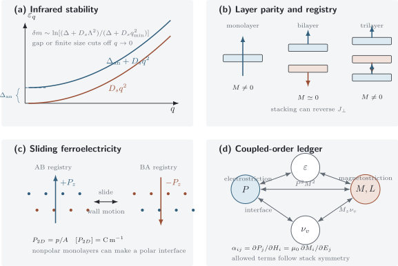
Four ledgers for atomically thin ferroic order. An anisotropy gap cuts off the infrared magnon divergence; antiferromagnetic interlayer exchange produces even–odd layer effects; lateral sliding interchanges opposite out-of-plane polar states; and symmetry determines which magnetic, electric, valley, and lattice responses can couple.

Anisotropy must be measured in the same device

Magnetic anisotropy can change with thickness because surface crystal fields, interlayer hybridization, strain, carrier density, and demagnetizing fields all change. A bulk easy axis cannot simply be assigned to a monolayer. Useful cross-checks include:

• angular dependence of saturation and spin-flop fields;
• zero-momentum magnon gaps from optical or microwave spectroscopy;
• domain-wall orientation and width;
• field-dependent transition temperatures;
• layer-resolved calculations tied to the measured structure.

The phrase “spin–orbit coupling stabilizes the magnet” is incomplete until it identifies the symmetry-allowed anisotropy and its scale relative to temperature and stiffness.

Layer-Dependent Magnetism

A stack is a coupled set of magnetic sheets

When each layer is internally ferromagnetic, a macrospin model isolates the interlayer ledger:

$$\begin{aligned} \frac{F}{A} ={}& J_\perp \sum_{\ell=1}^{N-1} \mathbf m_\ell\cdot\mathbf m_{\ell+1} \\ & -K_{2D}\sum_{\ell=1}^{N} (\mathbf m_\ell\cdot\hat{\mathbf z})^2 \\ &-\mu_0M_{2D} \mathbf H\cdot \sum_{\ell=1}^{N}\mathbf m_\ell . \end{aligned}$$

The unit vector $\mathbf m_\ell$ describes layer $\ell$; $J_\perp>0$ favors antiparallel neighboring layers in this convention; and $J_\perp$, $K_{2D}$, and $\mu_0M_{2D}H$ are energies per area. For collinear Ising layers, antiferromagnetic interlayer coupling gives a compensated even-layer stack and an uncompensated odd-layer stack.

For a bilayer in a perpendicular field, the ideal antiparallel and field-aligned energies are

$$\frac{F_{\mathrm{AF}}}{A}=-J_\perp, \qquad \frac{F_{\mathrm{F}}}{A} =J_\perp-2\mu_0M_{2D}H.$$

Their crossing occurs at

$$H_c = \frac{J_\perp}{\mu_0M_{2D}}.$$

This is a diagnostic baseline. Canting, anisotropy, domains, thermal fluctuations, unequal surface layers, and hysteresis modify the measured transition.

Layer number is not the only structural variable

Monolayer CrI$_3$ is an out-of-plane ferromagnet, while commonly studied bilayers exhibit layered antiferromagnetic coupling and a field-driven metamagnetic transition. Trilayers can recover a net moment. Yet interlayer exchange in CrI$_3$ is strongly stacking dependent: lateral registry, pressure, reconstruction, and twist can change its sign or create coexisting ferro- and antiferromagnetic regions. “Bilayer” is therefore insufficient metadata without stacking and structural history.

CrCl$_3$ provides a different limit with weak in-plane anisotropy and layer-parity-dependent spin-flop signatures. CrSBr combines ferromagnetic intralayer correlations with antiferromagnetic interlayer alignment, strong in-plane anisotropy, semiconducting transport, and excitons that sense the spin configuration. These systems show why one chemical family cannot stand in for all two-dimensional magnetism.

Gates can act through several channels

An applied gate can modify:

• carrier-mediated exchange and itinerant spin polarization;
• interlayer exchange through layer-selective doping;
• magnetic anisotropy through orbital occupation and interfacial electric fields;
• structural registry through electrostatic pressure or sliding;
• optical selection rules and the probe response itself.

The control variables should therefore be separated into carrier density $n$ and displacement field $D$. In a dual-gated device these are independent linear combinations of gate voltages only after the geometric and quantum capacitances are calibrated. A changed Kerr or tunnelling signal at fixed voltage is not automatically a changed magnetic ground state.

Ferroelectricity in van der Waals Systems

Polar, piezoelectric, and ferroelectric are different claims

A polar crystal has a symmetry-allowed spontaneous electric dipole. A piezoelectric crystal develops polarization under strain. A ferroelectric has at least two stable, symmetry-related polarization states that can be reversibly selected by an electric field. A pyroelectric response tracks a temperature-dependent spontaneous polarization. Ferroelectric implies polar, but polar and piezoelectric do not imply switchable ferroelectricity.

In an atomically thin system, the natural polarization is dipole moment per area,

$$\mathbf P_{2D} = \frac{\mathbf p}{A}, \qquad [\mathbf P_{2D}] =\mathrm{C\,m^{-1}}.$$

Reporting a three-dimensional value requires an assigned effective thickness,

$$\mathbf P_{3D} = \frac{\mathbf P_{2D}}{t_{\mathrm{eff}}}, \qquad [\mathbf P_{3D}] =\mathrm{C\,m^{-2}}.$$

The latter therefore depends on the thickness convention. For in-plane polarization, the bound line charge at an edge with outward normal $\hat{\mathbf n}$ is

$$\lambda_b = \mathbf P_{2D}\cdot\hat{\mathbf n}.$$

Polarization in a periodic quantum crystal is a Berry-phase quantity defined modulo a polarization quantum. Comparisons must use a continuous structural switching path, consistent unit cell, and the same branch. Berry-Phase Polarization and Charge Pumping owns that general branch and charge bookkeeping; this page retains the platform-specific switching, stability, and evidence audit for atomically thin ferroics.

Depolarization competes with the polar distortion

For a scalar out-of-plane sheet polarization $P$, a local Landau functional per area can be written

$$\begin{aligned} \frac{G}{A} ={}& \frac{a}{2}P^2 +\frac{b}{4}P^4 \\ &+\frac{\kappa_P}{2} \lvert\nabla P\rvert^2 -E_zP \\ &+\frac{G_{\mathrm{dep}}}{A}. \end{aligned}$$

with $b>0$. If $a<0$ and the depolarization term is controlled, the uniform minima are $P=\pm\sqrt{-a/b}$.

For an ideal open-circuit slab with three-dimensional polarization $P_{3D}$, thickness $t$, and background relative permittivity $\epsilon_b$, a simple unscreened estimate is

$$E_{\mathrm{dep}} \simeq -\frac{P_{3D}}{\epsilon_0\epsilon_b}, \qquad \frac{G_{\mathrm{dep}}}{A} \simeq \frac{tP_{3D}^2} {2\epsilon_0\epsilon_b}.$$

Electrodes, mobile carriers, adsorbates, substrates, and domain formation reduce or redistribute this cost. They can also create trapped-charge hysteresis that imitates switching, so screening is both a stabilizing mechanism and an experimental confounder.

Several microscopic routes exist

Route	Representative systems	Switching coordinate
intrinsic polar distortion	SnTe, CuInP$_2$S$_6$, $\alpha$-In$_2$Se$_3$	atomic displacement or order–disorder coordinate within a layer
polar few-layer stacking	few-layer WTe$_2$	relative registry of polar layers in a conducting stack
sliding ferroelectricity	parallel bilayer hBN, rhombohedral TMD bilayers	in-plane translation changes the sign of out-of-plane polarization
spin-driven polarity	NiI$_2$ and other candidate type-II multiferroics	noncollinear magnetic order breaks inversion and induces $P$

In sliding ferroelectrics, nonpolar monolayers can form a polar interface. AB and BA registries are related by a symmetry operation and carry opposite out-of-plane dipoles; an electric field moves domain walls or drives relative sliding. A small twist creates a moiré network of registries and polar domains rather than one uniform polarization.

Few-layer WTe$_2$ demonstrates that screening by itinerant carriers does not categorically forbid switchable polarity when the sample is thin enough for gates to penetrate. It does not imply that an arbitrary polar metal is ferroelectric.

An evidence ladder for ferroelectricity

Claim	Minimum evidence	Major confounder
noncentrosymmetric structure	diffraction, microscopy, or symmetry-resolved optics	surface sensitivity or an unidentified polytype
polar domains	calibrated electrostatic or structural contrast with reversed orientation	trapped charge, work-function patches, topography
electrically selected states	reproducible writing, retention, and opposite readout states	ionic motion, leakage, dielectric charging
ferroelectric switching	field-dependent domain-wall motion or polarization reversal tied to structure	PFM electrostatics and electrochemical strain
macroscopic polarization	switching current or charge integrated with leakage subtraction and geometry	capacitive transients and conductive paths

Piezoresponse force microscopy is valuable, but a phase contrast and butterfly loop are not sufficient alone. Frequency, humidity, contact force, off-field readout, retention, thickness, and flipped-sample controls help separate true electromechanical response from electrostatic and ionic artifacts.

Coupled Spin, Valley, and Lattice Orders

Symmetry comes before a coupling constant

Let $P$ be a polar order parameter, $\mathbf M$ a magnetization, $\mathbf L$ a Néel vector, $\varepsilon_{ij}$ strain, and $\nu_v=n_K-n_{K'}$ a valley polarization. A schematic uniform free energy may contain

$$\begin{aligned} \frac{G_{\mathrm{int}}}{A} ={}& \lambda_{PM}P^2\mathbf M^2 +\lambda_{PL}P^2\mathbf L^2 +q_{ij}P^2\varepsilon_{ij} \\ &+b_{ijkl}M_iM_j\varepsilon_{kl} +g_vM_z\nu_v +\cdots . \end{aligned}$$

Every displayed term is even under time reversal; whether it is allowed by spatial symmetry depends on the crystal, stack, and definition of the order parameters. If the high-symmetry parent has inversion, a term odd in $P$ is forbidden. Once a fixed polar interface already breaks inversion, lower-order couplings can become allowed.

For an electric- and magnetic-field thermodynamic potential,

$$dg = -P_j\,dE_j -\mu_0M_i\,dH_i,$$

the equilibrium linear magnetoelectric response obeys

$$\alpha_{ij} \equiv \frac{\partial P_j}{\partial H_i} = \mu_0 \frac{\partial M_i}{\partial E_j}.$$

Static linear magnetoelectricity is forbidden by either inversion or time reversal separately, although their product may remain a symmetry. Nonlinear, finite-frequency, interfacial, and nonequilibrium responses obey different selection rules.

Coexistence and coupling are different

In a type-I multiferroic, magnetic and polar orders have largely distinct microscopic origins; coupling can be useful without being strong. In a type-II multiferroic, magnetic order itself induces polarization. A common schematic bond contribution is

$$\mathbf P_{ij} \propto \hat{\mathbf e}_{ij} \times \left(\mathbf S_i\times\mathbf S_j\right),$$

but this inverse-Dzyaloshinskii–Moriya or spin-current form is not universal. Exchange striction, spin-dependent ligand hybridization, and other symmetry-allowed mechanisms can dominate.

NiI$_2$ is an important active example. Optical, nonlinear, electrical, and dynamical measurements support intertwined helical magnetic and polar order down to few-layer and reported monolayer limits, while calculations find close competition among spiral, striped, ferroic, and antiferroic states that depends on substrate, strain, and layer count. The durable conclusion is that it is a strong van der Waals multiferroic platform; the exact monolayer microscopic ground state remains structure sensitive.

Valleys can act as magnetic sensors

In a transition-metal dichalcogenide monolayer, time reversal exchanges the $K$ and $K'$ valleys. Exchange proximity to a magnet can therefore produce a valley-contrasting energy shift. In WSe$_2$/CrI$_3$ stacks, the exciton response can sense the magnetization of the interfacial CrI$_3$ layer and reveal layer-resolved magnetic transitions.

This is a coupled response, not necessarily spontaneous magnetism in the semiconductor. The observed optical splitting can also depend on spin-selective charge transfer, band alignment, exciton binding, and optical pumping. A calibrated magnetic probe and field-reversal symmetry are needed before translating an exciton shift into an “effective magnetic field.”

The lattice is an active participant

In atomically thin materials, strain and stacking alter bond angles, crystal fields, exchange paths, anisotropy, polarization, and valley energies at once. This makes twist, pressure, and domain walls unusually effective control variables, but it also creates causal ambiguity. A convincing control experiment should track the structural coordinate and show that the proposed magnetic or polar response follows it reversibly.

The most useful workflow is:

1. determine layer number, polytype, registry, twist, strain, and encapsulation;
2. identify the symmetries broken by each proposed order;
3. measure transition, domain, and excitation scales with complementary probes;
4. separate density from displacement field and temperature from Joule heating;
5. test reciprocity: electric control of magnetism and magnetic control of polarization;
6. compare with a model using the measured structure rather than an idealized bulk registry.

Common Mistakes

• Saying Mermin–Wagner forbids all two-dimensional magnetism. It addresses continuous symmetry and specified interaction assumptions in the thermodynamic limit.
• Calling every hysteresis loop ferromagnetic. Superparamagnetic blocking, pinning, contact effects, and sweep-rate dependence can also create loops.
• Using bulk anisotropy for a monolayer. Surface, strain, screening, and shape contributions change with thickness.
• Inferring interlayer order from net magnetization alone. Even–odd cancellation, domains, and unequal surface layers require layer-sensitive probes.
• Equating noncentrosymmetry with ferroelectricity. Switchable, stable, symmetry-related polar states must be demonstrated.
• Quoting a two-dimensional polarization in $\mathrm{C\,m^{-2}}$ without a thickness convention. The intrinsic sheet quantity has units $\mathrm{C\,m^{-1}}$.
• Treating PFM contrast as decisive proof. Electrostatics, ions, leakage, and topography need explicit controls.
• Calling coexistence magnetoelectric coupling. A coupling coefficient or reciprocal control must be measured.
• Calling an exchange-proximitized valley a spontaneous valley magnet. The symmetry breaking may reside entirely in the adjacent magnetic layer.
• Ignoring stacking history. Registry can reverse interlayer exchange or polarization without changing chemical composition.

Exercises

Exercise 1: infrared magnons

Starting from

$$I = \int_{q_{\min}}^\Lambda \frac{d^2q}{(2\pi)^2} \frac{k_BT} {\Delta+Dq^2},$$

evaluate $I$ and identify the two independent infrared cutoffs.

Solution

Using $d^2q=2\pi q\,dq$,

$$\begin{aligned} I &= \frac{k_BT}{2\pi} \int_{q_{\min}}^\Lambda \frac{q\,dq}{\Delta+Dq^2} \\ &= \frac{k_BT}{4\pi D} \ln \left( \frac{\Delta+D\Lambda^2} {\Delta+Dq_{\min}^2} \right). \end{aligned}$$

The anisotropy gap $\Delta$ and finite-size momentum $q_{\min}\sim2\pi/L$ are independent infrared cutoffs. If both vanish, the integral diverges logarithmically.

Exercise 2: finite size versus anisotropy

For a flake of size $L$, define an effective finite-size energy $\Delta_L=D(2\pi/L)^2$. Which cutoff controls the magnon integral when $\Delta\gg\Delta_L$ and when $\Delta\ll\Delta_L$? Does finite size establish a thermodynamic phase transition?

Solution

The denominator at the lowest mode is $\Delta+\Delta_L$. When $\Delta\gg\Delta_L$, anisotropy controls the infrared physics. When $\Delta\ll\Delta_L$, the finite lateral size controls it.

A finite flake can have a long correlation length and a stable moment over the measurement time, but it has no singular thermodynamic phase transition by itself. A transition is defined after a thermodynamic-limit or finite-size-scaling analysis.

Exercise 3: bilayer spin-flip field

Use the bilayer macrospin energies above to derive the field at which an antiparallel Ising bilayer becomes field aligned. What assumptions make this estimate fail?

Solution

Equating the two energies,

$$-J_\perp = J_\perp-2\mu_0M_{2D}H_c,$$

gives

$$\mu_0M_{2D}H_c = J_\perp.$$

The estimate assumes identical rigid layers, collinear Ising spins, zero temperature, a uniform single domain, and no hysteretic barrier. Canting, unequal moments, anisotropy, domains, thermal fluctuations, and stacking inhomogeneity shift or broaden the transition.

Exercise 4: sheet polarization

A monolayer has $P_{2D}=5.0\times10^{-13}\,\mathrm{C\,m^{-1}}$. Convert it to a three-dimensional polarization using $t_{\mathrm{eff}}=0.70\,\mathrm{nm}$. Repeat with $t_{\mathrm{eff}}=1.0\,\mathrm{nm}$ and explain the difference.

Solution

For $t_{\mathrm{eff}}=0.70\,\mathrm{nm}$,

$$\begin{aligned} P_{3D} &= \frac{5.0\times10^{-13}} {0.70\times10^{-9}} \\ &= 7.1\times10^{-4}\, \mathrm{C\,m^{-2}}. \end{aligned}$$

For $t_{\mathrm{eff}}=1.0\,\mathrm{nm}$,

$$P_{3D} = 5.0\times10^{-4}\,\mathrm{C\,m^{-2}}.$$

The physical sheet dipole is unchanged. The numerical three-dimensional value changes because the assigned thickness changes, which is why $P_{2D}$ is the intrinsic comparison for isolated layers.

Exercise 5: homogeneous ferroelectric spinodal

For

$$f(P) = \frac{a}{2}P^2 +\frac{b}{4}P^4 -EP,$$

with $a<0$ and $b>0$, find the field magnitude at which one homogeneous metastable minimum disappears.

Solution

At the spinodal, both derivatives vanish:

$$aP+bP^3-E=0, \qquad a+3bP^2=0.$$

Thus

$$P_{\mathrm{sp}}^2 = -\frac{a}{3b}.$$

Substitution gives the magnitude

$$\lvert E_{\mathrm{sp}}\rvert = \frac{2\lvert a\rvert^{3/2}} {3\sqrt{3b}}.$$

This is a homogeneous mean-field upper scale, not a realistic coercive field. Actual switching usually proceeds by nucleation and domain-wall motion at a smaller, geometry- and defect-dependent field.

Exercise 6: coupling shifts a magnetic transition

Consider

$$\begin{aligned} f ={}& \frac{a_P}{2}P^2 +\frac{b_P}{4}P^4 +\frac{a_M}{2}(T-T_{M0})M^2 \\ &+\frac{b_M}{4}M^4 +\frac{\lambda}{2}P^2M^2. \end{aligned}$$

Assume $P$ is already nonzero and varies slowly near the magnetic transition. Find the shifted mean-field magnetic transition temperature and interpret the sign of $\lambda$.

Solution

The quadratic coefficient of $M$ is

$$a_M(T-T_{M0}) +\lambda P^2.$$

It vanishes at

$$T_M = T_{M0} -\frac{\lambda P^2}{a_M}.$$

For $a_M>0$, positive $\lambda$ makes polarization and magnetization compete and lowers $T_M$; negative $\lambda$ makes them cooperate and raises $T_M$. This conclusion concerns a biquadratic equilibrium coupling. It does not by itself imply that reversing $P$ reverses $M$, because the term depends on $P^2$.

Research Status

Intrinsic monolayer and few-layer magnetic order is established in several insulating, semiconducting, and itinerant van der Waals families. The main open problems are no longer whether two-dimensional magnets can exist, but how disorder, stacking, itinerancy, finite size, and nonequilibrium probes determine their phase diagrams and switching kinetics.

Switchable polarization is established in several intrinsic and stacking-engineered two-dimensional systems. Quantitative comparison remains difficult because polarization units, effective thickness, electrodes, leakage, and local-probe artifacts differ between experiments. Sliding ferroelectricity has expanded the design space from polar compounds to interfaces assembled from nonpolar monolayers.

Coupled magnetism and ferroelectricity is more active. NiI$_2$ provides strong evidence for a van der Waals type-II multiferroic with large dynamical magnetoelectric response, but the precise monolayer state is sensitive to structure and remains under theoretical and experimental refinement. Across the field, reciprocal control, calibrated absolute response tensors, reproducible switching endurance, and direct structural tracking remain stronger tests than a single hysteretic optical or transport signal.

Summary

• Two-dimensional magnetic order survives when anisotropy, long-range interactions, interlayer coupling, or finite experimental scales change the assumptions of the isotropic thermodynamic-limit model.
• The magnon infrared integral shows directly why a small anisotropy gap can be decisive even when exchange sets the much larger stiffness.
• Layer number, parity, registry, twist, pressure, and gate configuration can change interlayer exchange and net magnetization.
• The intrinsic polarization of a layer is a sheet dipole density in $\mathrm{C\,m^{-1}}$; a bulk-like value requires an explicit thickness convention.
• Ferroelectricity requires stable, switchable polar states, not merely broken inversion, piezoresponse, or hysteresis.
• Sliding can create ferroelectricity at an interface even when each isolated monolayer is nonpolar.
• Coexisting magnetic and polar orders become multiferroically useful only when symmetry allows and experiment establishes a coupling or reciprocal response.
• Spin, valley, exciton, and lattice observables can probe one another, but the location of the broken symmetry must be identified.

Connections

• Low-Dimensional Quantum Matter develops dimensional crossover, infrared fluctuations, and finite-size caveats.
• Two-Dimensional Materials owns sheet structure, environmental screening, valleys, excitons, and device electrostatics.
• van der Waals Heterostructures develops assembly, interfaces, dual gates, proximity effects, tunnelling, and structural metrology.
• Engineered Heterostructures places magnetic proximity, ferroic control, and magnet–superconductor combinations inside a cross-platform interface evidence ladder.
• Moiré Superlattices owns twist-generated registry textures and emergent cells.
• Transition-Metal Dichalcogenides develops spin–valley locking and semiconductor heterostructures.
• Ferromagnetism and Antiferromagnetism supply the general order-parameter and excitation theory.
• Magnetic Anisotropy owns anisotropy tensors, easy axes and planes, shape effects, and switching fields.
• Spin–Orbit Coupling in Solids explains the microscopic bridge from crystal symmetry to spin anisotropy and valley locking.
• Spontaneous Symmetry Breaking gives the thermodynamic-limit language behind Mermin–Wagner constraints.

Further Reading

1. N. D. Mermin and H. Wagner, “Absence of Ferromagnetism or Antiferromagnetism in One- or Two-Dimensional Isotropic Heisenberg Models,” Physical Review Letters 17, 1133–1136 (1966), doi:10.1103/PhysRevLett.17.1133.
2. P. C. Hohenberg, “Existence of Long-Range Order in One and Two Dimensions,” Physical Review 158, 383–386 (1967), doi:10.1103/PhysRev.158.383.
3. J. M. Kosterlitz and D. J. Thouless, “Ordering, Metastability and Phase Transitions in Two-Dimensional Systems,” Journal of Physics C 6, 1181–1203 (1973), doi:10.1088/0022-3719/6/7/010.
4. B. Huang et al., “Layer-Dependent Ferromagnetism in a van der Waals Crystal down to the Monolayer Limit,” Nature 546, 270–273 (2017), doi:10.1038/nature22391.
5. C. Gong et al., “Discovery of Intrinsic Ferromagnetism in Two-Dimensional van der Waals Crystals,” Nature 546, 265–269 (2017), doi:10.1038/nature22060.
6. J.-U. Lee et al., “Ising-Type Magnetic Ordering in Atomically Thin FePS$_3$,” Nano Letters 16, 7433–7438 (2016), doi:10.1021/acs.nanolett.6b03052.
7. Y. Deng et al., “Gate-Tunable Room-Temperature Ferromagnetism in Two-Dimensional Fe$_3$GeTe$_2$,” Nature 563, 94–99 (2018), doi:10.1038/s41586-018-0626-9.
8. B. Huang et al., “Electrical Control of 2D Magnetism in Bilayer CrI$_3$,” Nature Nanotechnology 13, 544–548 (2018), doi:10.1038/s41565-018-0121-3.
9. S. Jiang et al., “Controlling Magnetism in 2D CrI$_3$ by Electrostatic Doping,” Nature Nanotechnology 13, 549–553 (2018), doi:10.1038/s41565-018-0135-x.
10. S. Jiang et al., “Electric-Field Switching of Two-Dimensional van der Waals Magnets,” Nature Materials 17, 406–410 (2018), doi:10.1038/s41563-018-0040-6.
11. T. Song et al., “Giant Tunneling Magnetoresistance in Spin-Filter van der Waals Heterostructures,” Science 360, 1214–1218 (2018), doi:10.1126/science.aar4851.
12. D. R. Klein et al., “Probing Magnetism in 2D van der Waals Crystalline Insulator CrI$_3$ with Graphene,” Science 360, 1218–1222 (2018), doi:10.1126/science.aar3617.
13. Z. Wang et al., “Determining the Phase Diagram of Atomically Thin Layered Antiferromagnet CrCl$_3$,” Nature Nanotechnology 14, 1116–1122 (2019), doi:10.1038/s41565-019-0565-0.
14. E. J. Telford et al., “Coupling between Magnetic Order and Charge Transport in a Two-Dimensional Magnetic Semiconductor,” Nature Materials 21, 754–760 (2022), doi:10.1038/s41563-022-01245-x.
15. Y. J. Bae et al., “Exciton-Coupled Coherent Magnons in a 2D Semiconductor,” Nature 609, 282–286 (2022), doi:10.1038/s41586-022-05024-1.
16. D. Zhong et al., “Layer-Resolved Magnetic Proximity Effect in van der Waals Heterostructures,” Nature Nanotechnology 15, 187–191 (2020), doi:10.1038/s41565-019-0629-1.
17. M. A. Tschudin et al., “Imaging Nanomagnetism and Magnetic Phase Transitions in Atomically Thin CrSBr,” Nature Communications 15, 6005 (2024), doi:10.1038/s41467-024-49717-9.
18. D. Soriano, M. I. Katsnelson, and J. Fernández-Rossier, “Magnetic Two-Dimensional Chromium Trihalides: A Theoretical Perspective,” Nano Letters 20, 6225–6234 (2020), doi:10.1021/acs.nanolett.0c02381.
19. J. L. Lado and J. Fernández-Rossier, “On the Origin of Magnetic Anisotropy in Two Dimensional CrI$_3$,” 2D Materials 4, 035002 (2017), doi:10.1088/2053-1583/aa75ed.
20. N. Sivadas et al., “Stacking-Dependent Magnetism in Bilayer CrI$_3$,” Nano Letters 18, 7658–7664 (2018), doi:10.1021/acs.nanolett.8b03321.
21. K. Chang et al., “Discovery of Robust In-Plane Ferroelectricity in Atomic-Thick SnTe,” Science 353, 274–278 (2016), doi:10.1126/science.aad8609.
22. F. Liu et al., “Room-Temperature Ferroelectricity in CuInP$_2$S$_6$ Ultrathin Flakes,” Nature Communications 7, 12357 (2016), doi:10.1038/ncomms12357.
23. Y. Zhou et al., “Out-of-Plane Piezoelectricity and Ferroelectricity in Layered $\alpha$-In$_2$Se$_3$ Nanoflakes,” Nano Letters 17, 5508–5513 (2017), doi:10.1021/acs.nanolett.7b02198.
24. J. Xiao et al., “Intrinsic Two-Dimensional Ferroelectricity with Dipole Locking,” Physical Review Letters 120, 227601 (2018), doi:10.1103/PhysRevLett.120.227601.
25. Z. Fei et al., “Ferroelectric Switching of a Two-Dimensional Metal,” Nature 560, 336–339 (2018), doi:10.1038/s41586-018-0336-3.
26. K. Yasuda et al., “Stacking-Engineered Ferroelectricity in Bilayer Boron Nitride,” Science 372, 1458–1462 (2021), doi:10.1126/science.abd3230.
27. M. Vizner Stern et al., “Interfacial Ferroelectricity by van der Waals Sliding,” Science 372, 1462–1466 (2021), doi:10.1126/science.abe8177.
28. X. Wang et al., “Interfacial Ferroelectricity in Rhombohedral-Stacked Bilayer Transition Metal Dichalcogenides,” Nature Nanotechnology 17, 367–371 (2022), doi:10.1038/s41565-021-01059-z.
29. A. Weston et al., “Interfacial Ferroelectricity in Marginally Twisted 2D Semiconductors,” Nature Nanotechnology 17, 390–395 (2022), doi:10.1038/s41565-022-01072-w.
30. R. D. King-Smith and D. Vanderbilt, “Theory of Polarization of Crystalline Solids,” Physical Review B 47, 1651–1654 (1993), doi:10.1103/PhysRevB.47.1651.
31. M. Dawber, K. M. Rabe, and J. F. Scott, “Physics of Thin-Film Ferroelectric Oxides,” Reviews of Modern Physics 77, 1083–1130 (2005), doi:10.1103/RevModPhys.77.1083.
32. Q. Song et al., “Evidence for a Single-Layer van der Waals Multiferroic,” Nature 602, 601–605 (2022), doi:10.1038/s41586-021-04337-x.
33. F. Y. Gao et al., “Giant Chiral Magnetoelectric Oscillations in a van der Waals Multiferroic,” Nature 632, 273–279 (2024), doi:10.1038/s41586-024-07678-5.
34. N. Liu et al., “Competing Multiferroic Phases in Monolayer and Few-Layer NiI$_2$,” Physical Review B 109, 195422 (2024), doi:10.1103/PhysRevB.109.195422.
35. Y. Wu et al., “Coexistence of Ferroelectricity and Antiferroelectricity in 2D van der Waals Multiferroic,” Nature Communications 15, 8616 (2024), doi:10.1038/s41467-024-53019-5.
36. H. Katsura, N. Nagaosa, and A. V. Balatsky, “Spin Current and Magnetoelectric Effect in Noncollinear Magnets,” Physical Review Letters 95, 057205 (2005), doi:10.1103/PhysRevLett.95.057205.
37. M. Mostovoy, “Ferroelectricity in Spiral Magnets,” Physical Review Letters 96, 067601 (2006), doi:10.1103/PhysRevLett.96.067601.
38. B. Huang et al., “Coexisting Ferromagnetic–Antiferromagnetic State in Twisted Bilayer CrI$_3$,” Nature Nanotechnology 17, 68–72 (2022), doi:10.1038/s41565-021-01014-y.
39. Z. Sun et al., “Giant Nonreciprocal Second-Harmonic Generation from Antiferromagnetic Bilayer CrI$_3$,” Nature 572, 497–501 (2019), doi:10.1038/s41586-019-1445-3.
40. M. Gibertini et al., “Magnetic 2D Materials and Heterostructures,” Nature Nanotechnology 14, 408–419 (2019), doi:10.1038/s41565-019-0438-6.