Moiré Superlattices

A moiré superlattice is a long-wavelength modulation produced when two or more periodic structures are combined with a small relative rotation, lattice mismatch, strain, or displacement texture. The atomic lattices supply rapidly varying phases; their differences produce a much longer geometric scale. Interlayer tunneling, local band-edge shifts, dielectric response, or lattice relaxation can then turn that geometric beat into a periodic quantum Hamiltonian.

Those statements form a hierarchy, not a chain of synonyms:

level	question	evidence
geometric moiré	do the layer phases form a long-period registry pattern?	calibrated atomic or reciprocal-space geometry
reconstructed lattice	how do atoms relax within the nominal pattern?	domains, strain, corrugation, and domain-wall maps
moiré Hamiltonian	which matrix elements vary with local registry?	continuum or atomistic model tied to measured structure
miniband system	do quantum states obey the emergent translation scale?	replicated bands, minigaps, filling closure, or magnetic commensurability
correlated moiré matter	do interactions reorganize the miniband states?	thermodynamic, spectroscopic, and transport evidence beyond a one-body model

A visible pattern establishes the first line. It does not, by itself, establish flat bands, a Hubbard model, or a correlated phase.

Canonical Scope

This page is the canonical home for the generic geometry and scale hierarchy of moiré quantum matter. It owns reciprocal-vector differences, moiré periods and unit-cell areas, mini Brillouin zones, continuum miniband construction, generic flattening mechanisms, interaction-versus-kinetic scaling, filling conversion, and the criteria for calling a solid an analog quantum simulator.

van der Waals Heterostructures owns assembly, alignment metrology, encapsulation, gates, contacts, proximity channels, and vertical tunneling. Graphene owns the engineered monolayer Dirac platform, while Transition-Metal Dichalcogenides owns spin–valley-locked semiconductor bands, interlayer excitons, and material-specific TMD moiré evidence.

Twisted Bilayer Graphene owns the Bistritzer–MacDonald model, magic-angle graphene phenomenology, correlated states, superconductivity, and valley topology. Flat Bands owns dispersionless-band mechanisms, compact localization, projector geometry, Chern-band constraints, and flat-band ferromagnetism across lattice systems. Correlated Insulators in Moiré Systems owns filling-controlled Mott-like, generalized Wigner, flavor-ordered, and topological insulating phases. Moiré Superconductivity owns phase-coherence criteria, pairing classifications, tunable superconducting regimes, and device evidence; Moiré Topology owns topological minibands and integer and fractional Hall phases across platforms. Reciprocal Lattice, Brillouin Zones, and Bloch’s Theorem retain the general crystal theory used here.

Geometric Origin of Moiré Patterns

Registry is a slowly varying field

Consider two nearly matched two-dimensional Bravais lattices. In a smooth description, their local relative displacement can be written

$$\begin{aligned} \mathbf d(\mathbf r) &= \left[ R(\theta)(I+\varepsilon)-I \right]\mathbf r + \mathbf d_0 \\ &\quad + \mathbf u_2(\mathbf r) - \mathbf u_1(\mathbf r). \end{aligned}$$

Here $R(\theta)$ is a relative rotation, $\varepsilon$ is heterostrain or lattice mismatch written as a deformation tensor, $\mathbf d_0$ fixes the global translation, and $\mathbf u_\ell$ are relaxation fields. Registry is defined modulo an atomic Bravais vector: adding such a vector to $\mathbf d$ describes the same local stacking.

Any registry-dependent scalar or matrix $F(\mathbf d)$ is periodic on that atomic displacement space. Its Fourier expansion is

$$F\!\left(\mathbf d(\mathbf r)\right) = \sum_{\mathbf G} F_{\mathbf G} e^{i\mathbf G\cdot\mathbf d(\mathbf r)}.$$

For a rigid deformation, the phase varies with an emergent wavevector

$$\mathbf g_{\mathbf G} = \left[ R(\theta)(I+\varepsilon)-I \right]^{T} \mathbf G.$$

Small rotation or mismatch makes $|\mathbf g_{\mathbf G}|\ll|\mathbf G|$, so the corresponding real-space modulation is much longer than the atomic period. This is the two-dimensional version of beating between nearby frequencies.

Reciprocal differences define the emergent lattice

Choose paired reciprocal bases $\mathbf b_i^{(1)}$ and $\mathbf b_i^{(2)}$ for the two layers. A convenient moiré reciprocal basis is

$$\mathbf g_i = \mathbf b_i^{(1)} - \mathbf b_i^{(2)}.$$

The associated direct basis $\mathbf A_i$ is defined by

$$\mathbf A_i\cdot\mathbf g_j = 2\pi\delta_{ij}.$$

This construction is basis-independent up to integer changes of primitive vectors, but sign conventions differ across the literature. A calculation should state which layer is rotated, how positive twist is defined, and which reciprocal vectors are paired. Those choices change labels and orientations, not measurable spectra.

Exact periodicity is not automatic

Only special relative rotations and lattice ratios produce an exact common atomic supercell. A generic twisted bilayer is incommensurate: no finite translation maps every atom in both layers onto an equivalent atom. Nevertheless, smooth registry-dependent terms can be extremely well represented by a periodic continuum model over a moiré cell.

That approximation must be named. Three descriptions are common:

1. an exact commensurate supercell at a permitted angle;
2. a nearby commensurate approximant to an incommensurate structure;
3. a continuum model periodic in the slow registry coordinate.

They need not agree when atomic relaxation, quasiperiodicity, disorder, or boundaries matter on the target scale.

Moiré Length Scale

Twist and mismatch enter together

For identical triangular lattices with lattice constant $a$ and relative twist $\theta$, the rigid moiré period is

$$L_M = \frac{a} {2\sin\!\left(|\theta|/2\right)} \simeq \frac{a}{|\theta|}, \qquad |\theta|\ll1,$$

where the small-angle expression requires $\theta$ in radians.

Now let $a_1=a$ and $a_2=(1+\delta)a$. For isotropic mismatch $\delta$ and relative twist $\theta$, the shortest reciprocal mismatch and the corresponding triangular moiré period are

$$\begin{aligned} g_M &= \frac{4\pi}{\sqrt3\,a} \frac{ \sqrt{ \delta^2 + 4(1+\delta)\sin^2(\theta/2) } }{1+\delta}, \\ L_M &= \frac{4\pi}{\sqrt3\,g_M} \\ &= \frac{ a(1+\delta) }{ \sqrt{ \delta^2 + 4(1+\delta)\sin^2(\theta/2) } }. \end{aligned}$$

When $|\delta|,|\theta|\ll1$,

$$L_M \simeq \frac{a} {\sqrt{\delta^2+\theta^2}}.$$

Twist and mismatch therefore do not define independent long periods in this isotropic limit; they combine as orthogonal components of the reciprocal mismatch. Heterostrain is tensorial and generally makes the three shortest moiré vectors unequal, distorting a hexagonal cell into an oblique one.

Cell area converts density into filling

For a triangular moiré lattice,

$$A_M = \frac{\sqrt3}{2}L_M^2, \qquad n_M = \frac{1}{A_M}.$$

If $\nu$ denotes carriers per moiré cell relative to a stated reference,

$$n-n_{\mathrm{ref}} = \frac{\nu}{A_M}.$$

The conversion is purely geometric. Spin, valley, layer, and orbital degeneracies determine how many carriers fill a chosen miniband manifold, but they do not alter $n_M$. Authors use incompatible $\nu$ origins and signs, so a filling label is incomplete unless the reference state and degeneracy are specified.

For identical graphene lattices with $a=0.246\,\mathrm{nm}$ and $\theta=1.10^\circ$,

$$\begin{aligned} L_M &\simeq 12.8\,\mathrm{nm}, \\ A_M &\simeq 142\,\mathrm{nm}^2, \\ n_M &\simeq 7.0\times10^{11}\,\mathrm{cm}^{-2}. \end{aligned}$$

A fourfold manifold therefore changes occupancy by four carriers per cell over a density interval near $2.8\times10^{12}\,\mathrm{cm}^{-2}$. The numerical value is a geometry check, not proof that the fourfold manifold is isolated or symmetry-degenerate.

Angle uncertainty grows at small twist

For a twist-dominated pattern, $L_M\propto1/|\theta|$, so

$$\frac{\Delta L_M}{L_M} \simeq \frac{\Delta\theta}{|\theta|}.$$

An absolute angular uncertainty that looks small can therefore produce a substantial spread in cell area, filling density, and bandwidth. Local heterostrain and twist gradients add spatial variation. Reporting one nominal angle without a distribution can conceal the dominant uncertainty in a phase diagram.

Relaxation reconstructs the rigid pattern

The rigid geometry supplies a registry field, not the final atomic structure. A schematic elastic-adhesion functional is

$$\begin{aligned} E[\mathbf u] &= \int d^2r \left[ \mathcal E_{\mathrm{el}}(\mathbf r) + V_{\mathrm{stack}}\!\left(\mathbf d(\mathbf r)\right) \right], \\ \mathcal E_{\mathrm{el}}(\mathbf r) &= \frac12 C_{ijkl} \epsilon_{ij}(\mathbf r) \epsilon_{kl}(\mathbf r). \end{aligned}$$

Elasticity penalizes rapid deformation, while the stacking energy favors selected registries. At sufficiently long moiré periods, the compromise can enlarge low-energy domains and concentrate mismatch into narrow soliton-like walls. Out-of-plane corrugation may accompany in-plane reconstruction. The electronic potential must then be built from the relaxed registry map, not merely from two rigid lattices.

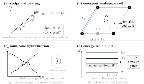
The moiré hierarchy. (a) Nearby reciprocal vectors differ by a small $\mathbf g_M$, producing a long beat scale. (b) The emergent cell contains distinct local registries and may reconstruct into domains and walls. (c) Folding into the mini Brillouin zone creates crossings; coupling opens minigaps and reshapes the minibands. (d) Correlated behavior depends on the measured ordering of bandwidth $W$, isolation gaps $\Delta_\pm$, Coulomb scale $E_C$, disorder broadening $\Gamma$, and $k_BT$.

Mini Brillouin Zones

The moiré cell has its own reciprocal fundamental domain

Once a periodic moiré Hamiltonian is justified, the reciprocal vectors

$$\mathbf G_M = m_1\mathbf g_1 + m_2\mathbf g_2, \qquad m_i\in\mathbb Z,$$

define a moiré reciprocal lattice. Its first Brillouin zone has area

$$\mathcal A_{\mathrm{mBZ}} = \frac{(2\pi)^2}{A_M}.$$

The mini Brillouin zone is not an additional set of states. It is the reduced-zone bookkeeping appropriate to the enlarged real-space cell. Atomic-layer momenta separated by a moiré reciprocal vector are represented at the same mini-zone momentum and can hybridize when the Hamiltonian supplies the corresponding Fourier component.

Continuum Hamiltonians retain the slow couplings

A generic bilayer continuum model has the block form

$$\begin{gathered} \mathcal H(\mathbf r) = \begin{pmatrix} \widetilde h_1(\mathbf r) & T(\mathbf r) \\ T^\dagger(\mathbf r) & \widetilde h_2(\mathbf r) \end{pmatrix}, \\ \widetilde h_\ell(\mathbf r) = h_\ell(-i\boldsymbol\nabla) + V_\ell(\mathbf r). \end{gathered}$$

with

$$\begin{aligned} V_\ell(\mathbf r+\mathbf A_i) &= V_\ell(\mathbf r), \\ T(\mathbf r+\mathbf A_i) &= T(\mathbf r). \end{aligned}$$

$h_\ell$ describes the isolated-layer bands in a chosen valley and orbital basis. $V_\ell$ contains registry-dependent intralayer terms, and $T$ contains interlayer tunneling. Their matrix structure can act on sublattice, orbital, spin, valley, layer, and Nambu indices. A scalar sinusoidal potential is only one special case.

Expand the slow terms as

$$T(\mathbf r) = \sum_{\mathbf G_M} T_{\mathbf G_M} e^{i\mathbf G_M\cdot\mathbf r},$$

and similarly for $V_\ell$. Bloch states of the continuum model obey

$$\Psi_{n\mathbf k}(\mathbf r) = e^{i\mathbf k\cdot\mathbf r} u_{n\mathbf k}(\mathbf r), \qquad \mathbf k\in\mathrm{mBZ},$$

where $u_{n\mathbf k}$ is moiré-periodic. In a plane-wave calculation, its components carry momenta $\mathbf k+\mathbf G_M$. Truncating that reciprocal set is a numerical approximation whose convergence must be checked for energies, wavefunctions, symmetry eigenvalues, and Berry quantities.

Folding is not flattening

If the layer coupling were set to zero, writing the original dispersions in the mini zone would merely fold them into many branches. Fourier components of $V_\ell$ and $T$ then open avoided crossings, exchange layer and orbital character, and can isolate groups of bands. The relevant local two-level structure is

$$\mathcal H_{\mathrm{cross}} = \begin{pmatrix} \epsilon_1(\mathbf k) & t_{\mathbf g} \\ t_{\mathbf g}^{*} & \epsilon_2(\mathbf k+\mathbf g) \end{pmatrix}.$$

At degeneracy, the direct minigap is $2|t_{\mathbf g}|$. Away from degeneracy, hybridization falls with detuning. Observing a replica band without a controlled anticrossing can reflect matrix elements, final-state diffraction, domains, or an analysis convention rather than a coherent miniband.

Use a model hierarchy

description	resolves well	principal audit
atomistic first-principles or tight binding	local chemistry, relaxation, orbital-scale tunneling	supercell or approximant size, parametrization, computational convergence
continuum model	long-wavelength coupling, arbitrary small angle, symmetry, minibands	basis choice, retained harmonics, relaxation input, momentum cutoff
Wannier or lattice model	interactions, ordered phases, scalable many-body methods	band isolation, gauge choice, topology, interaction range

Agreement at one band edge does not validate the whole hierarchy. A controlled reduction should reproduce the target dispersion, wavefunction character, symmetries, and response over a stated energy and parameter window.

Flat Minibands

Flatness requires a scale comparison

For an isolated band $n$, define

$$W_n = \max_{\mathbf k}E_{n\mathbf k} - \min_{\mathbf k}E_{n\mathbf k}.$$

Global gaps to adjacent bands may be defined as

$$\begin{aligned} \Delta_+ &= \min_{\mathbf k}E_{n+1,\mathbf k} - \max_{\mathbf k}E_{n,\mathbf k}, \\ \Delta_- &= \min_{\mathbf k}E_{n,\mathbf k} - \max_{\mathbf k}E_{n-1,\mathbf k}. \end{aligned}$$

Positive $\Delta_\pm$ establish energetic isolation. A ratio such as

$$\mathcal F = \frac{\min(\Delta_+,\Delta_-)}{W_n}$$

is a useful flatness indicator, but it is not universal. For a connected multiband manifold, $W$ and the remote-band gaps must be defined for the whole manifold. Disorder broadening $\Gamma$, thermal energy $k_BT$, interaction scales, and measurement resolution also belong in the comparison.

Several mechanisms narrow moiré bands

1. Large-cell kinetic suppression. A long period reduces the momentum scale over which a miniband disperses.
2. Hybridization interference. Coupling among momentum-space copies can cancel velocities or hopping amplitudes at special parameters.
3. Registry localization. A deep moiré potential can trap wavefunctions near selected stackings, making intercell tunneling exponentially small.
4. Structural reconstruction. Domains, corrugation, and walls reshape both onsite energies and tunneling networks.
5. Symmetry and band geometry. Protected crossings, fragile connectivity, Berry curvature, and topology can constrain whether a narrow manifold admits simple localized orbitals.

Zone folding alone does not reduce the physical velocity of an uncoupled band. Conversely, a band can have a small total width yet remain unsuitable for a one-orbital model because it overlaps remote bands or carries a Wannier obstruction.

Kinetic scales depend on the parent dispersion

For a parabolic band with effective mass $m^*$, a geometric kinetic estimate is

$$E_M^{\mathrm{par}} \sim \frac{\hbar^2}{2m^*L_M^2}.$$

For a Dirac cone with velocity $v$,

$$E_M^{\mathrm{Dirac}} \sim \frac{\hbar v}{L_M}.$$

These estimates give the scale before detailed hybridization. They explain why increasing $L_M$ suppresses parabolic kinetic energy faster than the bare Coulomb scale. In a Dirac system, strong flattening generally requires more than a large unit cell: interlayer interference and velocity renormalization are central.

Tunable Interactions

Coulomb and kinetic scales transform differently

A rough unscreened interaction scale across one moiré cell is

$$E_C \sim \frac{e^2} {4\pi\epsilon_0\epsilon_{\mathrm{eff}}L_M}.$$

Combining this with the parabolic estimate gives

$$\frac{E_C}{E_M^{\mathrm{par}}} \sim \frac{2L_M}{a_B^*}, \qquad a_B^* = \frac{ 4\pi\epsilon_0\epsilon_{\mathrm{eff}}\hbar^2 }{ m^*e^2 }.$$

Thus a longer moiré period can parametrically strengthen interactions relative to parabolic kinetic energy. For an unrenormalized Dirac cone,

$$\frac{E_C}{E_M^{\mathrm{Dirac}}} \sim \frac{e^2} {4\pi\epsilon_0\epsilon_{\mathrm{eff}}\hbar v},$$

which is independent of $L_M$ at this level. Moiré hybridization can nevertheless reduce the operative velocity or bandwidth and thereby enhance correlations.

These are scaling estimates, not Hubbard parameters. The actual matrix elements depend on wavefunction extent, layer polarization, dielectric nonlocality, metallic gates, form factors, and remote-band screening.

Gates reshape the interaction, not just the density

For a two-dimensional charge layer centered between metallic gates a distance $d$ above and below, a representative Fourier-space interaction is

$$V(q) = \frac{e^2} {2\epsilon_0\epsilon_{\mathrm{eff}}q} \tanh(qd).$$

At $qd\gg1$, the gates are ineffective at that wavelength. At $qd\ll1$, long-range components are strongly reduced. Real stacks can have unequal gate distances, anisotropic dielectrics, multiple conducting layers, and density-dependent internal screening, so the electrostatic geometry belongs in every quoted interaction parameter.

Projection produces an extended model

Projecting isolated minibands into localized orbitals gives a schematic Hamiltonian

$$\begin{aligned} H_{\mathrm{eff}} &= H_t+H_V+H_{\mathrm{res}}, \\ H_t &= \sum_{ij,ab} t_{ij}^{ab} c_{ia}^{\dagger}c_{jb} \\ H_V &= \frac12 \sum_{ij,ab} V_{ij}^{ab} n_{ia}n_{jb} , \\ H_{\mathrm{res}} &= H_{\mathrm{exchange}} + H_{\mathrm{pair}} + \cdots . \end{aligned}$$

The labels $a,b$ may encode spin, valley, layer, orbital, or sublattice. Long moiré orbitals often make intersite repulsion appreciable; intervalley exchange, assisted hopping, phonons, and remote bands can also matter. If the active manifold is topological or symmetry-obstructed, a single localized orbital per apparent potential minimum may not exist without adding bands or sacrificing a symmetry.

Hubbard Physics in Materials owns the full model-to-material validation workflow. A moiré pattern makes Hubbard-family descriptions tunable; it does not make a nearest-neighbor Hubbard model automatic.

Control parameters have coupled consequences

control	intended effect	coupled consequence
twist or lattice mismatch	period, symmetry, bandwidth	angle disorder, reconstruction, changed orbital overlap
displacement field	layer polarization and band offsets	topology, screening, contact density
pressure or interlayer spacing	stronger hybridization	relaxation, strain, possible hysteresis
carrier density	filling and Fermi level	screening, Hartree reconstruction, flavor polarization
dielectric and gate distance	interaction range and strength	disorder environment, phonons, capacitance
heterostrain	anisotropy and bandwidth	spatially varying period and broken symmetry
magnetic field	flux per cell and flavor splitting	orbital quantization, Zeeman energy, contact response

Twist is usually a fabrication parameter rather than an in situ knob. Mechanically rotatable devices are an important exception, but they introduce their own friction, relaxation, and metrology requirements.

Why Moiré Systems Are Quantum Simulators in Solids

The claim is about a validated parameter map

An analog quantum simulator realizes a target Hamiltonian well enough that controlled changes of physical inputs map to known changes of model parameters and measured observables test the model’s predictions. In moiré matter, the simulator degrees of freedom are real electrons, holes, or excitons inside a solid. The platform is tunable, but it is not a universal digital quantum computer and is not automatically programmable term by term.

Moiré systems are attractive because geometry can create large, accessible unit cells; gates tune filling without chemical substitution; displacement fields and pressure reshape wavefunctions; and transport, capacitance, optics, tunneling, and local probes interrogate complementary observables. Different registry patterns can produce triangular, honeycomb, rectangular, or multiorbital effective lattices.

target structure	possible moiré realization	term that must be checked
triangular fermion lattice	one dominant semiconductor registry minimum per cell	long-range repulsion and spin–valley structure
honeycomb lattice	two symmetry-related active registries	sublattice imbalance and further-neighbor hopping
layer or orbital pseudospin model	two active layers or miniband orbitals	interlayer tunneling and capacitive coupling
bosonic lattice	trapped interlayer excitons	lifetime, dipolar interaction, and nonequilibrium population
topological lattice band	miniband Berry curvature and band inversion	remote-band mixing and interaction-driven reconstruction

The analogy to Optical Lattices is useful but limited. Cold-atom platforms offer clean microscopic control and direct time-domain protocols; solids offer high particle density, electronic energy scales, natural long-range Coulomb interactions, and mature electrical and spectroscopic probes. Moiré devices also inherit disorder, strain, contacts, phonons, dielectric uncertainty, and limited microscopic programmability.

Simulator validation has an evidence ladder

1. Close the geometry. Measure local period, orientation, heterostrain, domains, and uncertainty rather than quoting only a fabrication angle.
2. Establish the active manifold. Identify miniband width, remote-band gaps, degeneracies, layer and orbital character, and spatial variation.
3. Calibrate filling. Reconcile gate capacitance, quantum capacitance, Hall density, and the density interval per moiré cell.
4. Derive the model. Document Wannier or continuum basis, hopping, interaction matrix elements, screening, and omitted terms.
5. Predict several observables. Use the same parameters for thermodynamics, spectroscopy, transport, and symmetry response where possible.
6. Test tunability. Verify that pressure, field, density, or displacement changes the inferred parameters in the predicted direction and magnitude.
7. Bound alternatives. Exclude disorder localization, percolation, contacts, heating, structural transitions, and flavor-dependent parallel channels.

A successful fit to one resistance curve is model compatibility, not model validation.

Experimental Diagnostics

claim	primary diagnostic	necessary cross-check
moiré period and symmetry	STM, TEM, diffraction, or calibrated real-space imaging	local angle and strain distribution
miniband formation	ARPES, tunneling spectra, optical transitions, or transport satellites	filling periodicity and coupling-dependent anticrossings
isolated narrow manifold	bandwidth plus upper and lower gaps	disorder and temperature broadening
integer filling	capacitance or density calibration	Hall response and cell-area consistency
interaction-driven incompressibility	chemical-potential jump or compressibility minimum	one-body gap calculation and disorder control
magnetic-flux commensurability	features versus $\Phi/\Phi_0=BA_M/\Phi_0$	independently measured $A_M$ and field calibration

The large moiré area makes one flux quantum per cell reachable at laboratory magnetic fields:

$$B_{\Phi_0} = \frac{\Phi_0}{A_M}, \qquad \Phi_0 = \frac{h}{e}.$$

This enables magnetic minibands and Hofstadter-type spectra. Magnetic Translations owns the underlying projective translation algebra.

Common Mistakes

Treating every interference image as an exact crystal

A long-period contrast can exist in an incommensurate or spatially varying stack. State whether the theory uses an exact supercell, an approximant, or a continuum registry model.

Using degrees in a small-angle formula

$L_M\simeq a/|\theta|$ requires radians. Using degrees underestimates the period by a factor of about $57.3$.

Inferring electronic flatness from a long period

A large unit cell reduces characteristic kinetic scales but does not guarantee velocity cancellation, localization, remote-band isolation, or a small measured bandwidth.

Calling a folded plot a miniband measurement

Reduced-zone plotting creates replicas even without coupling. Coherent reconstruction requires minigaps, exchanged character, filling closure, or another coupling-sensitive signature.

Equating integer carriers per cell with a Mott state

Band gaps, flavor polarization, charge order, disorder, and percolation can all produce insulating transport at commensurate filling. Thermodynamic and spectroscopic evidence must identify the mechanism.

Quoting one Hubbard interaction

Moiré orbitals are extended, screening is nonlocal, and neighboring-cell repulsion may be comparable to onsite terms. Report the orbital basis, interaction tensor, gate geometry, and truncation.

Ignoring reconstruction and inhomogeneity

The rigid moiré period is a starting geometry. Domains, walls, bubbles, heterostrain, and twist gradients can dominate spectra and transport.

Exercises

Exercise 1: twist period and angular sensitivity

Two identical hexagonal layers have $a=0.330\,\mathrm{nm}$ and twist angle $\theta=1.50^\circ\pm0.05^\circ$. Find the rigid moiré period and its leading uncertainty.

Solution

Convert the angle to radians:

$$\theta = 1.50\frac{\pi}{180} \simeq 0.02618.$$

The exact period is

$$\begin{aligned} L_M &= \frac{0.330\,\mathrm{nm}} {2\sin(0.75^\circ)} \\ &\simeq 12.6\,\mathrm{nm}. \end{aligned}$$

For a twist-dominated pattern,

$$\frac{\Delta L_M}{L_M} \simeq \frac{0.05}{1.50} = 0.0333.$$

Thus

$$\Delta L_M \simeq 0.42\,\mathrm{nm},$$

so the result is $L_M\simeq(12.6\pm0.4)\,\mathrm{nm}$. This uncertainty excludes local twist gradients and heterostrain.

Exercise 2: twist and mismatch

Two triangular lattices have $a=0.330\,\mathrm{nm}$, isotropic mismatch $\delta=0.040$, and twist $\theta=1.0^\circ$. Estimate $L_M$ using the small-parameter formula. Which contribution dominates?

Solution

In radians, $\theta\simeq0.01745$. Therefore

$$\begin{aligned} L_M &\simeq \frac{0.330\,\mathrm{nm}} {\sqrt{0.040^2+0.01745^2}} \\ &\simeq 7.56\,\mathrm{nm}. \end{aligned}$$

Because $\delta^2=1.60\times10^{-3}$ while $\theta^2\simeq3.05\times10^{-4}$, mismatch supplies about $84\%$ of the squared reciprocal offset. Calling this a twist-controlled period would therefore be misleading.

Exercise 3: density per moiré cell

A triangular moiré lattice has $L_M=10.0\,\mathrm{nm}$. Compute the density change corresponding to one carrier per cell and to four carriers per cell.

Solution

The cell area is

$$A_M = \frac{\sqrt3}{2} (10.0\,\mathrm{nm})^2 \simeq 86.6\,\mathrm{nm}^2.$$

Since $1\,\mathrm{nm}^{-2}=10^{14}\,\mathrm{cm}^{-2}$,

$$\begin{aligned} n_M &= \frac{1}{A_M} \simeq 1.15\times10^{12}\,\mathrm{cm}^{-2}, \\ 4n_M &\simeq 4.62\times10^{12}\,\mathrm{cm}^{-2}. \end{aligned}$$

The second number is the density span of a four-state-per-cell manifold only if those four states form the active isolated manifold.

Exercise 4: kinetic and Coulomb estimates

Take a parabolic moiré band with $m^*=0.50m_e$, $L_M=8.0\,\mathrm{nm}$, and $\epsilon_{\mathrm{eff}}=10$. Estimate $E_M^{\mathrm{par}}$, $E_C$, and their ratio using $\hbar^2/(2m_e)=0.0381\,\mathrm{eV\,nm^2}$ and $e^2/(4\pi\epsilon_0)=1.44\,\mathrm{eV\,nm}$.

Solution

The kinetic estimate is

$$\begin{aligned} E_M^{\mathrm{par}} &= \frac{0.0381\,\mathrm{eV\,nm^2}} {(0.50)(8.0\,\mathrm{nm})^2} \\ &\simeq 1.19\,\mathrm{meV}. \end{aligned}$$

The Coulomb estimate is

$$\begin{aligned} E_C &= \frac{1.44\,\mathrm{eV\,nm}} {(10)(8.0\,\mathrm{nm})} \\ &= 18.0\,\mathrm{meV}. \end{aligned}$$

Hence $E_C/E_M^{\mathrm{par}}\simeq15$. This signals a potentially interaction-dominated regime, but it is not a prediction of an onsite $U=18\,\mathrm{meV}$: gates, orbital form factors, intersite terms, and internal screening still have to be included.

Exercise 5: gate screening at a moiré wavevector

For symmetric metallic gates at $d=5.0\,\mathrm{nm}$, compare the interaction factor $\tanh(qd)$ at $q=1/L_M$ for $L_M=10\,\mathrm{nm}$ with the ungated value.

Solution

Here

$$qd = \frac{d}{L_M} = 0.50.$$

Therefore

$$\tanh(qd) = \tanh(0.50) \simeq 0.462.$$

At this representative wavevector, the symmetric gates reduce the bare Fourier-space interaction to about $46\%$ of its ungated value. Components with smaller $q$ are suppressed more strongly, while short-wavelength components with $qd\gg1$ are nearly unchanged.

Exercise 6: audit a correlated-insulator claim

A device shows a resistance peak at the gate voltage assigned to one carrier per moiré cell. List six checks needed before calling the state a moiré Mott insulator.

Solution

A defensible audit should include at least:

1. local measurements of moiré area, twist variation, heterostrain, and reconstruction;
2. a density calibration that reconciles geometric capacitance, quantum capacitance, offsets, and Hall response;
3. evidence that the active miniband is isolated and its degeneracy is known;
4. thermodynamic incompressibility or a chemical-potential jump, not resistance alone;
5. comparison with one-body band gaps, flavor polarization, charge order, disorder localization, and percolation;
6. temperature, field, displacement, pressure, and device-to-device trends tested against one parameterized effective model.

Spectroscopy of spectral-weight transfer or local charge order would further distinguish mechanisms. Integer filling is a location in parameter space, not a diagnosis.

Summary

• Nearby reciprocal vectors generate a long moiré scale; exact atomic commensurability is a separate question.
• For identical lattices, $L_M=a/[2\sin(|\theta|/2)]$; small mismatch and twist combine as $L_M\simeq a/\sqrt{\delta^2+\theta^2}$.
• The unit-cell area converts carrier density to filling, but degeneracy and the filling reference must be stated separately.
• A mini Brillouin zone becomes physically consequential when registry-dependent tunneling or potentials hybridize folded states and open minigaps.
• Narrow bandwidth, remote-band isolation, interaction strength, disorder, and temperature are distinct scales.
• Moiré projection generally produces an extended multicomponent model, not automatically a one-band onsite Hubbard model.
• Calling a moiré solid a quantum simulator requires a calibrated map from structure and controls to Hamiltonian parameters and multiple observables.

Connections

• Quantum Matter Frontiers and Open Problems audits a fast-moving moiré or flat-band claim across preparation, filling, projector geometry, alternatives, replication, and review triggers without turning this stable geometry-and-scale owner into a living status tracker.
• van der Waals Heterostructures develops the stack-level assembly, alignment, gate, contact, proximity, and tunneling ledger.
• Graphene supplies the engineered Dirac starting point for graphene superlattices.
• Twisted Bilayer Graphene applies this generic construction to the continuum model, first magic regime, correlated phases, superconductivity, and valley topology of TBG.
• Flat Bands separates exact and approximate flatness, compact localized states, quantum geometry, Chern bands, and rigorous ferromagnetism conditions.
• Correlated Insulators in Moiré Systems develops the evidence hierarchy from calibrated commensurability to thermodynamic gaps, charge order, flavor order, and model validation.
• Moiré Superconductivity applies the same calibration discipline to pairing, phase stiffness, BKT coherence, microscopic mechanisms, and gate-defined Josephson probes.
• Moiré Topology follows miniband isolation and flavor structure into Chern, quantum anomalous Hall, and fractional Chern phases.
• Transition-Metal Dichalcogenides develops semiconductor valleys, excitons, and TMD-specific correlated moiré evidence.
• Reciprocal Lattice and Brillouin Zones own the general direct-reciprocal duality and reduced-zone construction.
• Wannier Functions owns the Bloch-projector-to-localized-basis construction, localization, and obstruction tests; Tight-Binding Models owns hopping conventions and validation of the resulting model.
• Hubbard Physics in Materials gives the canonical active-space, interaction, solver, and validation workflow.
• Mott Insulators distinguishes interaction-driven incompressibility from transport-only and one-body alternatives.
• Optical Lattices provides a complementary analog-simulation platform with different controls and error sources.
• Magnetic Translations explains flux-dependent translation algebra and the origin of Hofstadter magnetic subbands.

Further Reading

1. J. M. B. Lopes dos Santos, N. M. R. Peres, and A. H. Castro Neto, “Graphene Bilayer with a Twist: Electronic Structure,” Physical Review Letters 99, 256802 (2007), doi:10.1103/PhysRevLett.99.256802.
2. R. Bistritzer and A. H. MacDonald, “Moiré Bands in Twisted Double-Layer Graphene,” Proceedings of the National Academy of Sciences 108, 12233–12237 (2011), doi:10.1073/pnas.1108174108.
3. M. Yankowitz et al., “Emergence of Superlattice Dirac Points in Graphene on Hexagonal Boron Nitride,” Nature Physics 8, 382–386 (2012), doi:10.1038/nphys2272.
4. L. A. Ponomarenko et al., “Cloning of Dirac Fermions in Graphene Superlattices,” Nature 497, 594–597 (2013), doi:10.1038/nature12187.
5. C. R. Dean et al., “Hofstadter’s Butterfly and the Fractal Quantum Hall Effect in Moiré Superlattices,” Nature 497, 598–602 (2013), doi:10.1038/nature12186.
6. B. Hunt et al., “Massive Dirac Fermions and Hofstadter Butterfly in a van der Waals Heterostructure,” Science 340, 1427–1430 (2013), doi:10.1126/science.1237240.
7. C. R. Woods et al., “Commensurate–Incommensurate Transition in Graphene on Hexagonal Boron Nitride,” Nature Physics 10, 451–456 (2014), doi:10.1038/nphys2954.
8. K. Kim et al., “Tunable Moiré Bands and Strong Correlations in Small-Twist-Angle Bilayer Graphene,” Proceedings of the National Academy of Sciences 114, 3364–3369 (2017), doi:10.1073/pnas.1620140114.
9. F. Wu, T. Lovorn, E. Tutuc, and A. H. MacDonald, “Hubbard Model Physics in Transition Metal Dichalcogenide Moiré Bands,” Physical Review Letters 121, 026402 (2018), doi:10.1103/PhysRevLett.121.026402.
10. M. H. Naik and M. Jain, “Ultraflatbands and Shear Solitons in Moiré Patterns of Twisted Bilayer Transition Metal Dichalcogenides,” Physical Review Letters 121, 266401 (2018), doi:10.1103/PhysRevLett.121.266401.
11. S. Carr et al., “Relaxation and Domain Formation in Incommensurate Two-Dimensional Heterostructures,” Physical Review B 98, 224102 (2018), doi:10.1103/PhysRevB.98.224102.
12. L. Balents, “General Continuum Model for Twisted Bilayer Graphene and Arbitrary Smooth Deformations,” SciPost Physics 7, 048 (2019), doi:10.21468/SciPostPhys.7.4.048.
13. S. Carr, S. Fang, Z. Zhu, and E. Kaxiras, “Exact Continuum Model for Low-Energy Electronic States of Twisted Bilayer Graphene,” Physical Review Research 1, 013001 (2019), doi:10.1103/PhysRevResearch.1.013001.
14. H. Yoo et al., “Atomic and Electronic Reconstruction at the van der Waals Interface in Twisted Bilayer Graphene,” Nature Materials 18, 448–453 (2019), doi:10.1038/s41563-019-0346-z.
15. A. Weston et al., “Atomic Reconstruction in Twisted Bilayers of Transition Metal Dichalcogenides,” Nature Nanotechnology 15, 592–597 (2020), doi:10.1038/s41565-020-0682-9.
16. S. Carr, S. Fang, and E. Kaxiras, “Electronic-Structure Methods for Twisted Moiré Layers,” Nature Reviews Materials 5, 748–763 (2020), doi:10.1038/s41578-020-0214-0.
17. Y. Tang et al., “Simulation of Hubbard Model Physics in WSe$_2$/WS$_2$ Moiré Superlattices,” Nature 579, 353–358 (2020), doi:10.1038/s41586-020-2085-3.
18. E. C. Regan et al., “Mott and Generalized Wigner Crystal States in WSe$_2$/WS$_2$ Moiré Superlattices,” Nature 579, 359–363 (2020), doi:10.1038/s41586-020-2092-4.
19. D. M. Kennes et al., “Moiré Heterostructures as a Condensed-Matter Quantum Simulator,” Nature Physics 17, 155–163 (2021), doi:10.1038/s41567-020-01154-3.
20. E. Y. Andrei et al., “The Marvels of Moiré Materials,” Nature Reviews Materials 6, 201–206 (2021), doi:10.1038/s41578-021-00284-1.
21. K. F. Mak and J. Shan, “Semiconductor Moiré Materials,” Nature Nanotechnology 17, 686–695 (2022), doi:10.1038/s41565-022-01165-6.