Brillouin Zones

The first Brillouin zone is the Wigner–Seitz cell of the reciprocal lattice around $\mathbf k=\mathbf0$. It is a symmetry-adapted choice of one representative from each equivalence class

$$\mathbf k \sim \mathbf k+\mathbf G, \qquad \mathbf G\in\Lambda^*.$$

The zone is therefore both a geometric polytope and a fundamental domain for crystal momentum. Its faces are perpendicular bisectors to reciprocal-lattice vectors, its opposite boundary pieces are identified, and its volume is fixed by the direct primitive cell.

Reciprocal Lattice owns the dual lattice and the condition $e^{i\mathbf G\cdot\mathbf R}=1$. This page owns zone construction, boundary geometry, plotting schemes, symmetry labels, and the limits of high-symmetry band paths. Bloch’s Theorem next constructs the states carrying these translation characters.

Required background. Reciprocal Lattice supplies reciprocal vectors, reciprocal metrics, and the equivalence $\mathbf k\sim\mathbf k+\mathbf G$ used to construct a zone.

First Brillouin Zone

Let $\Lambda^*$ be the reciprocal lattice. The closed first Brillouin zone is

$$\mathcal B_1 = \left\{ \mathbf k\in\mathbb R^d \;\middle|\; |\mathbf k| \leq |\mathbf k-\mathbf G| \text{ for every } \mathbf G\in\Lambda^* \right\}.$$

It contains the points at least as close to the reciprocal origin as to any other reciprocal-lattice point. Expanding the squared distances gives

$$|\mathbf k|^2 \leq |\mathbf k-\mathbf G|^2 = |\mathbf k|^2 - 2\mathbf k\cdot\mathbf G + |\mathbf G|^2.$$

Thus

$$\mathcal B_1 = \bigcap_{\mathbf G\neq\mathbf0} \left\{ \mathbf k \;\middle|\; \mathbf k\cdot\mathbf G \leq \frac{|\mathbf G|^2}{2} \right\}.$$

Each nonzero $\mathbf G$ defines a half-space bounded by the perpendicular-bisector plane

$$\mathbf k\cdot\mathbf G = \frac{|\mathbf G|^2}{2}.$$

Only a finite set of nearby reciprocal vectors contributes faces. More distant bisectors lie outside the polytope already enclosed by nearer ones.

Construction algorithm

To construct the first zone geometrically:

1. draw the reciprocal-lattice origin and a sufficient shell of neighboring reciprocal points;
2. join the origin to each neighbor;
3. draw the perpendicular bisector of each joining segment;
4. keep the intersection of the half-spaces containing the origin;
5. verify that the enclosed measure equals one primitive reciprocal-cell measure.

The result is basis independent. A reciprocal primitive parallelepiped is also a valid fundamental domain, but its faces need not expose the full reciprocal point symmetry. The Wigner–Seitz choice is preferred when discussing degeneracies, symmetry lines, and diffraction planes.

Volume

Every primitive reciprocal cell has measure

$$\Omega_{\mathrm{BZ}} = \frac{(2\pi)^d}{\Omega_{\mathrm c}},$$

where $\Omega_{\mathrm c}$ is the direct primitive-cell measure. Therefore

$$\operatorname{vol}(\mathcal B_1) = \Omega_{\mathrm{BZ}}.$$

This identity is a stringent numerical check. A purported first zone with another volume is missing a region, double-counting one, or built from the wrong direct translation cell.

One Representative Per Translation Character

Translations act on a crystal-momentum state through phases

$$T_{\mathbf R} \longmapsto e^{-i\mathbf k\cdot\mathbf R}$$

with the active operator convention. Since

$$e^{-i(\mathbf k+\mathbf G)\cdot\mathbf R} = e^{-i\mathbf k\cdot\mathbf R},$$

$\mathbf k$ and $\mathbf k+\mathbf G$ define the same character of the direct translation group. Reciprocal space is therefore quotiented by $\Lambda^*$:

$$\mathbb T_{\mathrm{BZ}}^d = \mathbb R^d/\Lambda^*.$$

Topologically this quotient is a $d$-torus, even when its Wigner–Seitz drawing is a hexagon, truncated octahedron, or another polytope. Opposite or symmetry-related faces are glued by reciprocal translations. A zone face is not a physical edge of a crystal-momentum world.

Interior and boundary representatives

Every equivalence class has one representative in the interior of a half-open first zone. Boundary classes have two or more representatives in the closed Wigner–Seitz polytope. For example, in one dimension,

$$-\frac{\pi}{a} \sim \frac{\pi}{a}$$

because the two endpoints differ by $2\pi/a$.

Boundary duplication has measure zero in integrals but matters in finite sums, mesh generation, interpolation, and file formats. A numerical implementation must choose a half-open convention or merge equivalent points explicitly.

Zone Boundaries as Bragg Planes

A face associated with $\mathbf G$ satisfies

$$\mathbf k\cdot\mathbf G = \frac{|\mathbf G|^2}{2}.$$

On this plane,

$$|\mathbf k| = |\mathbf k-\mathbf G|.$$

For the free-particle dispersion

$$\varepsilon_0(\mathbf q) = \frac{\hbar^2|\mathbf q|^2}{2m},$$

the plane waves $\mathbf k$ and $\mathbf k-\mathbf G$ are degenerate:

$$\varepsilon_0(\mathbf k) = \varepsilon_0(\mathbf k-\mathbf G).$$

A periodic potential contains Fourier components $V_{\mathbf G}$ that can couple precisely these wavevectors. At a generic two-state crossing, the effective matrix is

$$H_{\mathrm{edge}} = \begin{pmatrix} \varepsilon_0&V_{\mathbf G}\\ V_{\mathbf G}^*&\varepsilon_0 \end{pmatrix},$$

with eigenvalues

$$E_\pm = \varepsilon_0 \pm |V_{\mathbf G}|.$$

The gap is $2|V_{\mathbf G}|$. This is why first-zone faces are also called Bragg planes.

A gap is not automatic at every apparent crossing. The coupling can vanish because of symmetry, internal structure, polarization, or a zero Fourier component. Degenerate representations can also protect crossings. This page establishes only the local gap warning; the full perturbative treatment belongs to Nearly Free Electrons.

One-Dimensional Zones

For a chain with direct period $a$,

$$G_m = \frac{2\pi m}{a}.$$

The first Brillouin zone can be chosen as

$$-\frac{\pi}{a} \leq k < \frac{\pi}{a}.$$

The first boundaries lie halfway between $G_0=0$ and $G_{\pm1}=\pm2\pi/a$. Successive Bragg points partition the line into zones:

$$\begin{aligned} \mathcal B_1 &: \left|k\right| < \frac{\pi}{a}, \\ \mathcal B_2 &: \frac{\pi}{a} < \left|k\right| < \frac{2\pi}{a}, \end{aligned}$$

with boundary assignments supplied separately. Higher-zone terminology is useful in the extended-zone scheme, but all translation characters already have representatives in $\mathcal B_1$.

For $N$ periodically identified cells, the inequivalent mesh is

$$k_m = \frac{2\pi m}{Na},$$

with any $N$ consecutive integer values of $m$. Exactly $N$ points occur in one Brillouin zone.

Square and Triangular Examples

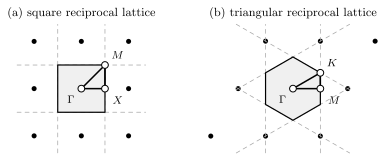
The first zone is bounded by perpendicular bisectors to the nearest reciprocal points. The displayed square path is $\Gamma\!-\!X\!-\!M\!-\!\Gamma$; the triangular path is $\Gamma\!-\!M\!-\!K\!-\!\Gamma$. These labels are explicitly tied to the depicted reciprocal bases and should not be transferred to another convention without checking coordinates.

Square lattice

For a direct square lattice of period $a$,

$$\mathbf b_1 = \frac{2\pi}{a}(1,0), \qquad \mathbf b_2 = \frac{2\pi}{a}(0,1).$$

The first zone is

$$-\frac{\pi}{a} \leq k_x,k_y \leq \frac{\pi}{a},$$

with a half-open boundary convention understood when unique counting is required.

One common coordinate declaration is

$$\begin{aligned} \Gamma&=(0,0),\\ X&=\frac12\mathbf b_1,\\ M&=\frac12(\mathbf b_1+\mathbf b_2). \end{aligned}$$

$\Gamma$ is the zone center, $X$ is an edge midpoint, and $M$ is a corner.

Triangular reciprocal lattice

Choose reciprocal vectors of equal length meeting at $60^\circ$. The first zone is a regular hexagon. For the orientation in the figure, representative special points are

$$\begin{aligned} \Gamma&=\mathbf0,\\ M&=\frac12\mathbf b_1,\\ K&=\frac13(\mathbf b_1+\mathbf b_2). \end{aligned}$$

$M$ is an edge midpoint and $K$ is a corner. Their point-group stars contain all symmetry-equivalent edge midpoints and corners. A honeycomb crystal uses this same hexagonal first zone because its Bravais lattice is triangular; the two-site motif changes the bands, not the reciprocal translation lattice.

Three-Dimensional Shapes

The Wigner–Seitz construction extends directly to three dimensions:

• a simple-cubic direct lattice has a cubic reciprocal lattice and cubic first zone;
• an fcc direct lattice has a bcc reciprocal lattice and a truncated-octahedral first zone;
• a bcc direct lattice has an fcc reciprocal lattice and a rhombic-dodecahedral first zone.

For simple cubic,

$$-\frac{\pi}{a} \leq k_x,k_y,k_z \leq \frac{\pi}{a}.$$

A commonly used path includes

$$\begin{aligned} \Gamma&=(0,0,0),\\ X&=\frac{\pi}{a}(1,0,0),\\ M&=\frac{\pi}{a}(1,1,0),\\ R&=\frac{\pi}{a}(1,1,1). \end{aligned}$$

Noncubic zones can change shape as axial ratios vary even within the same broad lattice family. Automated band-path conventions therefore standardize the conventional cell, primitive basis, and metric case before assigning labels.

Point-Group Symmetry in the Zone

Let $\mathcal P$ be the reciprocal point group. It maps the reciprocal lattice to itself:

$$p\Lambda^* = \Lambda^*, \qquad p\in\mathcal P.$$

It also maps the first zone to itself. The star of $\mathbf k$ is

$$\operatorname{star}(\mathbf k) = \left\{ p\mathbf k \bmod\Lambda^* \;\middle|\; p\in\mathcal P \right\}.$$

All points in a star are symmetry related when the full Hamiltonian has that point-group symmetry.

Little group

The little co-group of $\mathbf k$ consists of operations satisfying

$$p\mathbf k = \mathbf k+\mathbf G_p$$

for some reciprocal vector $\mathbf G_p$. Generic interior points usually have the smallest little group. Zone centers, face centers, edges, corners, and special lines can have larger little groups and therefore stronger constraints on energies and eigenstates.

High-symmetry does not mean “highest energy,” “lowest energy,” or “most important for every observable.” It means that the wavevector is fixed modulo a reciprocal vector by more symmetry operations than a nearby generic point.

Irreducible Brillouin zone

An irreducible Brillouin zone is a region containing one representative from each point-group star. For a symmetry-invariant scalar integrand,

$$\frac{1}{\Omega_{\mathrm{BZ}}} \int_{\mathcal B_1} d^dk\, f(\mathbf k) \approx \sum_{\nu} w_\nu f(\mathbf k_\nu), \qquad \sum_\nu w_\nu=1,$$

after a suitable symmetry-weighted discretization.

The weights account for star sizes and boundary stabilizers. One cannot simply multiply an arbitrary wedge integral by the point-group order when boundary points, magnetic symmetry, spinor operations, or a nonsymmetric mesh are involved.

Time-reversal symmetry can relate $\mathbf k$ and $-\mathbf k$. In magnetic or driven systems it may be absent, and antiunitary symmetry must be handled separately from the ordinary point group.

High-Symmetry Labels and Paths

$\Gamma$ universally denotes $\mathbf k=\mathbf0$. Other labels such as $X$, $M$, $K$, $L$, $W$, $H$, and $R$ are conventional, not self-defining. Their coordinates can depend on:

• Bravais type and space group;
• conventional-cell setting and primitive basis;
• reciprocal-vector order and orientation;
• axial-ratio regime;
• whether spin, magnetism, or nonsymmorphic symmetry is included;
• the selected path standard.

A reproducible band plot should therefore declare the structure, space group or layer group, direct and reciprocal bases, fractional coordinates of every labeled point, and the path convention.

Authoritative machine-readable standards include the Bilbao Crystallographic Server k-vector database, the AFLOW convention, and the crystallographic convention implemented by SeeK-path. Their labels and recommended paths are not interchangeable in every setting.

What a path coordinate means

For vertices $\mathbf k_0,\mathbf k_1,\ldots$, a plotting coordinate is often accumulated reciprocal-space distance:

$$s_j = \sum_{\ell<j} \left| \mathbf k_{\ell+1} - \mathbf k_\ell \right|.$$

Within a segment,

$$\mathbf k(t) = (1-t)\mathbf k_j + t\mathbf k_{j+1}, \qquad 0\leq t\leq1.$$

The horizontal axis in a band diagram is then path distance $s$, not a Cartesian component such as $k_x$. At a corner where the path direction changes, left and right slopes probe different directional derivatives.

Some plotting tools assign equal visual width to each segment instead of using physical reciprocal distance. The displayed slope then cannot be read directly as a group velocity without reconstructing the actual $\mathbf k$ spacing.

Why Band Plots Use Special Paths

Special paths compress a multidimensional function $E_n(\mathbf k)$ into a readable one-dimensional diagram. They are valuable because:

• little-group representations label states and constrain degeneracies;
• symmetry-enforced crossings often occur on special points or lines;
• common conventions permit qualitative comparison among calculations;
• zone-center and boundary behavior becomes visible;
• computational cost is far lower than a dense full-zone visualization.

But a path is a set of measure zero inside a two- or three-dimensional zone. It can miss:

• a conduction-band minimum or valence-band maximum at generic $\mathbf k$;
• an indirect gap;
• a nodal loop or Weyl point away from the chosen line;
• a small Fermi pocket;
• avoided crossings displaced by symmetry breaking;
• anisotropy away from the plotted directions.

A high-symmetry band plot is not sufficient for a density of states, carrier concentration, Fermi surface, transport tensor, optical integral, Berry-curvature integral, or topological invariant. Those require an appropriate full-zone mesh or an adaptive calculation.

Reduced, Extended, and Repeated Schemes

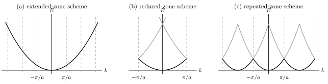
Three representations of one-dimensional reciprocal-space states. Panel (a) follows the free-electron parabola through successive zones. Panel (b) maps all wavevectors into the first zone and labels the folded branches as bands. Panel (c) repeats the reduced-zone bands in every reciprocal cell. The gray crossings remain ungapped because the illustrated particle is free.

Every wavevector $\mathbf q$ can be written

$$\mathbf q = \mathbf k+\mathbf G, \qquad \mathbf k\in\mathcal B_1.$$

The interior representative $\mathbf k$ is unique. Different plotting schemes decide whether to display $\mathbf q$, $\mathbf k$, or periodic copies of both.

Extended-zone scheme

The extended-zone scheme lets the displayed wavevector pass through successive Brillouin zones. It is useful for seeing how a nearly free branch evolves through Bragg planes and for connecting to scattering kinematics.

For a free particle, it is simply

$$E(\mathbf q) = \frac{\hbar^2|\mathbf q|^2}{2m}.$$

Each state is displayed once, but equivalent translation characters occur in different zones with different reciprocal offsets.

Reduced-zone scheme

The reduced-zone scheme maps every $\mathbf q$ into $\mathcal B_1$. The reciprocal offset becomes a branch or band label:

$$\varepsilon_{\mathbf G}^{(0)}(\mathbf k) = \frac{\hbar^2}{2m} |\mathbf k+\mathbf G|^2.$$

An infinite set of free parabolas is folded into the first zone. A periodic potential couples the folded branches and reorganizes them into bands. The reduced scheme is the natural representation for state counting, Brillouin-zone integration, and multiband Hamiltonians.

Repeated-zone scheme

The repeated-zone scheme copies the reduced-zone spectrum into every reciprocal cell:

$$\{E_n(\mathbf k+\mathbf G)\}_n = \{E_n(\mathbf k)\}_n.$$

The equality is safest as an equality of spectra. Depending on basis embedding, gauge, and degeneracies, individual band labels or Hamiltonian matrices can transform by a reciprocal sewing unitary rather than remain entry-by-entry identical.

Repeated-zone plots are useful for comparing several pockets, visualizing momentum-transfer processes, and overlaying experimental reciprocal-space maps.

These are representations, not approximations

Choosing reduced, extended, or repeated notation does not change the physical eigenstates. Confusing a plotting scheme with an approximation leads to false claims such as “zone folding creates a gap.” Folding changes labels; a perturbation that couples the folded sectors is needed to change eigenvalues.

Reciprocal Sewing and Basis Embedding

In the default cell convention, a Bloch Hamiltonian may be strictly periodic:

$$H(\mathbf k+\mathbf G) = H(\mathbf k).$$

In an orbital-embedded convention, define

$$\bigl[D_{\mathbf G}\bigr]_{\alpha\beta} = \delta_{\alpha\beta} e^{-i\mathbf G\cdot\boldsymbol\tau_\alpha}.$$

Then a common transformation law is

$$H(\mathbf k+\mathbf G) = D_{\mathbf G} H(\mathbf k) D_{\mathbf G}^{\dagger}.$$

The eigenvalues are periodic, while eigenvectors acquire basis-dependent phases. Berry connections and numerical overlaps are sensitive to this sewing convention even though gauge-invariant observables are not.

Conventions for Quantum Matter owns the cell-versus-orbital Fourier phases and reciprocal-boundary sewing rules.

State Counting and Zone Integrals

For a finite periodic crystal with $N_{\mathrm c}$ primitive cells, each isolated band contains $N_{\mathrm c}$ crystal-momentum states before spin or other internal multiplicities.

The thermodynamic replacement is

$$\frac{1}{N_{\mathrm c}} \sum_{\mathbf k\in\mathcal B_1} f(\mathbf k) \longrightarrow \frac{\Omega_{\mathrm c}}{(2\pi)^d} \int_{\mathcal B_1} d^dk\, f(\mathbf k).$$

Because

$$\frac{\Omega_{\mathrm c}}{(2\pi)^d} \operatorname{vol}(\mathcal B_1) = 1,$$

a constant integrand averages to itself. In a sample of physical measure $V=N_{\mathrm c}\Omega_{\mathrm c}$,

$$\sum_{\mathbf k} \longrightarrow \frac{V}{(2\pi)^d} \int_{\mathcal B_1} d^dk.$$

These normalizations are the bridge from band sums to particle density, total energy, response, and density of states.

Mesh choices

A uniform mesh can be written

$$\mathbf k_{\mathbf n} = \sum_{i=1}^{d} \frac{n_i+\eta_i}{N_i} \mathbf b_i,$$

where offsets $\eta_i$ specify centered or shifted sampling. A symmetry-reduced mesh assigns each irreducible point a weight equal to the number of represented full-zone points, adjusted at boundaries.

Convergence must be tested for the observable. Metals, small pockets, sharp Berry-curvature features, van Hove singularities, and near-degenerate bands can require much denser or adaptive meshes than a gapped total-energy calculation.

Zone Folding From Supercells and Order

Suppose a new direct cell contains

$$q=|\det S|$$

primitive cells:

$$A_{\mathrm s} = AS.$$

Its reciprocal basis is

$$B_{\mathrm s} = B S^{-\mathsf T},$$

and its Brillouin-zone volume is

$$\Omega_{\mathrm{BZ}}^{(\mathrm s)} = \frac{1}{q} \Omega_{\mathrm{BZ}}.$$

The smaller supercell zone receives $q$ folded branches for each primitive-cell band.

Two situations must be distinguished:

1. Computational supercell only. The physical Hamiltonian still has primitive translations. Folding is redundant bookkeeping, and primitive crystal momentum remains a hidden exact label.
2. Physical enlarged period. Structural, magnetic, charge, or orbital order genuinely reduces translation symmetry. States separated by new reciprocal vectors can hybridize, and new gaps or reconstructed pockets may appear.

Band unfolding estimates how much primitive-cell spectral character a supercell eigenstate carries. It is a projection with weights, not an exact restoration of a symmetry that the physical system has broken.

When the Ordinary Zone Needs Modification

The ordinary Brillouin zone assumes exact discrete translations.

Situation	Appropriate modification
commensurate superstructure	use the enlarged real cell and folded zone
antiferromagnetic or density-wave order	use the translation group of the ordered phase
uniform magnetic field with rational flux	use magnetic translations and a magnetic Brillouin zone
surface or interface	preserve only translations parallel to the surface and use a projected surface zone
finite open sample	crystal momentum is approximate away from boundaries
disorder	use spectral functions, configuration averages, or unfolded momentum weight
incommensurate structure	use approximants or higher-dimensional formulations with declared limits
quasicrystal	no ordinary finite reciprocal primitive cell exists

In an interacting many-body system, total crystal momentum still labels translation sectors when symmetry is exact, but a single-particle band $E_n(\mathbf k)$ need not describe the excitations. Zone geometry survives more generally than independent-electron band theory.

Common Mistakes

Mistake	Correction
calling any reciprocal primitive cell “the first Brillouin zone”	the first zone is specifically the Wigner–Seitz cell around the reciprocal origin
treating the zone boundary as a physical edge	boundary pieces are identified modulo reciprocal vectors
counting both equivalent faces on a finite mesh	adopt a half-open convention or merge reciprocal duplicates
assuming every boundary crossing opens a gap	hybridization must be allowed and have a nonzero coupling
reading $X$, $M$, or $K$ without coordinates	labels depend on lattice, setting, basis, and path standard
interpreting the band-plot horizontal axis as $k_x$	it is usually cumulative distance along a piecewise path
inferring a full gap from a high-symmetry path	generic off-path extrema can close it
computing a density of states from path samples	use a full-zone integration mesh
saying folding alone changes the spectrum	relabeling folds; a physical perturbation hybridizes
confusing the finite $\mathbf k$ mesh with reciprocal-lattice points	mesh points sample one zone; $\mathbf G$ identifies equivalent classes
assuming Hamiltonian matrices are strictly periodic in every basis	orbital embedding can produce unitary reciprocal sewing

Exercises

Exercise 1: half-space construction

Starting from

$$|\mathbf k| \leq |\mathbf k-\mathbf G|,$$

derive the Bragg-plane inequality and explain why $\mathbf G$ and $-\mathbf G$ bound opposite sides of the zone.

Solution

Squaring gives

$$|\mathbf k|^2 \leq |\mathbf k|^2 - 2\mathbf k\cdot\mathbf G + |\mathbf G|^2.$$

Therefore

$$\mathbf k\cdot\mathbf G \leq \frac{|\mathbf G|^2}{2}.$$

Replacing $\mathbf G$ by $-\mathbf G$ gives

$$-\mathbf k\cdot\mathbf G \leq \frac{|\mathbf G|^2}{2},$$

or

$$\mathbf k\cdot\mathbf G \geq -\frac{|\mathbf G|^2}{2}.$$

Together the pair confines the projection of $\mathbf k$ along $\mathbf G$ between two opposite perpendicular bisectors.

Exercise 2: square-zone coordinates

For a direct square lattice of period $a$, verify the coordinates of $\Gamma$, $X$, and $M$ above. Compute the path lengths $|\Gamma X|$, $|XM|$, and $|M\Gamma|$.

Solution

The reciprocal vectors are

$$\mathbf b_1 = \frac{2\pi}{a}(1,0), \qquad \mathbf b_2 = \frac{2\pi}{a}(0,1).$$

Thus

$$X=\frac{\pi}{a}(1,0), \qquad M=\frac{\pi}{a}(1,1).$$

The segment lengths are

$$|\Gamma X| = \frac{\pi}{a}, \qquad |XM| = \frac{\pi}{a}, \qquad |M\Gamma| = \frac{\sqrt2\pi}{a}.$$

A band plot using physical cumulative distance should therefore draw the diagonal segment longer than either edge segment.

Exercise 3: finite state count

A $d$-dimensional periodic crystal has $N_i$ cells along $\mathbf a_i$. Show that one Brillouin zone contains $N_{\mathrm c}=\prod_iN_i$ allowed crystal momenta and derive the continuum sum normalization.

Solution

The allowed points are

$$\mathbf k_{\mathbf m} = \sum_i \frac{m_i}{N_i}\mathbf b_i,$$

with $N_i$ inequivalent values of each $m_i$ modulo $N_i$. Their product is

$$N_{\mathrm c} = \prod_iN_i.$$

Each point occupies reciprocal measure

$$\Delta\Omega_k = \frac{\Omega_{\mathrm{BZ}}}{N_{\mathrm c}} = \frac{(2\pi)^d} {N_{\mathrm c}\Omega_{\mathrm c}}.$$

Hence

$$\sum_{\mathbf k}f(\mathbf k) \longrightarrow \frac{N_{\mathrm c}}{\Omega_{\mathrm{BZ}}} \int_{\mathcal B_1}d^dk\,f(\mathbf k) = \frac{V}{(2\pi)^d} \int_{\mathcal B_1}d^dk\,f(\mathbf k),$$

where $V=N_{\mathrm c}\Omega_{\mathrm c}$.

Exercise 4: boundary gap

At a free-electron Bragg plane, diagonalize

$$H = \begin{pmatrix} \varepsilon_0&V_{\mathbf G}\\ V_{\mathbf G}^*&\varepsilon_0 \end{pmatrix}.$$

What happens if symmetry forces $V_{\mathbf G}=0$?

Solution

The characteristic equation is

$$\bigl(E-\varepsilon_0\bigr)^2 - |V_{\mathbf G}|^2 = 0.$$

Therefore

$$E_\pm = \varepsilon_0 \pm |V_{\mathbf G}|,$$

and the splitting is

$$\Delta E = 2|V_{\mathbf G}|.$$

If $V_{\mathbf G}=0$, this two-state coupling does not lift the crossing. Other states or higher-order processes may still matter, but the geometric fact that the point lies on a zone boundary does not itself create a gap.

Exercise 5: doubling a one-dimensional cell

A one-dimensional Hamiltonian initially has period $a$. It is represented in a cell of length $2a$. Find the new zone and identify which primitive-zone wavevectors fold together.

Solution

The primitive reciprocal vector is

$$G = \frac{2\pi}{a}.$$

The doubled-cell reciprocal vector is

$$G_{\mathrm s} = \frac{2\pi}{2a} = \frac{\pi}{a}.$$

The new first zone is

$$-\frac{\pi}{2a} \leq k < \frac{\pi}{2a}.$$

Primitive-zone labels separated by $G_{\mathrm s}=\pi/a$ map to the same supercell label:

$$k \quad\text{and}\quad k+\frac{\pi}{a}.$$

If $2a$ is only a computational choice, the two folded sectors cannot hybridize under a Hamiltonian that still respects translation by $a$. If a real dimerization breaks the $a$ translation, coupling between them is allowed and a gap can open at the new boundary.

Exercise 6: path data are incomplete

Explain why agreement of two band models on a finite collection of high-symmetry line segments does not imply agreement throughout a two-dimensional Brillouin zone.

Solution

A finite collection of line segments has zero area inside the two-dimensional zone. One can construct a smooth periodic function $f(\mathbf k)$ that vanishes on every selected segment but is nonzero in a small region away from them. If

$$E_2(\mathbf k) = E_1(\mathbf k) + \lambda f(\mathbf k),$$

then the two dispersions agree exactly on the plotted path for every $\lambda$, yet differ elsewhere. The perturbation can create an off-path extremum, pocket, or crossing without changing the displayed path.

Symmetry can relate additional points, but it does not turn a one-dimensional path into a full two-dimensional sampling. Full-zone claims require full-zone evidence.

Exercise 7: sewing across a reciprocal boundary

Show that the orbital-embedded transformation

$$H(\mathbf k+\mathbf G) = D_{\mathbf G} H(\mathbf k) D_{\mathbf G}^{\dagger}$$

preserves eigenvalues. What information can still change?

Solution

$D_{\mathbf G}$ is diagonal and unitary because each entry has unit magnitude:

$$D_{\mathbf G}^{\dagger}D_{\mathbf G} = I.$$

Unitary conjugation preserves the characteristic polynomial:

$$\det \left[ E- D_{\mathbf G}H D_{\mathbf G}^{\dagger} \right] = \det \left[ D_{\mathbf G}(E-H)D_{\mathbf G}^{\dagger} \right] = \det(E-H).$$

Thus the eigenvalue set is unchanged. Eigenvector components, orbital phases, Berry connections, and raw overlap matrices can change. Gauge-covariant or gauge-invariant combinations must include the sewing unitary when crossing the zone boundary.

Connections

• The chapter gateway routes Brillouin-zone geometry onward to the appropriate theorem, band construction, or band-derived output.
• Reciprocal Lattice derives the reciprocal basis, metric, cell measure, diffraction condition, and $\mathbf k\sim\mathbf k+\mathbf G$ equivalence used here.
• Crystals and Lattices fixes the primitive direct translation cell that determines the zone volume.
• Crystalline Symmetry Preview introduces little groups, translation characters, and point-group constraints.
• Symmetry of Bloch States starts from the stars and little co-groups defined here and owns their representations, compatibility relations, and degeneracy or crossing constraints.
• Boundary Conditions on Lattices explains how finite periodic geometry produces a discrete zone mesh.
• Berry Phase and Chern Numbers use the global topology and boundary sewing of the Brillouin torus; Chern Numbers in Band Theory implements the occupied-projector integral and periodic mesh computation.
• Bloch’s Theorem is the next canonical step and constructs states carrying these translation characters.
• Nearly Free Electrons explains why weak periodic potentials matter most on the Bragg planes that bound the zones.
• Moiré Superlattices applies reduced-zone bookkeeping to long-wavelength registry patterns, mini Brillouin zones, and hybridized minibands.

References

• M. I. Aroyo et al., “Brillouin-zone database on the Bilbao Crystallographic Server,” Acta Crystallographica A 70, 126–137 (2014), doi:10.1107/S205327331303091X.
• N. W. Ashcroft and N. D. Mermin, Solid State Physics (Holt, Rinehart and Winston, 1976), Chapters 5–9.
• L. Brillouin, Wave Propagation in Periodic Structures, 2nd ed. (Dover, 1953).
• Y. Hinuma, G. Pizzi, Y. Kumagai, F. Oba, and I. Tanaka, “Band structure diagram paths based on crystallography,” Computational Materials Science 128, 140–184 (2017), doi:10.1016/j.commatsci.2016.10.015.
• H. Jones, The Theory of Brillouin Zones and Electronic States in Crystals (North-Holland, 1960).
• C. Kittel, Introduction to Solid State Physics, 8th ed. (Wiley, 2004), Chapters 2 and 7.
• M. P. Marder, Condensed Matter Physics, 2nd ed. (Wiley, 2010), Chapters 2–4.
• H. J. Monkhorst and J. D. Pack, “Special points for Brillouin-zone integrations,” Physical Review B 13, 5188–5192 (1976), doi:10.1103/PhysRevB.13.5188.
• W. Setyawan and S. Curtarolo, “High-throughput electronic band structure calculations: Challenges and tools,” Computational Materials Science 49, 299–312 (2010), doi:10.1016/j.commatsci.2010.05.010.
• S. H. Simon, The Oxford Solid State Basics (Oxford University Press, 2013), Chapters 5–7.
• M. Tinkham, Group Theory and Quantum Mechanics (Dover, 2003), Chapters 5–6.