Reciprocal Lattice

The reciprocal lattice is the set of wavevectors whose plane-wave phase is unchanged by every direct-lattice translation. If $\Lambda$ is the direct lattice, then the physics-normalized reciprocal lattice is

$$\Lambda^* = \left\{ \mathbf G\in\mathbb R^d \;\middle|\; e^{i\mathbf G\cdot\mathbf R}=1 \text{ for every }\mathbf R\in\Lambda \right\}.$$

This definition unifies three facts that can otherwise look unrelated:

• a lattice-periodic function has Fourier components only at reciprocal-lattice vectors;
• elastic diffraction from a perfect crystal is concentrated where the wavevector transfer equals a reciprocal vector;
• translation symmetry conserves crystal momentum only modulo a reciprocal vector.

Crystals and Lattices owns the direct-space translation group and motif. This page constructs its dual lattice. The first Brillouin zone, zone boundaries, and reduced-zone bookkeeping belong to the next article.

Required background. Crystals and Lattices supplies primitive translations, cells, motifs, and cell volume.

Helpful background. Fourier Series supplies the reciprocal-mode expansion of lattice-periodic functions.

Definition From Phase Invariance

Let the direct lattice be

$$\Lambda = \left\{ \mathbf R = \sum_{i=1}^{d}n_i\mathbf a_i \;\middle|\; n_i\in\mathbb Z \right\}.$$

A plane wave changes under $\mathbf r\mapsto\mathbf r+\mathbf R$ by

$$e^{i\mathbf q\cdot(\mathbf r+\mathbf R)} = e^{i\mathbf q\cdot\mathbf r} e^{i\mathbf q\cdot\mathbf R}.$$

It is lattice-periodic precisely when

$$e^{i\mathbf q\cdot\mathbf R}=1 \qquad \text{for all }\mathbf R\in\Lambda.$$

Since $e^{ix}=1$ exactly when $x\in2\pi\mathbb Z$, the reciprocal lattice can also be written

$$\Lambda^* = \left\{ \mathbf G \;\middle|\; \mathbf G\cdot\mathbf R \in 2\pi\mathbb Z \text{ for every }\mathbf R\in\Lambda \right\}.$$

It is enough to test the primitive translations:

$$\mathbf a_i\cdot\mathbf G \in 2\pi\mathbb Z \qquad i=1,\ldots,d.$$

If this condition holds for every $\mathbf a_i$, then it holds for every integer combination $\mathbf R$. Conversely, each $\mathbf a_i$ is itself a lattice vector, so the full definition implies the primitive conditions.

Group structure

If $\mathbf G,\mathbf G'\in\Lambda^*$, then

$$e^{i(\mathbf G+\mathbf G')\cdot\mathbf R} = e^{i\mathbf G\cdot\mathbf R} e^{i\mathbf G'\cdot\mathbf R} = 1.$$

The zero vector and additive inverses also satisfy the condition. Thus $\Lambda^*$ is itself an abelian lattice under vector addition.

The definition depends on the direct translation lattice, not directly on the atomic species or motif. A motif changes Fourier amplitudes at reciprocal points and can extinguish some peaks, but it does not change the reciprocal lattice of the primitive translations.

Why Fourier Analysis Produces a Lattice

Let $f(\mathbf r)$ be periodic under every $\mathbf R\in\Lambda$. Expand it in plane waves:

$$f(\mathbf r) = \int \frac{d^dq}{(2\pi)^d} \widetilde f(\mathbf q) e^{i\mathbf q\cdot\mathbf r}.$$

Periodicity requires

$$f(\mathbf r+\mathbf R) = f(\mathbf r).$$

Every nonzero Fourier component must therefore have

$$e^{i\mathbf q\cdot\mathbf R}=1 \qquad \text{for all }\mathbf R\in\Lambda.$$

The continuum Fourier integral reduces to a reciprocal-lattice series:

$$f(\mathbf r) = \sum_{\mathbf G\in\Lambda^*} f_{\mathbf G} e^{i\mathbf G\cdot\mathbf r}.$$

With a primitive cell $\mathcal C$ of measure $\Omega_{\mathrm c}$,

$$f_{\mathbf G} = \frac{1}{\Omega_{\mathrm c}} \int_{\mathcal C} d^dr\, e^{-i\mathbf G\cdot\mathbf r} f(\mathbf r).$$

The orthogonality relation is

$$\frac{1}{\Omega_{\mathrm c}} \int_{\mathcal C} d^dr\, e^{i(\mathbf G-\mathbf G')\cdot\mathbf r} = \delta_{\mathbf G,\mathbf G'}.$$

This is ordinary Fourier-series orthogonality on the quotient space $\mathbb R^d/\Lambda$. Periodic Functions and Fourier Series supplies the general analysis; the reciprocal lattice is its crystal-geometric realization.

Reciprocal Basis Vectors

Define reciprocal primitive vectors $\mathbf b_j$ by

$$\mathbf a_i\cdot\mathbf b_j = 2\pi\delta_{ij}.$$

Every reciprocal vector is then

$$\mathbf G = \sum_{j=1}^{d}m_j\mathbf b_j, \qquad m_j\in\mathbb Z.$$

Indeed,

$$\mathbf a_i\cdot\mathbf G = 2\pi m_i.$$

Conversely, any vector satisfying the phase-invariance definition has integer coefficients in this reciprocal basis.

Matrix construction

Put the direct and reciprocal vectors into column matrices:

$$\begin{aligned} A&= \begin{pmatrix} \mathbf a_1&\cdots&\mathbf a_d \end{pmatrix}, \\ B&= \begin{pmatrix} \mathbf b_1&\cdots&\mathbf b_d \end{pmatrix}. \end{aligned}$$

The defining relation becomes

$$A^{\mathsf T}B = 2\pi I_d.$$

Therefore

$$B = 2\pi A^{-\mathsf T}.$$

This is the most reliable formula for numerical work. It handles skew cells without guessing which reciprocal vector is perpendicular to which direct vector.

Three-dimensional cross products

For a right-handed direct basis,

$$\Omega_{\mathrm c} = \mathbf a_1\cdot \bigl(\mathbf a_2\times\mathbf a_3\bigr) > 0.$$

The reciprocal basis is

$$\begin{aligned} \mathbf b_1 &= 2\pi \frac{\mathbf a_2\times\mathbf a_3} {\Omega_{\mathrm c}}, \\ \mathbf b_2 &= 2\pi \frac{\mathbf a_3\times\mathbf a_1} {\Omega_{\mathrm c}}, \\ \mathbf b_3 &= 2\pi \frac{\mathbf a_1\times\mathbf a_2} {\Omega_{\mathrm c}}. \end{aligned}$$

Each $\mathbf b_i$ is perpendicular to the plane spanned by the other two direct vectors. It is not generally parallel to $\mathbf a_i$.

Two dimensions

For a right-handed two-dimensional basis embedded in the $xy$ plane,

$$\Omega_{\mathrm c} = \bigl( \mathbf a_1\times\mathbf a_2 \bigr)\cdot\hat{\mathbf z} > 0.$$

A convenient construction is

$$\begin{aligned} \mathbf b_1 &= \frac{2\pi}{\Omega_{\mathrm c}} \mathbf a_2\times\hat{\mathbf z}, \\ \mathbf b_2 &= \frac{2\pi}{\Omega_{\mathrm c}} \hat{\mathbf z}\times\mathbf a_1. \end{aligned}$$

Reversing the ordered orientation changes the corresponding signs. The invariant check is always $A^{\mathsf T}B=2\pi I$.

Direct and Reciprocal Geometry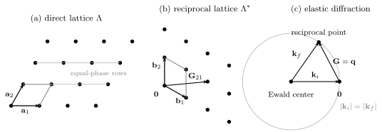

Direct and reciprocal lattices are dual under phase pairing. In panel (b), $\mathbf G_{21}=2\mathbf b_1+\mathbf b_2$. In panel (c), the reciprocal point lies on the elastic Ewald circle, so $\mathbf q=\mathbf k_f-\mathbf k_i=\mathbf G$ with $|\mathbf k_i|=|\mathbf k_f|$. The circle is two-dimensional shorthand for the Ewald sphere.

The reciprocal lattice reverses length scales. A large direct-space period produces closely spaced reciprocal points, while a short direct-space period produces a large reciprocal spacing.

Reciprocal-cell measure

Because $B=2\pi A^{-\mathsf T}$,

$$\Omega^* = \left|\det B\right| = \frac{(2\pi)^d}{\Omega_{\mathrm c}}.$$

Here $\Omega^*$ is the measure of any primitive reciprocal cell. The first Brillouin zone is one such cell, so the convention page denotes the same measure by $\Omega_{\mathrm{BZ}}$.

The units are inverse length to the power $d$. The product

$$\Omega_{\mathrm c}\Omega^* = (2\pi)^d$$

is basis independent.

Reciprocal metric

The direct metric is

$$g=A^{\mathsf T}A.$$

The reciprocal metric is

$$\begin{aligned} g^* &= B^{\mathsf T}B \\ &= (2\pi)^2g^{-1}. \end{aligned}$$

For integer index vector $\mathbf m$,

$$|\mathbf G_{\mathbf m}|^2 = \mathbf m^{\mathsf T} g^* \mathbf m.$$

This formula converts crystallographic indices into reciprocal-vector lengths for an arbitrary skew cell.

Change of primitive basis

If

$$A'=AM, \qquad M\in\operatorname{GL}(d,\mathbb Z),$$

then

$$B' = B M^{-\mathsf T}.$$

The new reciprocal vectors generate the same $\Lambda^*$ because $M^{-\mathsf T}$ is also an integer unimodular matrix. Individual basis vectors and integer coordinates change, but the reciprocal point set does not.

Reciprocal of the reciprocal

Applying the same $2\pi$-normalized construction to $B$ gives

$$2\pi B^{-\mathsf T} = A.$$

Thus

$$\bigl(\Lambda^*\bigr)^* = \Lambda$$

after identifying the double-dual Euclidean space with the original space.

Worked Examples

One-dimensional chain

For

$$\mathbf a_1=a\hat{\mathbf x},$$

the reciprocal primitive vector is

$$\mathbf b_1 = \frac{2\pi}{a}\hat{\mathbf x}.$$

Hence

$$G_m = \frac{2\pi m}{a}, \qquad m\in\mathbb Z.$$

The reciprocal spacing $2\pi/a$ is the angular spatial frequency of a pattern with period $a$.

Rectangular and square lattices

For

$$\mathbf a_1=a\hat{\mathbf x}, \qquad \mathbf a_2=c\hat{\mathbf y},$$

one finds

$$\mathbf b_1 = \frac{2\pi}{a}\hat{\mathbf x}, \qquad \mathbf b_2 = \frac{2\pi}{c}\hat{\mathbf y}.$$

The reciprocal of a rectangular lattice is rectangular. If $a=c$, both direct and reciprocal lattices are square, with reciprocal lattice constant $2\pi/a$.

Triangular lattice

Take

$$\begin{aligned} \mathbf a_1&=a(1,0),\\ \mathbf a_2&=a \left( \frac12,\frac{\sqrt3}{2} \right). \end{aligned}$$

Solving the duality equations gives

$$\begin{aligned} \mathbf b_1 &= \frac{2\pi}{a} \left( 1,-\frac{1}{\sqrt3} \right), \\ \mathbf b_2 &= \frac{2\pi}{a} \left( 0,\frac{2}{\sqrt3} \right). \end{aligned}$$

Both have length

$$|\mathbf b_1| = |\mathbf b_2| = \frac{4\pi}{\sqrt3a},$$

and their mutual angle is $120^\circ$. The reciprocal lattice is again triangular, rotated relative to the displayed direct basis.

Simple cubic lattice

For $\mathbf a_i=a\hat{\mathbf e}_i$,

$$\mathbf b_i = \frac{2\pi}{a}\hat{\mathbf e}_i.$$

The reciprocal lattice is simple cubic. A reciprocal vector indexed by $(h,k,l)$ is

$$\mathbf G_{hkl} = \frac{2\pi}{a} \bigl( h\hat{\mathbf x} + k\hat{\mathbf y} + l\hat{\mathbf z} \bigr).$$

Face-centered and body-centered duality

Use primitive vectors for a face-centered cubic direct lattice with conventional cubic parameter $a$:

$$\begin{aligned} \mathbf a_1&=\frac a2(0,1,1),\\ \mathbf a_2&=\frac a2(1,0,1),\\ \mathbf a_3&=\frac a2(1,1,0). \end{aligned}$$

The reciprocal primitive vectors are

$$\begin{aligned} \mathbf b_1&=\frac{2\pi}{a}(-1,1,1),\\ \mathbf b_2&=\frac{2\pi}{a}(1,-1,1),\\ \mathbf b_3&=\frac{2\pi}{a}(1,1,-1). \end{aligned}$$

These generate a body-centered cubic reciprocal lattice with conventional reciprocal parameter $4\pi/a$. Conversely, the reciprocal of a body-centered cubic direct lattice is face-centered cubic.

The statement concerns primitive translation lattices. If one starts from a nonprimitive conventional cubic cell, extra Fourier-grid points appear and centering factors extinguish the ones that are not in the true reciprocal lattice.

Lattice Planes and Miller Indices

For integer indices $(h,k,l)$, define

$$\mathbf G_{hkl} = h\mathbf b_1 + k\mathbf b_2 + l\mathbf b_3.$$

The surfaces

$$\mathbf G_{hkl}\cdot\mathbf r = 2\pi n, \qquad n\in\mathbb Z,$$

are parallel planes normal to $\mathbf G_{hkl}$. Every direct-lattice point lies on one of these planes because

$$\mathbf G_{hkl}\cdot\mathbf R = 2\pi \bigl( hn_1+kn_2+ln_3 \bigr).$$

For coprime $h,k,l$, adjacent planes have separation

$$d_{hkl} = \frac{2\pi}{|\mathbf G_{hkl}|}.$$

To see this, move by $\Delta\mathbf r=d\,\widehat{\mathbf G}$ between adjacent planes:

$$\mathbf G\cdot\Delta\mathbf r = |\mathbf G|d = 2\pi.$$

For a simple-cubic lattice,

$$d_{hkl} = \frac{a} {\sqrt{h^2+k^2+l^2}}.$$

Miller indices depend on the chosen crystallographic basis, while the physical plane normal and spacing do not. A bar over an index denotes a negative integer, such as $(1\bar10)$.

The 2π Convention

Two reciprocal-space conventions are standard.

Context	Duality relation	Plane-wave phase
condensed-matter physics	$\mathbf a_i\cdot\mathbf b_j=2\pi\delta_{ij}$	$e^{i\mathbf G\cdot\mathbf r}$
much of crystallography	$\mathbf a_i\cdot\mathbf a_j^*=\delta_{ij}$	$e^{2\pi i\mathbf g\cdot\mathbf r}$

They are related by

$$\mathbf b_i = 2\pi\mathbf a_i^*, \qquad \mathbf G = 2\pi\mathbf g.$$

In fractional coordinates $\mathbf r=A\boldsymbol\xi$,

$$e^{i\mathbf G_{hkl}\cdot\mathbf r} = e^{2\pi i \left( h\xi_1+k\xi_2+l\xi_3 \right)}.$$

This page and the rest of the volume use the physics convention. A quoted reciprocal coordinate in inverse ångströms is ambiguous until one knows whether it means cycles per length or radians per length. Conventions for Quantum Matter is the domain-wide notation contract.

Diffraction Condition

Suppose a probe scatters from an ideal crystal. Let $\mathbf k_i$ and $\mathbf k_f$ be incident and outgoing wavevectors, and define

$$\mathbf q = \mathbf k_f-\mathbf k_i.$$

With this sign convention, $\hbar\mathbf q$ is the probe’s momentum change; momentum conservation assigns $-\hbar\mathbf q$ to the sample when no other reservoir carries momentum. Some diffraction texts instead define the sample transfer as $\mathbf Q=\mathbf k_i-\mathbf k_f=-\mathbf q$. The sign choice does not change the reciprocal-lattice selection rule because $\Lambda^*$ is closed under $\mathbf G\mapsto-\mathbf G$. A scattering amplitude from equivalent cells contains the lattice sum

$$S_\Lambda(\mathbf q) = \sum_{\mathbf R\in\Lambda} e^{-i\mathbf q\cdot\mathbf R}.$$

For an infinite lattice, Poisson summation gives

$$\sum_{\mathbf R\in\Lambda} e^{-i\mathbf q\cdot\mathbf R} = \frac{(2\pi)^d}{\Omega_{\mathrm c}} \sum_{\mathbf G\in\Lambda^*} \delta^{(d)} \bigl( \mathbf q-\mathbf G \bigr).$$

Thus the coherent lattice contribution is concentrated at

$$\mathbf q=\mathbf G.$$

Because $\Lambda^*$ is closed under sign reversal, a source using $\mathbf q=\mathbf k_i-\mathbf k_f$ obtains the equivalent condition $\mathbf q=\mathbf G$ with relabeled $\mathbf G$.

For a finite crystal, the delta functions become peaks with widths inversely related to the sample dimensions. Disorder, strain, domains, thermal displacement, instrumental resolution, and finite correlation length further alter their shapes.

Ewald construction

For elastic scattering,

$$|\mathbf k_i| = |\mathbf k_f| = k.$$

Place the reciprocal-lattice origin at the tip of $\mathbf k_i$ when the tail of $\mathbf k_i$ is at the Ewald-sphere center. A reciprocal point produces an elastic reflection when it lies on the sphere of radius $k$. The vector from the reciprocal origin to that point is

$$\mathbf G = \mathbf k_f-\mathbf k_i.$$

The construction encodes both energy conservation and the reciprocal-lattice selection rule.

Bragg’s law

Let $\theta$ be the angle between the incident beam and a family of planes with spacing $d$. The scattering angle is $2\theta$, so elastic geometry gives

$$|\mathbf q| = 2k\sin\theta.$$

For the $n$th reciprocal harmonic normal to those planes,

$$|\mathbf G_n| = n\frac{2\pi}{d}.$$

Using $k=2\pi/\lambda$ and $\mathbf q=\mathbf G_n$ yields

$$2d\sin\theta = n\lambda.$$

The Laue condition $\mathbf q=\mathbf G$ and Bragg’s law are not competing theories. They are the same elastic interference condition written in vector and plane-spacing language.

Lattice Peaks Versus Motif Intensities

Let the ideal density be assembled from motif functions:

$$\rho(\mathbf r) = \sum_{\mathbf R,\alpha} f_\alpha \bigl( \mathbf r-\mathbf R-\boldsymbol\tau_\alpha \bigr).$$

Its Fourier transform factorizes:

$$\widetilde\rho(\mathbf q) = \underbrace{ \sum_{\mathbf R} e^{-i\mathbf q\cdot\mathbf R} }_{\text{lattice factor}} \underbrace{ \sum_\alpha f_\alpha(\mathbf q) e^{-i\mathbf q\cdot\boldsymbol\tau_\alpha} }_{F(\mathbf q)}.$$

The first factor produces reciprocal-lattice peak positions. The motif structure factor $F(\mathbf G)$ controls amplitudes and systematic extinctions. The measured intensity is proportional to $|F(\mathbf G)|^2$ only after the probe coupling, polarization, kinematics, multiplicity, absorption, motion, and instrument response are handled.

Centering extinction example

Represent a body-centered cubic lattice using a conventional simple-cubic cell with motif positions

$$\boldsymbol\tau_1=\mathbf0, \qquad \boldsymbol\tau_2 = \frac a2(1,1,1).$$

For identical scatterers,

$$\begin{aligned} F_{hkl} &\propto 1+ e^{-i\pi(h+k+l)} \\ &= 1+(-1)^{h+k+l}. \end{aligned}$$

The conventional-grid reflection vanishes when $h+k+l$ is odd. The surviving points, with even index sum, form the face-centered reciprocal lattice expected from the primitive bcc translation group.

This is why peak absence can reflect centering or motif interference rather than the absence of a reciprocal coordinate in a chosen nonprimitive grid. Structure Factors owns the general scattering observable.

Momentum Conservation Modulo a Reciprocal Vector

Consider a periodic potential

$$V(\mathbf r) = \sum_{\mathbf G} V_{\mathbf G} e^{i\mathbf G\cdot\mathbf r}.$$

Between continuum plane waves,

$$\langle\mathbf k'|V|\mathbf k\rangle \propto \sum_{\mathbf G} V_{\mathbf G} \delta^{(d)} \bigl( \mathbf k'-\mathbf k-\mathbf G \bigr).$$

The periodic potential couples wavevectors satisfying

$$\mathbf k' = \mathbf k+\mathbf G.$$

This is the simplest appearance of momentum conservation modulo the reciprocal lattice. A lattice translation cannot distinguish $\mathbf k$ from $\mathbf k+\mathbf G$ because

$$e^{i(\mathbf k+\mathbf G)\cdot\mathbf R} = e^{i\mathbf k\cdot\mathbf R}.$$

Bloch theory turns these equivalence classes into crystal-momentum labels.

Many-particle selection rule

A translation-invariant lattice interaction can scatter modes subject to

$$\mathbf k_1+\mathbf k_2 = \mathbf k_3+\mathbf k_4+\mathbf G.$$

The $\mathbf G=\mathbf0$ representation is often called a normal process. A process represented with nonzero $\mathbf G$ is called Umklapp after all external labels have been placed in a chosen Brillouin zone.

That classification depends on the zone representatives, but its transport consequences are real. Umklapp allows the crystal-momentum carried by a selected low-energy sector to change by a reciprocal vector, so a current need not be protected as if continuous mechanical momentum were conserved within that sector.

Wavevector is not mechanical momentum

$\hbar\mathbf k$ is the generator label associated with discrete translations. It is not generally the expectation value of the mechanical momentum operator. In a full isolated system, actual momentum accounting includes ions, fields, boundaries, and the apparatus. “The lattice absorbs $\hbar\mathbf G$” is useful shorthand only within a stated effective description.

Reciprocal Lattice Versus Finite Momentum Mesh

The reciprocal lattice and the allowed $\mathbf k$ points of a finite periodic sample are different sets.

For $N_i$ cells along $\mathbf a_i$, Born–von Karman boundary conditions require

$$e^{i\mathbf k\cdot N_i\mathbf a_i} = 1.$$

Allowed wavevectors can be chosen as

$$\mathbf k_{\mathbf m} = \sum_{i=1}^{d} \frac{m_i}{N_i} \mathbf b_i, \qquad m_i=0,\ldots,N_i-1.$$

There are

$$N_{\mathrm c} = \prod_iN_i$$

inequivalent points modulo $\Lambda^*$. Their spacing shrinks as the sample grows. By contrast, the reciprocal vectors $\mathbf G=\sum_i\ell_i\mathbf b_i$ are fixed by the primitive direct lattice and identify equivalent translation characters.

The finite orthogonality relation is

$$\frac{1}{N_{\mathrm c}} \sum_{\mathbf R} e^{i(\mathbf k-\mathbf k')\cdot\mathbf R} = \delta_{\mathbf k,\mathbf k'\bmod\Lambda^*}.$$

For a supercell matrix $S$ with

$$A_{\mathrm s}=AS,$$

the supercell reciprocal basis is

$$B_{\mathrm s} = B S^{-\mathsf T}.$$

The larger real-space supercell produces a finer reciprocal grid. The finite $\mathbf k$ mesh can be viewed as representatives of the quotient between the supercell reciprocal lattice and the primitive reciprocal lattice.

Numerical Construction and Checks

Given a direct-lattice matrix $A$:

1. verify its units, rank, column order, and orientation;
2. compute $B=2\pi A^{-\mathsf T}$;
3. check $A^{\mathsf T}B$ against $2\pi I$;
4. verify $|\det A|\,|\det B|=(2\pi)^d$;
5. generate $\mathbf G=B\mathbf m$ from bounded integer tuples;
6. sort vectors by $|\mathbf G|^2$ using the reciprocal metric;
7. transform indices with $M^{\mathsf T}$ when changing the direct primitive basis;
8. keep crystallographic no-$2\pi$ coordinates distinct from physics wavevectors.

For floating-point data, do not identify reciprocal vectors by exact Cartesian equality. Compare integer coordinates when possible, or use tolerances scaled to the reciprocal basis condition number.

An apparently singular or wildly large reciprocal basis often signals nearly linearly dependent direct vectors, inconsistent units, or a conventional-to-primitive conversion error.

Common Mistakes

Mistake	Correction
defining the reciprocal lattice as “momentum space”	it is a discrete dual lattice inside wavevector space
forgetting the $2\pi$ convention	state whether $\mathbf a_i\cdot\mathbf b_j$ is $2\pi\delta_{ij}$ or $\delta_{ij}$
assuming $\mathbf b_i\parallel\mathbf a_i$	this is generally false for nonorthogonal cells
constructing reciprocal vectors from a nonprimitive cell without centering conditions	use primitive translations or include the corresponding extinction rules
calling every finite allowed $\mathbf k$ a reciprocal vector	the finite mesh is finer; reciprocal vectors identify equivalent $\mathbf k$ labels
treating reciprocal points as guaranteed diffraction peaks	a motif structure factor can make the amplitude vanish
confusing $\mathbf q$ with physical momentum	for $\mathbf q=\mathbf k_f-\mathbf k_i$, $\hbar\mathbf q$ is the probe momentum change and $-\hbar\mathbf q$ is the sample transfer when no other reservoir participates
saying Bragg and Laue conditions are different mechanisms	they are scalar-plane and vector forms of the same elastic interference condition
conserving crystal momentum as an ordinary vector	lattice processes conserve it modulo $\mathbf G$
using a Brillouin zone as the definition of $\Lambda^*$	the reciprocal lattice comes first; a zone is a primitive cell of reciprocal space

Exercises

Exercise 1: equivalence of the definitions

Prove that

$$e^{i\mathbf G\cdot\mathbf R}=1 \quad \text{for every }\mathbf R\in\Lambda$$

if and only if

$$\mathbf G = \sum_i m_i\mathbf b_i, \qquad m_i\in\mathbb Z.$$

Solution

If $\mathbf G=\sum_jm_j\mathbf b_j$, then for $\mathbf R=\sum_in_i\mathbf a_i$,

$$\mathbf G\cdot\mathbf R = \sum_{i,j} m_jn_i \mathbf b_j\cdot\mathbf a_i = 2\pi\sum_i m_in_i.$$

The exponential is therefore one.

Conversely, expand an arbitrary $\mathbf G$ in the reciprocal vector-space basis:

$$\mathbf G = \sum_jc_j\mathbf b_j.$$

Phase invariance for $\mathbf R=\mathbf a_i$ gives

$$e^{2\pi i c_i}=1,$$

so every $c_i$ is an integer. Hence $\mathbf G\in\Lambda^*$.

Exercise 2: triangular reciprocal lattice

Derive the reciprocal basis for

$$\mathbf a_1=a(1,0), \qquad \mathbf a_2=a \left( \frac12,\frac{\sqrt3}{2} \right),$$

and verify its cell area.

Solution

The direct matrix and its inverse transpose give

$$A = a \begin{pmatrix} 1&1/2\\ 0&\sqrt3/2 \end{pmatrix},$$

and

$$B = 2\pi A^{-\mathsf T} = \frac{2\pi}{a} \begin{pmatrix} 1&0\\ -1/\sqrt3&2/\sqrt3 \end{pmatrix}.$$

The columns are the $\mathbf b_1,\mathbf b_2$ stated above. Since

$$\Omega_{\mathrm c} = \frac{\sqrt3}{2}a^2,$$

the reciprocal area should be

$$\Omega^* = \frac{(2\pi)^2}{\Omega_{\mathrm c}} = \frac{8\pi^2}{\sqrt3a^2}.$$

Taking the determinant of $B$ gives the same result.

Exercise 3: basis covariance

Let $A'=AM$ with $M\in\operatorname{GL}(d,\mathbb Z)$. Derive the reciprocal transformation and the transformation of integer reciprocal coordinates.

Solution

The new reciprocal matrix is

$$\begin{aligned} B' &= 2\pi(A')^{-\mathsf T} \\ &= 2\pi(AM)^{-\mathsf T} \\ &= B M^{-\mathsf T}. \end{aligned}$$

For the same geometric reciprocal vector,

$$\mathbf G = B\mathbf m = B'\mathbf m' = B M^{-\mathsf T}\mathbf m'.$$

Therefore

$$\mathbf m' = M^{\mathsf T}\mathbf m.$$

Because $M$ is unimodular, $\mathbf m'$ remains integral. The Cartesian vector and reciprocal lattice are unchanged even though their indexed coordinates differ.

Exercise 4: cubic plane spacing

For a simple-cubic lattice, show that the $(hkl)$ plane spacing is

$$d_{hkl} = \frac{a}{\sqrt{h^2+k^2+l^2}}.$$

Find $d_{100}$, $d_{110}$, and $d_{111}$.

Solution

The reciprocal vector is

$$\mathbf G_{hkl} = \frac{2\pi}{a}(h,k,l),$$

so

$$|\mathbf G_{hkl}| = \frac{2\pi}{a} \sqrt{h^2+k^2+l^2}.$$

Using $d_{hkl}=2\pi/|\mathbf G_{hkl}|$ gives the result. In particular,

$$d_{100}=a, \qquad d_{110}=\frac{a}{\sqrt2}, \qquad d_{111}=\frac{a}{\sqrt3}.$$

Exercise 5: derive Bragg’s law

An elastic probe has wavelength $\lambda$ and scatters through angle $2\theta$. Starting from $\mathbf q=\mathbf G_n$, derive Bragg’s law for planes of spacing $d$.

Solution

Elasticity gives $|\mathbf k_i|=|\mathbf k_f|=2\pi/\lambda$. The difference between equal-length vectors separated by angle $2\theta$ has magnitude

$$|\mathbf q| = 2|\mathbf k_i|\sin\theta = \frac{4\pi}{\lambda}\sin\theta.$$

The $n$th reciprocal harmonic normal to planes of spacing $d$ has

$$|\mathbf G_n| = \frac{2\pi n}{d}.$$

Equating magnitudes gives

$$\frac{4\pi}{\lambda}\sin\theta = \frac{2\pi n}{d},$$

or

$$2d\sin\theta=n\lambda.$$

Exercise 6: finite-lattice orthogonality

For a one-dimensional ring with $N$ cells, $R_n=na$ and $k_m=2\pi m/(Na)$. Show

$$\frac1N \sum_{n=0}^{N-1} e^{i(k_m-k_{m'})R_n} = \delta_{m,m'\bmod N}.$$

Solution

The sum is

$$\frac1N \sum_{n=0}^{N-1} \exp \left[ \frac{2\pi i}{N} (m-m')n \right].$$

If $m-m'$ is divisible by $N$, every term is one and the result is one. Otherwise it is a geometric series with ratio

$$z = e^{2\pi i(m-m')/N} \neq1$$

but $z^N=1$. Hence

$$\sum_{n=0}^{N-1}z^n = \frac{1-z^N}{1-z} = 0.$$

This finite Fourier orthogonality explains both the $N$ distinct momentum labels and their equivalence modulo $2\pi/a$.

Exercise 7: body-centered extinction

For identical scatterers at fractional conventional-cell positions $(0,0,0)$ and $(1/2,1/2,1/2)$, derive the reflection condition and explain its relation to the true reciprocal lattice.

Solution

In the crystallographic phase convention,

$$\begin{aligned} F_{hkl} &= f \left[ 1+ e^{-2\pi i \left( h/2+k/2+l/2 \right)} \right] \\ &= f \left[ 1+(-1)^{h+k+l} \right]. \end{aligned}$$

If $h+k+l$ is odd, the two amplitudes cancel. If it is even, they add to $2f$. Thus only conventional reciprocal-grid points with even index sum survive.

The conventional cubic vectors are not a primitive basis of the body-centered direct lattice. The surviving even-sum reciprocal points form a face-centered cubic lattice, which is precisely the reciprocal lattice obtained from a primitive bcc basis. The “extinctions” remove the extra grid points introduced by the nonprimitive cell.

Connections

• The chapter gateway distinguishes diffraction, Bloch, band-model, state-counting, and Fermi-surface routes before this dual-lattice derivation is used.
• Crystals and Lattices defines the direct translation group, primitive basis, motif, and finite-cell geometry used here.
• Poisson Summation Formula gives the distributional identity behind reciprocal delta peaks.
• Crystalline Symmetry Preview connects reciprocal equivalence to translation characters and point-group operations.
• Structure Factors develops the measured correlation function and separates coherent peaks from broader spectral weight.
• Electron Diffraction and X-Ray Experiments show how reciprocal-space conditions become evidence.
• X-Ray Scattering develops modern elastic, resonant, coherent, and inelastic photon-scattering practice.
• Brillouin Zones constructs the Wigner–Seitz reciprocal cell used to select one representative from each $\mathbf k\sim\mathbf k+\mathbf G$ class.

References

• J. Als-Nielsen and D. McMorrow, Elements of Modern X-Ray Physics, 2nd ed. (Wiley, 2011), Chapters 1–3.
• N. W. Ashcroft and N. D. Mermin, Solid State Physics (Holt, Rinehart and Winston, 1976), Chapters 5–7.
• A. Authier, Dynamical Theory of X-Ray Diffraction, rev. ed. (Oxford University Press, 2001), Chapters 1–3.
• J. M. Cowley, Diffraction Physics, 3rd ed. (North-Holland, 1995), Chapters 1–4.
• International Union of Crystallography, International Tables for Crystallography, especially Volumes A and C.
• C. Kittel, Introduction to Solid State Physics, 8th ed. (Wiley, 2004), Chapters 1–2.
• M. P. Marder, Condensed Matter Physics, 2nd ed. (Wiley, 2010), Chapters 1–3.
• S. H. Simon, The Oxford Solid State Basics (Oxford University Press, 2013), Chapters 4–6.
• B. Souvignier, “A general introduction to space groups,” International Tables for Crystallography A, Section 1.3.2.5 (2016), doi:10.1107/97809553602060000921. The International Tables use the no-$2\pi$ crystallographic reciprocal basis.
• G. L. Squires, Introduction to the Theory of Thermal Neutron Scattering, 3rd ed. (Cambridge University Press, 2012), Chapters 1–3.
• B. E. Warren, X-Ray Diffraction (Dover, 1990), Chapters 2–4.