X-Ray Scattering

X-ray scattering illuminates a sample with photons whose wavelength is comparable to an interatomic spacing, then records where the scattered photons go, how much energy they lose, and sometimes how their polarization changes. Far from an absorption edge, the leading elastic signal maps electron-density-weighted crystal structure. Near an edge, virtual core excitation makes the amplitude element, valence, orbital, and polarization selective. Coherent beams add speckle and phase-retrieval information, while energy analysis exposes phonons and electronic collective excitations.

Those capabilities do not make a detector image a direct picture of atoms or charge order. The measured counts combine the sample amplitude with flux, polarization, geometry, absorption, fluorescence, detector response, reciprocal-space acceptance, and resolution. In coherent diffraction, the detector ordinarily loses the scattered phase. Near resonance, the same edge that enhances contrast also changes attenuation and can make the scattering amplitude tensorial.

A useful evidence ladder is:

1. detector record: photon counts versus pixel, angle, sample orientation, incident energy, outgoing energy, polarization channel, and exposure;
2. calibrated coordinates: counts mapped to $\mathbf Q$, energy transfer, reciprocal-lattice units, and a documented detector mask;
3. corrected intensity: incident-flux normalization, dark and flat-field treatment, geometry, polarization, absorption, dead-time, and background corrections;
4. scattering inference: structure-factor amplitude, peak position and width, resonant tensor contrast, diffuse intensity, speckle correlation, or energy-loss spectrum under a resolution-convolved model;
5. material claim: crystal structure, displacement field, charge or orbital order, domain dynamics, phonon, magnon, or other collective excitation supported by symmetry tests and complementary probes.

An extra peak establishes scattering weight at a wavevector. It does not, by itself, identify which microscopic degree of freedom produced that weight.

Canonical Scope

This page is the canonical home for X-ray-scattering practice in quantum matter. It owns photon-transfer kinematics, elastic diffraction intensities, atomic and resonant form factors, laboratory and synchrotron workflows, absorption and fluorescence systematics, charge-order measurements, coherent diffraction and phase retrieval, and the experimental boundary between nonresonant inelastic X-ray scattering and resonant inelastic X-ray scattering.

Reciprocal Lattice owns reciprocal-basis construction, Miller indices, the Ewald construction, and the equivalence of Laue and Bragg conditions. Structure Factors owns static and dynamic correlation functions, normalization conventions, detailed balance, and sum rules. Charge and Spin Density Waves owns density-wave symmetry, mechanisms, reconstruction, and phase-level evidence. Phonons and Spin Waves and Magnons own the target excitations. This page explains how X-ray counts constrain those objects without duplicating their full theory.

The historical role of crystal diffraction, characteristic radiation, Moseley’s law, and Compton scattering belongs to X-Ray Experiments. Here the emphasis is modern condensed-matter measurement.

Photon Kinematics and Coupling

Wavelength, momentum, and energy transfer

For a photon in vacuum,

$$\lvert\mathbf k\rvert = \frac{2\pi}{\lambda} = \frac{E}{\hbar c}.$$

A convenient conversion is

$$\lambda[\mathrm{nm}] \simeq \frac{1.23984}{E[\mathrm{keV}]}.$$

Thus a $10\ \mathrm{keV}$ hard X-ray has $\lambda\simeq0.124\ \mathrm{nm}$, comparable with crystal spacings. Soft X-rays near transition-metal $L$ edges have longer wavelengths and lower penetration depths, but offer direct dipole access to valence-sensitive intermediate states.

Adopt the target-transfer convention

$$\mathbf Q = \mathbf k_i-\mathbf k_f, \qquad \hbar\omega = E_i-E_f.$$

Positive $\omega$ means that the sample gains energy. If $2\theta$ is the angle between incident and outgoing beams, elastic scattering has

$$Q = \frac{4\pi}{\lambda} \sin\theta.$$

The accessible reciprocal-space region is therefore set by photon energy, scattering angle, sample orientation, and mechanical shadowing. A nominally accessible reflection can still be blocked by a cryostat, pressure cell, beamstop, detector gap, or polarization geometry.

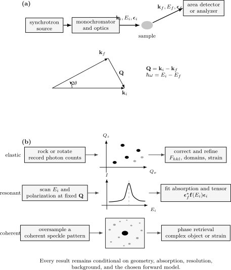
The same incident and outgoing photon variables support experimentally distinct reductions. Elastic diffraction maps reciprocal-space intensity and refines $F_{hkl}$; resonant scattering scans energy and polarization through a tensor amplitude; coherent diffraction oversamples speckles and reconstructs a constrained complex object. None of the three bypasses geometry, absorption, resolution, or background modeling.

Thomson amplitude and polarization

Far from an absorption edge and within the weak, single-scattering limit, one free electron contributes the Thomson cross section

$$\frac{d\sigma_{\mathrm T}}{d\Omega} = r_e^2 \left| \boldsymbol\epsilon_f^* \cdot \boldsymbol\epsilon_i \right|^2,$$

where

$$r_e = \frac{e^2}{4\pi\epsilon_0m_ec^2}$$

is the classical electron radius. The polarization factor is part of the forward model, not a cosmetic correction. Synchrotron radiation is usually strongly polarized, and an analyzer can separate outgoing polarization channels. Even without an analyzer, the detector sums only over the outgoing states admitted by its geometry.

For an isolated atom with electron number density $\rho_e(\mathbf r)$, the nonresonant amplitude in electron units is

$$f_0(\mathbf Q) = \int d^3r\, \rho_e(\mathbf r) e^{i\mathbf Q\cdot\mathbf r}, \qquad f_0(\mathbf 0)=Z.$$

Because the electron cloud has finite extent, $f_0(Q)$ generally decreases with $Q$. X-ray diffraction therefore weights heavy atoms strongly at small momentum transfer and can have weak contrast for light atoms beside heavy ones. This contrasts with neutron scattering lengths, which vary irregularly across elements and isotopes.

The expression above is a spherical, independent-atom baseline. Bonding charge, asphericity, magnetization, relativistic terms, and resonant transitions require more detailed amplitudes.

Crystal Structure from Elastic Diffraction

Lattice sum and unit-cell amplitude

Let $\mathbf R_n$ label unit cells and $\mathbf r_j$ the position of atom $j$ inside a cell. In the kinematic approximation, the elastic amplitude separates into

$$\mathcal A(\mathbf Q,E) = \sum_n e^{i\mathbf Q\cdot\mathbf R_n} F_{\mathrm{cell}}(\mathbf Q,E),$$

with

$$\begin{aligned} F_{\mathrm{cell}}(\mathbf Q,E) ={}& \sum_j o_j\, f_j(\mathbf Q,E)\, e^{-W_j(\mathbf Q)} \\ &\times e^{i\mathbf Q\cdot\mathbf r_j}. \end{aligned}$$

Here $o_j$ is occupancy, $f_j$ is the atomic or tensor scattering amplitude, and $e^{-W_j}$ is the amplitude Debye–Waller factor. For a Gaussian displacement tensor $U_j$,

$$W_j(\mathbf Q) = \frac{1}{2} \mathbf Q^{\mathsf T} U_j \mathbf Q.$$

The lattice sum concentrates an ideal infinite-crystal signal at reciprocal vectors $\mathbf G$. The unit-cell amplitude decides the relative intensity and systematic absences. A reciprocal-lattice point is therefore a possible Bragg position, not a guarantee of nonzero intensity.

This formula also shows why structure determination is an inverse problem. Positions, occupancies, displacement parameters, atomic form factors, scale, extinction, preferred orientation, and domain fractions can be correlated. A low residual does not prove that every parameter is identifiable.

Bragg positions and integrated intensities

At an elastic Bragg condition,

$$\mathbf Q=\mathbf G_{hkl},$$

or equivalently

$$2d_{hkl}\sin\theta = n\lambda.$$

Peak positions constrain the lattice metric and orientation. Integrated intensities constrain the motif. Peak shapes constrain finite size, strain distributions, defects, mosaicity, correlations, and instrumental resolution. These statements are cleaner than saying that a diffraction pattern simply “shows the structure.”

A schematic integrated-intensity model is

$$\begin{aligned} I_{hkl}^{\mathrm{obs}} ={}& C\, \Phi\,t\, m_{hkl}\, L_{hkl}\, P_{hkl}\, A_{hkl}\, X_{hkl} \\ &\times \left| F_{hkl} \right|^2 +B_{hkl}, \end{aligned}$$

where $\Phi$ is incident flux, $t$ is exposure, $m$ is multiplicity, $L$ and $P$ are geometry and polarization factors, $A$ is absorption, $X$ represents extinction or other sample-dependent corrections, and $B$ is background. The exact factors depend on powder, single-crystal, grazing-incidence, reflectivity, and area-detector geometry.

Correction order matters. A pixel mask and dark subtraction precede geometric integration; monitor normalization must use a linear incident-flux record; dead-time correction must precede comparisons across count rate. Applying a software “Lorentz-polarization correction” without stating the scan geometry is not reproducible.

Powder, single-crystal, and thin-film measurements

Powder diffraction collapses three-dimensional reciprocal-space shells onto $Q$ or $2\theta$. It is efficient for phase identification and lattice parameters but creates peak overlap, preferred-orientation sensitivity, and limited access to diffuse anisotropy. Rietveld refinement compares the full pattern with a structural and instrumental model; it does not turn each visible peak into an independently measured structure factor.

Single-crystal diffraction retains directional information. Rocking, rotation, and detector scans sample a three-dimensional reciprocal-space volume. Orientation matrices, detector distance and tilt, wavelength, goniometer offsets, and sample displacement must be calibrated together. Symmetry-equivalent reflections test corrections and crystal quality.

Thin films and interfaces introduce truncation rods, finite-thickness fringes, substrate peaks, refraction near grazing incidence, footprint variation, and multiple orientation domains. A broad feature may reflect thickness or mosaic spread rather than a short intrinsic correlation length. Reciprocal-space maps should preserve both in-plane and out-of-plane coordinates before any one-dimensional cut is interpreted.

The phase problem and refinement

An ordinary detector records intensity,

$$I_{hkl} \propto \left| F_{hkl} \right|^2,$$

not the complex phase of $F_{hkl}$. Electron density would require both:

$$\rho(\mathbf r) = \frac{1}{V_{\mathrm{cell}}} \sum_{\mathbf G} F_{\mathbf G} e^{-i\mathbf G\cdot\mathbf r}.$$

Crystallographic phase information is supplied indirectly by symmetry, chemical constraints, direct or dual-space methods, anomalous contrast, molecular replacement in suitable settings, or refinement from an initial model. A Fourier map reconstructed from model phases is not independent confirmation of that model.

A defensible refinement reports the structural model, scattering-factor tables, constraints and restraints, excluded regions, absorption and extinction treatment, goodness-of-fit measures, parameter covariance or uncertainty, residual density, and tests against plausible alternative space groups or domain models.

Peak Widths, Diffuse Scattering, and Correlations

Finite correlation length replaces an ideal reciprocal-space delta peak by a profile. For an exponentially decaying one-dimensional correlation,

$$C(x) \propto e^{-\lvert x\rvert/\xi} \cos(Q_0x),$$

the idealized line near $Q_0$ is Lorentzian:

$$I(Q) \propto \frac{1}{ (Q-Q_0)^2+\xi^{-2} }.$$

Its intrinsic half width at half maximum is $\kappa=\xi^{-1}$. This conversion is model and convention dependent. A Lorentzian-squared profile, finite domain, algebraic correlation, anisotropic disorder, or distribution of lattice constants gives a different relation. Instrument resolution must be convolved with the intrinsic profile before $\xi$ is reported.

Diffuse scattering between Bragg peaks can reveal short-range order, correlated displacements, stacking faults, chemical disorder, thermal motion, and critical fluctuations. It is often weak compared with air, windows, fluorescence, Compton scattering, substrate, and detector backgrounds. Subtracting a high-temperature pattern can isolate a changing component, but it also removes everything that is temperature independent and mixes thermal-expansion shifts into derivative-like residuals.

Integrated intensity, peak height, and width carry different information. If a peak narrows while conserving integrated weight, its maximum grows without a corresponding growth of total correlation strength. Report the fitted profile and integrated area, not only the brightest pixel.

Resonant X-Ray Scattering

Complex and tensor form factors

Near a core-level absorption edge, the scalar anomalous form is often written

$$f(\mathbf Q,E) = f_0(\mathbf Q) +f'(E) +if''(E).$$

$f''$ is tied to absorption and $f'$ to it through a dispersion relation. Tabulated free-atom values are useful far from sharp chemical structure, but a resonant experiment deliberately works where oxidation state, ligand field, hybridization, symmetry, and polarization can invalidate a purely scalar table.

A more faithful electric-dipole amplitude is a tensor:

$$\mathcal A_{\mathrm{res}} \propto \boldsymbol\epsilon_f^* \cdot \mathbf f(E,\mathbf Q) \cdot \boldsymbol\epsilon_i.$$

One intermediate-state representation is

$$\begin{aligned} f_{\alpha\beta}^{\mathrm{res}}(E) \propto \sum_n \frac{ \langle g|\mathcal D_\alpha^\dagger|n\rangle \langle n|\mathcal D_\beta|g\rangle }{ E_g+E-E_n+i\Gamma_n/2 }, \end{aligned}$$

with core-excited states $|n\rangle$, dipole operators $\mathcal D_\alpha$, and lifetime widths $\Gamma_n$. Quadrupole and higher multipoles can matter where dipole transitions are forbidden or weak.

The tensor character is an opportunity and a warning. Incident energy, incident and outgoing polarization, azimuthal angle, scattering plane, and crystal orientation can distinguish scalar charge, anisotropic orbital, and magnetic channels. The same dependencies also mean that a single energy scan at one geometry rarely determines a unique microscopic tensor.

Resonance does not remove absorption

The incident and outgoing beams attenuate inside the sample. For a flat homogeneous slab of thickness $t$, with incidence and exit angles $\alpha_i$ and $\alpha_f$ measured from the surface, a simple depth integral gives

$$\begin{aligned} A(t) ={}& \frac{ 1-e^{-g t} }{g}, \\ g ={}& \frac{\mu_i}{\sin\alpha_i} + \frac{\mu_f}{\sin\alpha_f}. \end{aligned}$$

$\mu_i$ and $\mu_f$ are linear attenuation coefficients at the incident and outgoing energies. This expression assumes a flat uniform sample and a local scattering source; roughness, layering, refraction, standing waves, finite footprint, and detector acceptance can require a transfer-matrix or ray-based treatment.

At resonance, both the intrinsic amplitude and $\mu_i$ may change rapidly. An uncorrected peak in scattered counts can therefore be narrower, broader, shifted, or even suppressed relative to the intrinsic resonance. Fluorescence adds an energy-dependent background. In soft-X-ray work, vacuum compatibility, surface contamination, charging, and shallow depth weighting also matter.

Useful controls include:

• measuring absorption or fluorescence under a documented geometry;
• repeating at several incidence and exit angles;
• recording off-resonance and on-resonance reciprocal-space scans;
• analyzing polarization and azimuth;
• comparing symmetry-related reflections;
• checking count-rate linearity and radiation damage;
• fitting signal and attenuation in one forward model rather than dividing by an arbitrary edge trace.

Charge Order

A charge or orbital modulation at wavevector $\mathbf q_{\mathrm{co}}$ produces satellite intensity near

$$\mathbf Q = \mathbf G \mathbf q_{\mathrm{co}}$$

and symmetry-related positions. Nonresonant intensity may arise primarily from atomic displacements induced by the order. Near an absorption edge, a spatial modulation of the resonant tensor adds element- and orbital-selective contrast:

$$\begin{aligned} F_{\mathbf G+\mathbf q_{\mathrm{co}}}(E) ={}& F_{\mathrm{disp}}(E) \\ &+ \boldsymbol\epsilon_f^* \cdot \Delta\mathbf f_{\mathbf q_{\mathrm{co}}}(E) \cdot \boldsymbol\epsilon_i. \end{aligned}$$

The two amplitudes interfere. Intensity alone does not generally separate lattice displacement from valence or orbital modulation because

$$I \propto \left| F_{\mathrm{disp}} + F_{\mathrm{res}} \right|^2$$

contains a cross term and loses the overall phase.

A strong charge-order case establishes:

1. wavevector and symmetry: satellites appear at the expected reciprocal positions, with domains and harmonics mapped rather than inferred from one cut;
2. intrinsic line shape: widths are deconvolved from resolution and converted to directional correlation lengths under a declared model;
3. channel sensitivity: energy, polarization, and azimuthal dependences are compared with a tensor or cluster calculation and with off-resonance structural scattering;
4. thermodynamic evolution: intensity, width, and wavevector are tracked through temperature, field, pressure, or doping without confusing hysteresis and drift;
5. alternative controls: multiple diffraction, fluorescence streaks, substrate peaks, detector artifacts, strain satellites, and structural transitions are excluded;
6. cross-probe consistency: local imaging, transport, spectroscopy, thermodynamics, or neutron measurements support the same symmetry and scale where appropriate.

Resonant enhancement identifies sensitivity to states associated with the chosen edge. It does not directly count “holes per site” without a calibrated microscopic model. Nor does a finite-width quasielastic peak prove truly static order: the statement is limited by energy resolution and acquisition time.

The phase physics, nesting question, reconstructed bands, collective modes, and competition with superconductivity remain at Charge and Spin Density Waves.

Coherent Diffraction

Speckles carry spatial information

If the illumination is coherent across the relevant sample region, amplitudes from different points interfere with stable relative phase. A finite, nonuniform object produces a speckle pattern rather than a smooth ensemble-averaged intensity. In the projection approximation,

$$I(\mathbf Q) = \left| \int d^3r\, \rho(\mathbf r) e^{i\mathbf Q\cdot\mathbf r} \right|^2.$$

The detector still records only the modulus squared. Coherent diffraction imaging uses oversampling plus constraints such as finite support, positivity where justified, measured amplitudes, overlap, or known reference structure to recover a compatible complex object iteratively.

Oversampling is necessary in common formulations, but it does not guarantee a unique or correct reconstruction. Missing central pixels behind a beamstop, saturation, partial coherence, background, finite detector range, position jitter, probe uncertainty, and stagnation of the phase-retrieval algorithm can create families of solutions. Reconstruct from multiple random starts, show convergence metrics, propagate data uncertainty, and test the result by forward diffraction.

Bragg coherent diffraction and ptychography

Near a reciprocal vector $\mathbf G$, a strained crystalline object can be represented schematically as

$$O_{\mathbf G}(\mathbf r) = \rho_{\mathbf G}(\mathbf r) e^{i\mathbf G\cdot\mathbf u(\mathbf r)}.$$

The reconstructed amplitude reflects shape, composition, and coherent crystalline fraction. Its phase constrains the displacement projection

$$\phi_{\mathbf G}(\mathbf r) = \mathbf G\cdot\mathbf u(\mathbf r) \pmod{2\pi}.$$

One Bragg reflection gives one projection, not the full displacement vector or strain tensor. Phase unwrapping, crystal defects, partial coherence, and support assumptions must be handled explicitly. Several noncoplanar reflections and a common spatial registration are needed for a three-dimensional displacement field.

Ptychography scans an overlapping coherent probe across an extended sample and jointly infers probe and object. Bragg ptychography combines that redundancy with lattice sensitivity. These methods are computational microscopes, but their spatial resolution is supported by reproducible transfer and phase-retrieval tests, not merely by reconstruction pixel size.

Time-dependent speckle correlations form X-ray photon correlation spectroscopy. A common normalized observable is

$$g_2(\mathbf Q,\tau) = \frac{ \langle I(\mathbf Q,t)I(\mathbf Q,t+\tau)\rangle }{ \langle I(\mathbf Q,t)\rangle^2 }.$$

Relating $g_2$ to an intermediate scattering function requires coherence, stationarity, contrast, and heterodyne assumptions. Beam-induced motion and detector afterglow can mimic dynamics.

Inelastic X-Ray Scattering

The plan’s elastic, resonant, and coherent core should not obscure an important boundary: an X-ray experiment can also resolve outgoing photon energy.

Nonresonant inelastic scattering

Away from an edge and under the nonresonant density-coupling approximation,

$$\frac{d^2\sigma}{ d\Omega\,d(\hbar\omega) } \propto \frac{k_f}{k_i} \left| \boldsymbol\epsilon_f^* \cdot \boldsymbol\epsilon_i \right|^2 S_\rho(\mathbf Q,\omega).$$

Probe-specific form factors, multiphonon terms, Compton scattering, and resolution still intervene. High-resolution inelastic X-ray scattering is especially valuable for phonons in tiny samples, thin films, disordered materials, and high-pressure environments. Its electronic density channel can also access plasmons and particle-hole continua. The general definition and sum rules for $S_\rho$ belong to Structure Factors.

Resonant inelastic X-ray scattering

Resonant inelastic X-ray scattering, or RIXS, tunes $E_i$ near an absorption edge and resolves $E_f$. Its Kramers–Heisenberg intensity is schematically

$$\begin{aligned} I(\mathbf Q,\omega) \propto \sum_f \left| \sum_n \frac{ \langle f|\mathcal D_f^\dagger|n\rangle \langle n|\mathcal D_i|g\rangle }{ \mathcal E_g+E_i-\mathcal E_n+i\Gamma_n/2 } \right|^2 \\ \times \delta \left( \mathcal E_g+E_i-\mathcal E_f-E_f \right), \end{aligned}$$

Here $E_f$ is the outgoing photon energy, while $\mathcal E_g$, $\mathcal E_n$, and $\mathcal E_f$ are material-state energies. The ket $|f\rangle$ labels the final material state.

The intermediate core hole, dipole selection rules, polarization, edge, and interference among intermediate states shape the spectrum. A RIXS intensity is therefore not generally one universal $S(\mathbf Q,\omega)$. In controlled limits, effective operators connect particular channels to spin, orbital, charge, or lattice correlation functions. Outside those limits, multiplet, band, cluster, or many-body calculations are part of the inference.

Typical energy-loss features include:

Feature	Typical interpretation	Essential caution
elastic or quasielastic line	static or slow order, diffuse scattering	unresolved phonons, drift, and instrumental tails
phonon progression	lattice excitation and electron–phonon coupling	self-absorption and unresolved modes alter weights
magnon or multimagnon feature	spin excitation in a resonantly allowed channel	polarization and model-dependent effective operator
crystal-field or $d$–$d$ excitation	local orbital or multiplet transition	hybridization and site symmetry matter
charge-transfer excitation	ligand–metal or interband process	broad continua need a material calculation
plasmon or particle-hole continuum	collective or incoherent charge dynamics	background and channel mixing

An elastic resonant scan and a RIXS spectrum use related intermediate-state physics but answer different questions. The former integrates over outgoing energies admitted by the detector; the latter pays a substantial throughput cost to resolve energy loss.

Instruments and Acquisition

Source and optics

A laboratory diffractometer often uses a characteristic tube line, multilayer or crystal optics, slits, and a point, strip, or area detector. It can provide excellent routine phase, lattice, texture, reflectivity, and temperature-dependent measurements. A synchrotron adds high brilliance, tunable energy, controlled polarization, small beams, coherent flux, and specialized energy analyzers. Those benefits introduce their own normalization, harmonic contamination, orbit stability, and radiation-damage concerns.

A synchrotron experiment may include:

• insertion-device source and front-end apertures;
• monochromator and harmonic-rejection optics;
• focusing mirrors or zone plates;
• incident-flux monitor and polarization control;
• sample goniometer and environmental cell;
• area detector for elastic maps;
• polarization analyzer for selected elastic channels;
• crystal-analyzer arm or grating spectrometer for inelastic energy;
• fluorescence detector or drain-current channel for edge registration.

Record the actual optical state. Nominal photon energy, slit width, and polarization label are not substitutes for energy calibration, bandwidth, beam size, divergence, polarization purity, and higher-harmonic estimate.

Coordinate calibration

An area-detector pixel becomes a scattered ray only after fitting beam center, sample-to-detector distance, detector rotations, pixel dimensions, and sample position. A reference powder or crystal constrains these parameters. The sample orientation matrix then maps laboratory $\mathbf Q$ into reciprocal coordinates.

Calibration residuals should be inspected across the detector and over the angular range used. A geometry that aligns one peak can still warp a large reciprocal-space map. Keep the raw pixel coordinates and calibration version so later reprocessing remains possible.

Counting statistics and detector response

Ideal photon counts in a bin are approximately Poisson distributed, with standard deviation $\sqrt N$. Real detectors add dark current, read noise, gain variation, charge sharing, point-spread, dead time, pileup, saturation, afterglow, cosmic events, bad pixels, and module gaps. Thresholded photon-counting detectors can suppress read noise but still have count-rate and energy-threshold systematics.

Do not assign $\sqrt N$ uncertainty after aggressive subtraction, normalization, interpolation, or pixel merging without propagating those operations. Repeated measurements are useful for identifying excess variance, drift, and correlations that a Poisson model misses.

Forward Model and Corrections

A detector bin $i$ can be modeled as

$$\begin{aligned} d_i ={}& \int d^3Q\,dE\, R_i(\mathbf Q,E) \eta_i(E) I_{\mathrm{sample}}(\mathbf Q,E) \\ &+ b_i +\epsilon_i. \end{aligned}$$

$R_i$ contains reciprocal-space and energy resolution and acceptance, $\eta_i$ contains detector efficiency and known optical transmission, $b_i$ is background, and $\epsilon_i$ is stochastic variation. Incident flux, exposure, polarization, and absorption may be included in $R_i$ or factored separately, but the convention must be explicit.

Resolution is multidimensional

Angular divergence, beam bandwidth, footprint, sample mosaic, scan step, detector point-spread, analyzer acceptance, and energy bandwidth produce a coupled resolution volume. A one-dimensional Gaussian width subtracted in quadrature is justified only when both intrinsic and resolution profiles are Gaussian in the fitted coordinate and cross-coordinate coupling is negligible.

For weak or resolution-limited peaks, fit the intrinsic model after convolution with a measured or simulated resolution function. Report upper or lower bounds when the data do not identify both intrinsic width and amplitude.

Background is a physical model

Common backgrounds include:

• air and window scattering;
• substrate, cap, glue, grease, and sample-holder diffraction;
• fluorescence and Compton scattering;
• diffuse thermal and disorder scattering;
• multiple diffraction and harmonic contamination;
• detector dark counts, hot pixels, and readout artifacts;
• tails of nearby strong Bragg peaks;
• specular and off-specular surface scattering.

An off-sample region may not reproduce sample fluorescence or absorption. An off-resonance scan changes both contrast and attenuation. A high-temperature scan may contain real critical or structural scattering. Treat each subtraction as a measured control with its own exposure, normalization, and uncertainty.

Radiation damage and nonequilibrium

X-rays can heat, ionize, charge, reduce, oxidize, desorb, create defects, move domain walls, or alter strain. The absence of visible surface damage is not a sufficient test. Repeat short scans at fresh positions, vary dose rate and total dose independently, monitor a stable structural reflection, and record time order. A signal that evolves monotonically with exposure is not an equilibrium temperature trend.

What Each X-Ray Mode Can Establish

Mode	Primary data product	Strong inference	Persistent ambiguity
powder diffraction	intensity versus $2\theta$ or $Q$	phases, lattice metrics, average structure	overlap, texture, minority phases
single-crystal diffraction	three-dimensional Bragg intensities	symmetry, motif, domains, displacement parameters	phase problem, extinction, model covariance
diffuse scattering	intensity between Bragg positions	short-range correlations and disorder models	nonunique real-space inversion
resonant elastic scattering	$\mathbf Q$, $E_i$, polarization, and azimuth dependence	element- and symmetry-selective order	absorption and tensor-model dependence
coherent diffraction	oversampled speckles	constrained complex object or correlation dynamics	phase-retrieval nonuniqueness and partial coherence
nonresonant IXS	momentum- and energy-resolved density scattering	phonons and charge dynamics	weak cross section and resolution convolution
RIXS	resonant momentum-, loss-, and polarization-resolved intensity	selected spin, orbital, charge, and lattice excitations	intermediate-state and effective-operator dependence

The modes are complementary, not interchangeable. A resonant satellite can identify an electronic symmetry channel but may provide a less direct displacement amplitude than hard-X-ray diffraction. Coherent imaging can localize strain but only in the illuminated coherent volume and under reconstruction constraints. RIXS can access excitations in tiny samples but may not provide absolute sum-rule normalization comparable with a simpler nonresonant channel.

Common Mistakes

• Treating every reciprocal-lattice point as a nonzero Bragg reflection.
• Inferring an atomic motif from peak positions while ignoring intensities.
• Reading peak height as integrated order-parameter weight.
• Converting a measured width to $\xi=1/\kappa$ before deconvolving resolution and declaring the line-shape convention.
• Interpreting resonant enhancement as a direct, model-free valence count.
• Dividing by fluorescence or absorption data without matching geometry and deriving the correction.
• Calling a finite-energy-resolution elastic signal truly static.
• Ignoring interference between structural and resonant amplitudes.
• Treating an iterative coherent reconstruction as unique because it looks plausible.
• Reporting a BCDI phase as the full displacement vector rather than one $\mathbf G$ projection.
• Calling every RIXS feature a direct measurement of one dynamic structure factor.
• Subtracting temperature or field scans without propagating drift, scale, and background uncertainty.
• Comparing detector pixels across runs after geometry, threshold, or mask changes.
• Neglecting beam damage because repeated scans were averaged before inspection.

A Reproducible Workflow

1. State the question and channel. Decide whether the target is lattice metric, motif, diffuse correlation, resonant tensor, charge-order satellite, coherent object, phonon, or electronic excitation.
2. Design reciprocal-space coverage. Calculate allowed $\mathbf Q$, polarization factors, edge energies, sample rotations, and environmental shadowing before measuring.
3. Characterize the sample. Record composition, dimensions, surface or film stack, orientation, mosaic, domains, history, and reference reflections.
4. Calibrate the instrument. Determine photon energy, detector geometry, flux monitor, polarization, resolution, masks, and count-rate linearity.
5. Acquire controls alongside signal. Include dark, flat or efficiency, empty environment, off-sample, off-resonance, symmetry-equivalent, dose, and repeat scans as appropriate.
6. Preserve multidimensional data. Keep event or image data, motor positions, monitor channels, and masks before cuts, symmetrization, or interpolation.
7. Fit a forward model. Convolve intrinsic scattering with resolution and include absorption, polarization, background, detector response, and nuisance parameters.
8. Challenge the interpretation. Test alternative structures, domains, line shapes, tensor channels, phase-retrieval starts, and background models.
9. Cross-check the material claim. Use a probe with a different coupling or depth sensitivity when the conclusion exceeds the direct X-ray observable.
10. Publish the reduction contract. Report calibration, correction formulas, software and version, raw-data identifiers, fit ranges, covariance, exclusions, and dose history.

Exercises

1. Photon wavelength and momentum transfer

A hard-X-ray experiment uses $E_i=10.0\ \mathrm{keV}$. Find $\lambda$, $k$, and the elastic momentum transfer at scattering angle $2\theta=60^\circ$. Use $hc=1.23984\ \mathrm{keV\,nm}$.

Solution

The wavelength is

$$\lambda = \frac{1.23984\ \mathrm{keV\,nm}}{10.0\ \mathrm{keV}} = 0.123984\ \mathrm{nm}.$$

Therefore

$$k = \frac{2\pi}{\lambda} \simeq 50.68\ \mathrm{nm}^{-1} = 5.068\ \mathrm{\mathring A}^{-1}.$$

Because $\theta=30^\circ$,

$$Q = 2k\sin\theta = k \simeq 5.068\ \mathrm{\mathring A}^{-1}.$$

This is a kinematic result. Mechanical access and polarization can still make that point unusable.

2. A systematic absence

A conventional cubic cell contains two identical atoms at fractional coordinates $(0,0,0)$ and $(1/2,1/2,1/2)$. Neglect displacement factors. Find the elastic structure factor and the extinction rule.

Solution

For Miller indices $(hkl)$,

$$\begin{aligned} F_{hkl} &= f \left[ 1+ e^{2\pi i(h+k+l)/2} \right] \\ &= f \left[ 1+(-1)^{h+k+l} \right]. \end{aligned}$$

Thus

$$F_{hkl} = \begin{cases} 2f, & h+k+l\ \text{even},\\ 0, & h+k+l\ \text{odd}. \end{cases}$$

Odd-sum reciprocal points are allowed by the underlying simple-cubic reciprocal lattice but extinguished by the two-site motif. The result illustrates why reciprocal positions and diffraction intensities are distinct.

3. Resonant sublattice contrast

Two sublattices contribute with opposite phase at a superlattice reflection. Far from an edge they have equal form factor $f_0$. Near the edge, sublattice A changes to $f_0+\delta f(E)$ while B remains $f_0$. What is the superlattice amplitude and what does the measured intensity determine?

Solution

The opposite phase gives

$$F_{\mathrm{sup}}(E) = \left[ f_0+\delta f(E) \right] -f_0 = \delta f(E).$$

The ideal intensity is

$$I_{\mathrm{sup}}(E) \propto \left| \delta f(E) \right|^2.$$

The resonance makes the sublattice difference visible, but intensity alone does not determine the complex phase of $\delta f$, nor does it convert directly to a charge difference. Absorption, polarization, other structural amplitudes, and a microscopic scattering model are needed in a real experiment.

4. Resolution and correlation length

A Lorentzian satellite has observed half width at half maximum $\kappa_{\mathrm{obs}}=0.020\ \mathrm{\mathring A}^{-1}$. A reference reflection shows a Lorentzian instrumental half width $\kappa_R=0.006\ \mathrm{\mathring A}^{-1}$ in the same scan coordinate. Assuming both profiles are Lorentzian and the intrinsic correlation is exponential, estimate $\xi$.

Solution

Convolution adds Lorentzian half widths:

$$\kappa_{\mathrm{obs}} = \kappa_{\mathrm{int}} + \kappa_R.$$

Hence

$$\kappa_{\mathrm{int}} = 0.020-0.006 = 0.014\ \mathrm{\mathring A}^{-1}.$$

For the stated exponential model,

$$\xi = \kappa_{\mathrm{int}}^{-1} \simeq 71\ \mathrm{\mathring A}.$$

Quadrature subtraction would be appropriate for Gaussian widths, not Lorentzian widths. The answer is conditional on the line-shape and one-dimensional resolution assumptions.

5. Attenuation across a resonance

Consider a thick flat sample in symmetric geometry with $\alpha_i=\alpha_f=30^\circ$. Off resonance, $\mu_i=0.50\ \mathrm{\mu m}^{-1}$ and $\mu_f=0.40\ \mathrm{\mu m}^{-1}$. At resonance, $\mu_i$ doubles while $\mu_f$ is unchanged. If the intrinsic scattering amplitude stayed fixed, what would be the ratio of resonant to off-resonant measured intensity from attenuation alone?

Solution

For a thick sample, $A(\infty)=1/g$, where

$$g = \frac{\mu_i}{\sin\alpha_i} + \frac{\mu_f}{\sin\alpha_f}.$$

Off resonance,

$$g_{\mathrm{off}} = \frac{0.50+0.40}{0.5} = 1.80\ \mathrm{\mu m}^{-1}.$$

At resonance,

$$g_{\mathrm{on}} = \frac{1.00+0.40}{0.5} = 2.80\ \mathrm{\mu m}^{-1}.$$

Therefore

$$\frac{I_{\mathrm{on}}}{I_{\mathrm{off}}} = \frac{A_{\mathrm{on}}}{A_{\mathrm{off}}} = \frac{g_{\mathrm{off}}}{g_{\mathrm{on}}} \simeq 0.643.$$

Attenuation alone suppresses the measured intensity by about $36\%$. An observed resonant profile is the competition between this effect and the changing intrinsic amplitude.

6. What one Bragg phase measures

A two-dimensional coherent-diffraction experiment measures the reconstructed phases $\phi_1=0.12$ rad near $\mathbf G_1=(G,0)$ and $\phi_2=-0.05$ rad near $\mathbf G_2=(0,G)$ at the same registered point. Express the local displacement components in terms of $G$. Why would the first reflection alone be insufficient?

Solution

Using $\phi_{\mathbf G}=\mathbf G\cdot\mathbf u$,

$$\phi_1 = G u_x, \qquad \phi_2 = G u_y.$$

Thus

$$u_x = \frac{0.12}{G}, \qquad u_y = -\frac{0.05}{G}.$$

The first reflection constrains only $u_x$ and is blind to $u_y$. Even with both reflections, phase wrapping, common spatial registration, and any out-of-plane component must be addressed before a displacement field is claimed.

Research Status

• Established: kinematic diffraction theory, crystallographic structure factors, anomalous dispersion, polarization-dependent resonant amplitudes, coherent phase retrieval under explicit constraints, high-resolution nonresonant IXS, and RIXS as an edge-selective energy-loss probe.
• Method dependent: absolute charge-modulation amplitudes, tensor decomposition from limited geometries, correlation lengths near resolution, unique coherent reconstructions, and effective-operator reductions of RIXS spectra.
• Active: operando and ultrafast coherent imaging, diffraction-limited storage-ring methods, higher-resolution RIXS, multimodal ptychography, quantum correlations of X-ray fields, and statistically rigorous uncertainty propagation through phase retrieval and resonant inversion.

Cross-Links

• How Quantum Matter Is Measured gives the probe-independent detector-to-claim contract used here.
• Reciprocal Lattice derives $\mathbf G$, Miller indices, Ewald geometry, and Bragg’s law.
• Crystals and Lattices distinguishes the translation lattice, cell, and motif inferred by diffraction.
• Structure Factors is the canonical home for $S(\mathbf Q)$, $S(\mathbf Q,\omega)$, detailed balance, and sum rules.
• Charge and Spin Density Waves owns density-wave phases, reconstruction, and competing mechanisms.
• Phonons develops the lattice eigenvectors and mode weights measured by IXS.
• Spin Waves and Magnons develops magnetic modes and explains why RIXS intensities require channel-specific operators.
• Neutron Scattering provides the complementary nuclear, isotope, and magnetic bulk probe.
• Raman and Optical Spectroscopy provides complementary near-zone-center phonon, magnon, and electronic symmetry channels.
• X-Ray Experiments covers the historical foundations of diffraction and photon evidence.
• What Is a Scattering Experiment? develops flux, acceptance, cross sections, and event-rate normalization.
• Error Estimates develops uncertainty, conditioning, and numerical validation for reduction and inversion.

References

1. J. Als-Nielsen and D. McMorrow, Elements of Modern X-Ray Physics, 2nd ed. (Wiley, 2011), doi:10.1002/9781119998365.
2. International Union of Crystallography, “Introduction to the Calculation of Structure Factors”, Teaching Pamphlet No. 3.
3. B. D. Cullity and S. R. Stock, Elements of X-Ray Diffraction, 3rd ed. (Prentice Hall, 2001).
4. B. E. Warren, X-Ray Diffraction (Dover, 1990).
5. B. L. Henke, E. M. Gullikson, and J. C. Davis, “X-Ray Interactions: Photoabsorption, Scattering, Transmission, and Reflection at $E=50$–$30{,}000\ \mathrm{eV}$, $Z=1$–$92$,” Atomic Data and Nuclear Data Tables 54, 181–342 (1993), doi:10.1006/adnd.1993.1013; tabulated data are maintained by CXRO.
6. D. T. Cromer and D. A. Liberman, “Relativistic Calculation of Anomalous Scattering Factors for X Rays,” Journal of Chemical Physics 53, 1891–1898 (1970), doi:10.1063/1.1674266.
7. J. P. Hannon, G. T. Trammell, M. Blume, and D. Gibbs, “X-Ray Resonance Exchange Scattering,” Physical Review Letters 61, 1245–1248 (1988), doi:10.1103/PhysRevLett.61.1245.
8. J. P. Hill and D. F. McMorrow, “X-Ray Resonant Exchange Scattering: Polarization Dependence and Correlation Functions,” Acta Crystallographica A 52, 236–244 (1996), doi:10.1107/S0108767395012670.
9. L. J. P. Ament, M. van Veenendaal, T. P. Devereaux, J. P. Hill, and J. van den Brink, “Resonant Inelastic X-Ray Scattering Studies of Elementary Excitations,” Reviews of Modern Physics 83, 705–767 (2011), doi:10.1103/RevModPhys.83.705.
10. A. Q. R. Baron, “Introduction to High-Resolution Inelastic X-Ray Scattering,” in Synchrotron Light Sources and Free-Electron Lasers (Springer, 2016), doi:10.1007/978-3-319-14394-1_52.
11. R. Comin and A. Damascelli, “Resonant X-Ray Scattering Studies of Charge Order in Cuprates,” Annual Review of Condensed Matter Physics 7, 369–405 (2016), doi:10.1146/annurev-conmatphys-031115-011401.
12. G. Ghiringhelli et al., “Long-Range Incommensurate Charge Fluctuations in (Y,Nd)Ba$_2$Cu$_3$O$_{6+x}$,” Science 337, 821–825 (2012), doi:10.1126/science.1223532.
13. J. Miao, P. Charalambous, J. Kirz, and D. Sayre, “Extending the Methodology of X-Ray Crystallography to Allow Imaging of Micrometre-Sized Non-Crystalline Specimens,” Nature 400, 342–344 (1999), doi:10.1038/22498.
14. J. R. Fienup, “Phase Retrieval Algorithms: A Comparison,” Applied Optics 21, 2758–2769 (1982), doi:10.1364/AO.21.002758.
15. M. A. Pfeifer, G. J. Williams, I. A. Vartanyants, R. Harder, and I. K. Robinson, “Three-Dimensional Mapping of a Deformation Field inside a Nanocrystal,” Nature 442, 63–66 (2006), doi:10.1038/nature04867.
16. I. Robinson and R. Harder, “Coherent X-Ray Diffraction Imaging of Strain at the Nanoscale,” Nature Materials 8, 291–298 (2009), doi:10.1038/nmat2400.
17. J. Miao, “Computational Microscopy with Coherent Diffractive Imaging and Ptychography,” Nature 637, 281–295 (2025), doi:10.1038/s41586-024-08278-z.
18. Joint Committee for Guides in Metrology, Evaluation of Measurement Data — Guide to the Expression of Uncertainty in Measurement, JCGM 100:2008.