How Quantum Matter Is Measured

Quantum matter is measured by preparing a sample in a documented environment, coupling a calibrated probe to selected degrees of freedom, recording detector outputs, and comparing those records with a forward model. The detector does not directly announce “a Fermi surface,” “a spin liquid,” or “a topological phase.” It records voltages, currents, counts, arrival times, photon fields, forces, temperatures, or pixels. Physical interpretation begins only after calibration, normalization, background treatment, resolution modeling, and tests against competing explanations.

This distinction supports a useful evidence ladder:

1. Raw record: digitizer values, detector counts, images, or time traces.
2. Calibrated measurand: voltage, intensity, momentum transfer, energy loss, magnetization, heat capacity, or another quantity with units and uncertainty.
3. Probe-level observable: conductivity, spectral intensity, structure factor, local tunneling conductance, susceptibility, or a related response.
4. Material inference: gap, carrier density, correlation length, excitation dispersion, order parameter, or quasiparticle scale.
5. Mechanism or phase claim: a model and alternatives are confronted with several independent observables.

Every step adds assumptions. Reprocessing the same record through several plotting conventions does not create several independent measurements.

Canonical Scope

This page is the canonical home for the probe-independent measurement map of quantum matter. It owns the distinction among response, spectroscopy, imaging, and thermodynamic measurements; the roles of energy, momentum, time, and spatial resolution; bulk–surface and equilibrium–nonequilibrium boundaries; a cross-probe observable ledger; and the general forward-model contract from sample to claim.

Measurement in the Formalism owns quantum outcome probabilities and conditional state updates. What Is a Scattering Experiment? owns beams, targets, luminosity, acceptance, and cross sections. Kubo Formula, Spectral Functions, and Structure Factors own the canonical theoretical objects. The later pages in this chapter own individual instruments and their detailed reductions.

The Transport, Response, and Optics gateway selects the material response framework before a probe page owns acquisition and inversion. Computational Quantum Matter owns the computed-object-to-probe comparison, numerical uncertainty, benchmark, and stopping record; this page retains detector calibration, forward modeling, and experimental inversion. For a neutral-superfluid inference, Superfluidity in Condensed Matter selects the phase and evidence claim. Superfluidity and Superconductivity routes a charged or branch-level claim, while this page retains acquisition, calibration, and inversion.

Here the central question is: what did the apparatus actually record, which operator or response does the probe couple to, and which additional assumptions are needed to reach the stated material conclusion?

The Measurement Contract

A forward model comes before an inversion

Let $x$ denote the true kinematic variables, spatial coordinates, or frequencies relevant to a signal $S(x;\boldsymbol{\theta})$, where $\boldsymbol{\theta}$ contains material parameters. A detector bin $i$ can often be modeled schematically as

$$\begin{aligned} d_i ={}& \int_{\Omega} dx\, R_i(x;\boldsymbol{\phi}) S(x;\boldsymbol{\theta}) \\ & +b_i(\boldsymbol{\beta}) +\epsilon_i. \end{aligned}$$

$R_i$ is the instrument response, including acceptance, efficiency, resolution, and matrix elements; $\boldsymbol{\phi}$ denotes calibrated or fitted instrument parameters. $b_i$ is a background model with nuisance parameters $\boldsymbol{\beta}$, and $\epsilon_i$ represents counting or readout fluctuations.

This equation is more honest than writing $d_i=S(x_i)$. It shows why:

• finite resolution convolves nearby features;
• matrix elements can suppress allowed excitations;
• detector acceptance omits parts of phase space;
• background subtraction can change weak signals;
• several intrinsic spectra may fit the same finite data;
• calibration uncertainty propagates into material parameters.

The forward problem predicts records from a sample and apparatus model. The inverse problem infers sample properties from records. Inverse problems may be ill conditioned or non-identifiable: small changes in data can produce large changes in inferred parameters, or distinct parameter sets can produce practically indistinguishable records.

Six contracts should be explicit

A trustworthy measurement states:

1. Sample contract: composition, structure, dimensions, orientation, contacts, history, domain state, and batch identity.
2. Preparation contract: temperature, pressure, field, gate bias, illumination, wait time, and sweep history.
3. Coupling contract: which field or projectile couples to which charge, current, spin, orbital, lattice, or pair operator.
4. Detector contract: recorded quantity, gain, efficiency, acceptance, resolution, dead time, and saturation.
5. Reduction contract: calibration, normalization, masking, symmetrization, filtering, background, and uncertainty propagation.
6. Inference contract: forward model, parameter priors or constraints, fit diagnostics, alternative models, and held-out tests.

A result can be reproducible at one layer and fragile at another. The electronics may reproduce the same voltage while contact geometry changes its relation to bulk resistivity. A diffraction peak may reproduce while its assignment to one structural domain remains ambiguous.

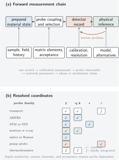
The forward chain runs from a prepared material state to a calibrated record. The inverse arrow is conditional on matrix elements, acceptance, resolution, backgrounds, and nuisance parameters. Different probe families resolve different combinations of energy $E$, momentum $\mathbf q$ or $\mathbf k$, position $\mathbf r$, and delay $t$.

Response, Spectroscopy, Imaging, and Thermodynamics

These categories overlap, but they ask different questions.

Response measurements

A response experiment applies a controlled source $f$ coupled to an operator $B$ through $H_{\mathrm{pert}}(t)=-f(t)B$ and records the change of an observable $A$. Linear response gives

$$\begin{aligned} \delta\langle A(t)\rangle ={}& \int dt'\, \chi_{AB}^{R}(t,t') f(t') \\ & +O(f^2). \end{aligned}$$

Transport, magnetic susceptibility, dielectric response, and many optical measurements fit this pattern. The object inferred is a protocol-dependent response coefficient. The source amplitude must be small enough for linearity, the relevant order of limits must be stated, and heating or hysteresis must be checked.

A dc resistance is not a Hamiltonian eigenvalue. It depends on geometry, contacts, dissipation, current paths, and the limit $\omega\to0$. A static susceptibility likewise depends on whether the field is applied before or after the thermodynamic limit and on demagnetization fields in a finite sample.

Spectroscopy

Spectroscopy resolves energy transferred to or from a material. In a weak-probe description, a transition rate contains an operator matrix element and an energy-conservation kernel:

$$\begin{aligned} \Gamma_{i\to f} \propto{}& \left| \langle f\lvert O_{\mathrm{probe}}\rvert i\rangle \right|^2 \\ & \times \delta(E_f-E_i-\hbar\omega). \end{aligned}$$

After summing over occupied initial states and accepted final states, one obtains a spectral function, structure factor, susceptibility, or a more complicated cross section. Spectral peak positions reveal allowed energy differences only when matrix elements give them weight. Peak widths can combine intrinsic lifetime, inhomogeneity, finite observation time, and instrument resolution.

Angle-resolved photoemission, tunneling spectroscopy, neutron and x-ray energy-loss measurements, Raman scattering, and infrared absorption are spectroscopies, but they do not measure one universal “density of states.” Their coupling operators and final states differ.

Imaging and mapping

An image assigns a measured signal to positions, pixels, scan coordinates, or reconstructed real-space voxels. The displayed contrast need not be a literal map of atomic height or charge density. For example:

• constant-current STM topography mixes geometric height with an energy-integrated tunneling signal;
• magnetic-force and scanning-SQUID images are convolutions with a tip or pickup-loop response;
• coherent diffraction images require phase retrieval;
• spectroscopic maps inherit both spatial and energy resolution;
• domain contrast can depend on polarization, scan direction, and surface termination.

An image should therefore be accompanied by a point-spread function, pixel size, field of view, drift treatment, color scale, and the forward model that assigns contrast to a material quantity.

Thermodynamic and integrated measurements

Heat capacity, magnetization, thermal expansion, and bulk susceptibility usually integrate over momentum and often over many excitation channels. They provide strong evidence for bulk phase transitions and entropy accounting because they do not require a particular surface termination or momentum assignment.

Integration is both a strength and a limitation. A heat-capacity anomaly can establish a bulk thermodynamic event without uniquely identifying its microscopic order. Conversely, a sharp spectroscopic mode can identify an excitation without proving that the entire sample enters a thermodynamic phase. The two kinds of evidence are complementary.

Resolution in Four Coordinates

Resolution describes how sharply the apparatus distinguishes nearby values. It must be quoted together with its definition: standard deviation, full width at half maximum, bin width, Rayleigh criterion, or another convention.

Energy resolution

If an intrinsic line $S(E)$ is measured with a normalized energy-resolution kernel $R_E$, then

$$I_{\mathrm{meas}}(E) = \int dE'\, R_E(E-E') S(E').$$

For Gaussian intrinsic and instrumental profiles with standard deviations $\sigma_{\mathrm{int}}$ and $\sigma_{\mathrm{res}}$,

$$\sigma_{\mathrm{meas}}^2 = \sigma_{\mathrm{int}}^2 + \sigma_{\mathrm{res}}^2.$$

This quadrature rule is not valid for arbitrary line shapes. Lorentzian widths add linearly under convolution, and mixed Gaussian–Lorentzian profiles require a Voigt or more physical model. Blind numerical deconvolution can amplify noise and create artificial substructure.

Momentum resolution

Diffraction and inelastic scattering infer momentum transfer from beam energy and angles. ARPES infers crystal momentum components from photoelectron energy and direction, with a model-dependent treatment of the surface-normal component. Momentum resolution receives contributions from angular divergence, beam bandwidth, sample mosaic, finite illuminated area, and detector pixels.

A finite real-space correlation length $\xi$ broadens a reciprocal-space peak on a scale of order

$$\Delta q \sim \xi^{-1},$$

but the numerical coefficient depends on dimensionality, correlation function, scan direction, and width convention. Instrumental broadening must be separated before assigning $\xi$.

Spatial resolution

Spatial resolution is set by more than pixel spacing. It includes the probe spot, tip shape, interaction volume, diffusion during acquisition, drift, vibration, and reconstruction algorithm. Sampling a field on a $1\,\mathrm{nm}$ grid does not imply $1\,\mathrm{nm}$ physical resolution if the point-spread function is $20\,\mathrm{nm}$ wide.

Local probes trade field of view, acquisition time, perturbation strength, and signal-to-noise against resolution. Atomic contrast on one surface does not by itself establish bulk uniformity.

Time resolution

In pump–probe measurements, the effective time resolution is often the cross-correlation of pump and probe envelopes plus timing jitter and detector response. A short pulse has a broad Fourier bandwidth. For a transform-limited Gaussian pulse, temporal and spectral widths obey a pulse-shape-specific time–bandwidth product; this is not a universal claim that every energy measurement disturbs a sample for $\hbar/\Delta E$.

The relevant question is whether the apparatus can separate the material timescales of interest: electronic redistribution, dephasing, phonon motion, thermalization, domain evolution, and heat diffusion.

Resolution, range, and sensitivity are different

An instrument can have fine resolution but poor sensitivity, a narrow dynamic range, or incomplete phase-space coverage. Reports should distinguish:

• resolution: separation of nearby features;
• accuracy: agreement with a calibrated reference under stated conditions;
• precision: repeatability of the record;
• sensitivity: change in record per change in measurand;
• detection limit: smallest signal distinguishable under a decision rule;
• range and acceptance: values and channels the apparatus can record.

High precision cannot correct an inaccurate calibration, and high energy resolution does not recover excitations forbidden by the probe matrix element.

Bulk and Surface Probes

Every probe has a depth-weighting kernel

A measured signal from depth-dependent material response $s(z)$ can be written

$$I_{\mathrm{meas}} = \int_0^\infty dz\, W(z)s(z).$$

For a simple attenuation model,

$$W(z) = \frac{1}{\lambda} e^{-z/\lambda},$$

where $\lambda$ is an effective information depth. Real kernels depend on incidence and exit angles, energy, material composition, elastic scattering, and geometry.

Photoemission and STM are strongly surface sensitive. Soft and hard x rays, electrons, ions, neutrons, optical fields, and magnetic probes sample different depths and volumes. “Bulk sensitive” never means uniform sensitivity to an infinite depth; it means that the weighting reaches sufficiently far into the sample for the stated inference.

The surface is a different physical system

A cleaved or grown surface can reconstruct, change stoichiometry, bend bands, accumulate charge, adsorb contaminants, host different domains, or break a protecting symmetry. These changes can be scientifically central rather than mere imperfections.

To compare surface and bulk probes:

1. document surface preparation and elapsed time;
2. vary photon energy, incidence angle, tip condition, or another depth-sensitive control;
3. compare several cleaves, positions, and batches;
4. use bulk-sensitive diffraction, thermodynamics, or transport where appropriate;
5. model how a surface state, accumulation layer, or reconstruction contributes to each signal.

Agreement across depth sensitivities is powerful. Disagreement is diagnostic and should not be averaged away.

Equilibrium and Nonequilibrium Probes

Equilibrium is a preparation statement

An equilibrium measurement requires the sample to be stationary on the acquisition timescale and characterized by controlled thermodynamic variables. The probe may still cause transitions, but its backaction should be weak enough that the unperturbed state remains a valid reference for the analysis.

In thermal equilibrium, correlation and response functions are linked by fluctuation–dissipation relations. Under one common convention,

$$S_{AB}(\omega) \propto \frac{ -\operatorname{Im}\chi_{AB}^{R}(\omega) }{ 1-e^{-\beta\hbar\omega} }.$$

The proportionality and sign depend on operator and Fourier conventions; Fluctuation–Dissipation Theorem owns the precise forms. Testing detailed balance can help diagnose thermal equilibrium.

Sweeps can leave equilibrium

Field, temperature, gate, pressure, or current sweeps may encounter slow relaxation, metastability, domain pinning, eddy-current heating, thermal lag, or first-order hysteresis. A trace acquired at a nominal control value can retain memory of the path used to reach it.

Useful checks include:

• reverse the sweep direction;
• vary the sweep rate and dwell time;
• compare field-cooled and zero-field-cooled protocols;
• monitor thermometer and sample-stage lag;
• reduce probe current or intensity;
• repeat after thermal or magnetic reset.

Hysteresis is evidence of history dependence. By itself it does not identify ferromagnetism, a first-order phase transition, or any particular microscopic mechanism.

Pump–probe measurements are two-time experiments

A pump prepares a nonequilibrium state; a delayed probe samples its evolution. The signal is generally a functional of both times,

$$S_{\mathrm{pp}} = S(t_{\mathrm{probe}},t_{\mathrm{pump}}),$$

or of average time and relative time. Time-translation invariance is lost, so an equilibrium spectrum depending only on one frequency need not exist.

Interpreting a transient signal through an effective temperature or instantaneous band structure requires a timescale argument. Electrons, phonons, spins, and domains can have different distributions and relaxation rates. A pump-induced reduction in an order-sensitive signal may arise from heating, screening, matrix-element changes, dephasing, or a true change of order. Fluence dependence, depth matching, polarization controls, absorbed-energy estimates, and recovery dynamics are therefore part of the claim.

What Common Probes Actually Measure

The following are leading correspondences, not exact identities. Every entry is modified by matrix elements, geometry, acceptance, and resolution.

• dc transport. The primary records are voltages and currents. Geometry and a low-frequency device model convert them into resistance or conductivity tensors. Contacts, inhomogeneous current paths, heating, and current jetting are central cautions.
• Hall measurement. The record is a transverse voltage under field or magnetization reversal. Antisymmetrization and geometry lead to Hall resistivity or conductivity. Longitudinal pickup, multiband transport, anomalous Hall terms, and hysteresis can complicate carrier-density inference.
• Quantum oscillations. Oscillatory resistance, torque, or magnetization versus $1/B$ constrains extremal orbit areas and damping factors of mobile carriers. Finite field windows, harmonics, Zeeman splitting, magnetic breakdown, and background subtraction affect the result.
• ARPES. Photoelectron counts versus energy and angle give a matrix-element- and occupation-weighted removal spectrum with surface weighting and momentum resolution. Final states, $k_z$ assignment, charging, surface aging, and matrix-element zeros matter.
• STM and STS. Current and differential conductance versus position and bias approximate a tunneling-weighted local spectral density at the topmost surface. Tip states, setpoint, barrier shape, drift, and surface reconstruction enter the forward model.
• Neutron scattering. Counts versus momentum and energy transfer probe nuclear and magnetic structure factors in the bulk. Form factors, polarization, multiple scattering, sample volume, resolution, and background must be included.
• X-ray scattering. Photon counts versus momentum, energy, and polarization encode charge, lattice, orbital, or resonant cross sections with energy- and geometry-dependent depth sensitivity. Absorption, fluorescence, self-absorption, domains, and the resonance model are common complications.
• Raman, infrared, and THz methods. Intensity or electric-field amplitude and phase versus frequency constrain Raman susceptibilities, dielectric functions, or optical conductivities near zero photon momentum and over a finite penetration depth. Selection rules, extrapolation, substrates, phonons, and heating matter.
• Thermodynamics and magnetometry. Heat flow, temperature, force, torque, or magnetic moment lead to heat capacity, entropy changes, magnetization, or susceptibility integrated over sample volume. Addenda, demagnetization, impurity tails, subtraction, and equilibration set important systematics.
• Pump–probe methods. Delay-dependent optical, photoemission, or diffraction changes sample a nonequilibrium response or correlation snapshot with finite time and depth weighting. Coherent artifacts, fluence, depth mismatch, heating, and nonthermal distributions constrain interpretation.

Transport is weighted toward long-lived mobile channels

Conductivity emphasizes states and scattering processes that carry current. A small, high-mobility band can dominate transport while containing a minority of carriers. Contact resistance can dominate a two-terminal device, and anisotropic samples can distort current paths. Transport is therefore not a direct density-of-states measurement.

Spectroscopy is operator selective

ARPES inserts an electron-removal operator and observes an outgoing electron after photoexcitation. Neutron spin scattering couples to magnetization components transverse to momentum transfer, weighted by magnetic form factors and polarization geometry. Raman scattering selects symmetry channels through photon polarizations. A missing peak may mean absence, weak matrix element, wrong polarization, inaccessible momentum, or insufficient sensitivity.

Thermodynamics counts states without locating them

At low temperature, electronic heat capacity can constrain a density of low-energy states, while entropy integration tests how much spectral weight participates in a transition. Magnetization and susceptibility constrain net moments and field response. These are bulk-integrated quantities: they can test whether a spectroscopic feature is representative, but they rarely reveal its full momentum structure.

From Several Probes to One Claim

Orthogonality is more valuable than repetition

Independent evidence should fail for different reasons. For a proposed bulk gap:

• transport can show activated conduction but is vulnerable to parallel channels;
• optical spectroscopy can constrain absorption onset and residual conductivity;
• tunneling can map a local single-particle suppression but is surface sensitive;
• heat capacity can test for residual bulk low-energy states;
• diffraction can detect a structural transition that offers an alternative mechanism.

Five spectra taken with the same surface-sensitive matrix element are less independent than one surface spectrum, one bulk thermodynamic measurement, and one structural control.

A phase claim needs scale, symmetry, and reproducibility

A defensible phase assignment normally combines:

1. a stated symmetry or topological distinction;
2. a bulk or finite-size criterion appropriate to that distinction;
3. characteristic excitations or response;
4. control-parameter evolution and limiting cases;
5. exclusion of plausible structural, magnetic, contact, and heating artifacts;
6. repeatability across positions and samples;
7. consistency among probes with different couplings and depths.

No single checklist is universal. A superconducting phase, density wave, topological band structure, and spin liquid demand different decisive evidence. The Quantum Matter Map organizes those phase-specific ledgers.

Reporting and Uncertainty

Keep raw, corrected, and inferred quantities separate

A figure should make clear whether it shows:

• unprocessed counts or digitizer output;
• calibrated but uncorrected data;
• background-subtracted or normalized data;
• deconvolved or symmetrized data;
• a fitted model component;
• an inferred physical parameter.

Preserve the transformation chain and code. A smooth published curve without the raw record can conceal dead pixels, masked regions, drift corrections, normalization choices, or unstable fits.

Uncertainty follows the measurement model

If an inferred quantity $y=g(\mathbf x)$ depends on inputs $x_i$ with covariance matrix $\Sigma$, first-order propagation gives

$$u_y^2 \approx \sum_{i,j} \frac{\partial g}{\partial x_i} \Sigma_{ij} \frac{\partial g}{\partial x_j}.$$

This includes correlated calibration and nuisance inputs. Counting statistics alone are rarely the complete uncertainty. Model discrepancy, sample variation, background choice, and non-identifiability may require sensitivity intervals, alternative models, hierarchical analysis, or explicit qualitative limitations rather than one standard error.

Report confidence or credible intervals with their construction and coverage meaning. Error bars should not be used as generic decorations, and lack of visible error bars does not imply exact data.

Common Mistakes

• Treating detector intensity as the intrinsic spectral function.
• Calling a conductance minimum a bulk energy gap without geometry and parallel-channel checks.
• Inferring absence of an excitation from a matrix-element-suppressed spectrum.
• Quoting pixel spacing, angular bin width, or pulse duration as the full physical resolution.
• Deconvolving weak data without regularization tests or reconvolution residuals.
• Assigning a reciprocal-space peak width entirely to correlation length before subtracting instrument and mosaic broadening.
• Generalizing one clean surface region to the sample bulk.
• Combining repeated processing of one dataset as independent confirmation.
• Using equilibrium response formulas after a strong pump without a timescale argument.
• Calling hysteresis proof of one particular ordered phase.
• Fitting one model without showing whether plausible alternatives are distinguishable.
• Reporting statistical fit errors while omitting calibration, background, sample, and model uncertainty.

Exercises

1. Separate instrumental and intrinsic width

A Gaussian spectral peak has measured full width at half maximum $18\,\mathrm{meV}$. The independently calibrated Gaussian energy resolution is $12\,\mathrm{meV}$ FWHM. Estimate the intrinsic FWHM.

Solution

For Gaussian profiles, variances add under convolution. Because FWHM is proportional to the standard deviation by the same factor for every Gaussian, the squared FWHM values also add:

$$\begin{aligned} w_{\mathrm{int}} &= \sqrt{ w_{\mathrm{meas}}^2 - w_{\mathrm{res}}^2 } \\ &= \sqrt{ (18\,\mathrm{meV})^2 - (12\,\mathrm{meV})^2 } \\ &\simeq 13.4\,\mathrm{meV}. \end{aligned}$$

This estimate is valid only if both line shapes are well described by Gaussians and the resolution calibration applies to the same settings. A Lorentzian intrinsic line convolved with a Gaussian instrument response requires a Voigt analysis.

2. Quantify surface weighting

For $W(z)=\lambda^{-1}e^{-z/\lambda}$, what fraction of the signal originates within the first $2\lambda$ of the surface?

Solution

The fraction is

$$\begin{aligned} F(2\lambda) &= \int_0^{2\lambda} \frac{dz}{\lambda} e^{-z/\lambda} \\ &= 1-e^{-2} \simeq 0.865. \end{aligned}$$

About $86.5\%$ of the signal comes from that depth in the ideal exponential model. The remaining contribution is not zero, and a real information-depth kernel may differ because of incidence angle, elastic scattering, and material-specific attenuation.

3. Diagnose a missing spectroscopic peak

A calculated excitation at $(\mathbf q_0,\omega_0)$ is absent from one polarization channel of a scattering experiment. Give four explanations that do not require the excitation itself to be absent, and propose a discriminating test.

Solution

Possible explanations include:

1. a symmetry or polarization selection rule makes the matrix element vanish;
2. $\mathbf q_0$ lies outside the instrument acceptance or is misassigned;
3. the mode is broader than the sensitivity permits because of intrinsic decay or inhomogeneity;
4. background, absorption, or resolution obscures the feature.

Change polarization or sample orientation while keeping the target point accessible, map neighboring momenta, and measure a reference mode with known symmetry. A genuine matrix-element zero should follow the predicted geometry, whereas an absent state remains absent in every channel that should couple to it.

4. Identify a non-identifiable inversion

A measured line is fitted equally well by two narrow intrinsic peaks convolved with the calibrated resolution and by one broader asymmetric intrinsic peak. What can be concluded, and what measurement would help?

Solution

The current data establish spectral weight over the observed energy interval but do not identify whether the intrinsic response has one component or two. Reporting the two-peak separation as a resolved splitting would exceed the information in the record.

Useful additions include a measurement with substantially narrower and independently calibrated resolution, a polarization or momentum setting that changes the two proposed components differently, or a second probe with different matrix elements. Both models should be reconvolved and compared to held-out data rather than judged only by their best fit to the original trace.

5. Test an equilibrium assumption

A resistance anomaly shifts when the temperature sweep is accelerated and differs between warming and cooling. List the minimum checks before assigning an equilibrium phase boundary.

Solution

The observations indicate history dependence or thermal lag. At minimum:

1. repeat several sweep rates and extrapolate toward a slow, settled limit;
2. dwell at fixed temperatures while monitoring both sample and stage thermometry;
3. reduce measurement current to test Joule heating;
4. reset the sample through a reproducible thermal protocol;
5. compare multiple contacts and samples;
6. check for simultaneous structural, magnetic, or calorimetric signatures.

An equilibrium boundary should be quoted only after the settled result is separated from kinetic hysteresis and thermometer lag. If metastability is intrinsic, both branches and the protocol belong to the result.

6. Build an orthogonal evidence set

A surface-sensitive spectrum shows a gap and an in-gap state consistent with a proposed topological material. Choose three additional measurements that strengthen or falsify the claim, and explain their distinct roles.

Solution

One strong set is:

1. bulk-sensitive spectroscopy or transport: tests whether the chemical potential and bulk gap are appropriate rather than properties of a reconstructed surface;
2. surface-state dispersion under controlled termination or thickness: tests the predicted boundary connectivity and finite-size evolution rather than the mere presence of an in-gap feature;
3. structure, symmetry, and composition characterization: verifies that the crystal and magnetic symmetry assumed by the topological classification are realized.

A fourth useful element is a response tied to the relevant invariant, with trivial bulk, surface, and contact mechanisms explicitly modeled. These measurements are valuable because their dominant systematic errors differ from those of the original surface spectrum.

Research Status

• Established: linear-response theory; scattering kinematics; spectral and structure-factor representations; instrument-resolution convolution; calibrated electrical, optical, thermodynamic, diffraction, photoemission, tunneling, and neutron methods.
• Active: quantitative multimodal data fusion; operando and extreme-environment probes; higher spatial and temporal resolution at controlled perturbation strength; uncertainty-aware inversion; reproducible autonomous acquisition; separating intertwined electronic, spin, orbital, and lattice dynamics.
• Method dependent: deconvolution, background models, phase retrieval, analytic continuation, effective-temperature descriptions, and microscopic parameter extraction. These can be reliable in validated regimes but are not raw observables.
• Speculative when unsupported: identifying a new phase or mechanism from one suggestive feature without probe-specific controls, bulk–surface reconciliation, sample replication, and competing-model tests.

Connections

• Unconventional Superconductivity combines calibrated records from several canonical probes into a bounded pairing-symmetry claim; this page retains the general detector-to-observable-to-claim and uncertainty contract.
• Transport Measurements develops four-terminal wiring, reversal protocols, geometry and tensor conversion, sweep controls, and uncertainty budgets for electrical transport.
• Hall Measurements develops signed transverse-voltage acquisition, field parity, carrier inference, magnetic hysteresis, and quantization checks.
• Quantum Oscillations follows raw field traces through inverse-field spectra, damping fits, orbit reconstruction, and model-dependent phase inference.
• Angle-Resolved Photoemission Spectroscopy follows photoelectron counts through energy–momentum calibration, occupied spectral-function inference, surface and matrix-element controls, and correlation claims.
• Pump–Probe Spectroscopy follows repeated excitation through absorbed-fluence and depth calibration, transient reflectivity, trARPES, coherent phonons, relaxation models, and light-induced-state evidence.
• Heat Capacity and Thermodynamics follows heater and thermometer records through thermal-link models, addenda subtraction, component separation, entropy integration, and bulk-transition claims.
• Magnetic Susceptibility follows SQUID, VSM, and ac records through background, normalization, demagnetization, response decomposition, and magnetic-phase claim controls.
• Vortex Matter, Pinning, and Flux Flow combines transport, magnetic, microwave, and imaging outputs into a bounded claim about entry, pinning, creep, collective order, or driven flux motion while the probe pages retain acquisition and inversion.
• Superconducting Proximity Effect turns calibrated thickness-, temperature-, field-, and spectrum-dependent observations into a bounded claim about bulk anomalous propagation or inverse suppression; this page retains the probe-independent acquisition and inference contract.
• Device Fabrication Concepts follows materials through contacts, gates, assembly, encapsulation, process disorder, cryogenic integration, and batch-level reproducibility.
• Data Interpretation and Pitfalls turns the measurement contract into a cross-probe audit of competing mechanisms, depth, sample variation, contacts, topology, and history dependence.
• Quantum Matter Map organizes phase claims by structure, energy scales, response, and evidence.
• Conventions for Quantum Matter fixes reciprocal-space, spectral, electromagnetic, and response conventions.
• Quantum Matter Reference and Data packages a probe lookup as a convention- and provenance-complete transferable record; this page remains the canonical owner of detector-to-observable forward modeling and experimental inference.
• Kubo Formula derives the source-to-response relation and its contact terms.
• Spectral Functions distinguishes Hamiltonian spectra, operator spectral weight, intrinsic lines, and measured intensity.
• Structure Factors develops static and dynamic density, spin, bond, and pair correlations probed by scattering.
• Susceptibilities supplies source, tensor, unit, and protocol dictionaries.
• What Is a Scattering Experiment? connects incident exposure and detector counts to differential cross sections.
• Convolution supplies the mathematical operation behind resolution broadening.
• Error Estimates develops truncation, discretization, and uncertainty logic for data reduction and models.
• Quantum Materials by Design places property measurement and independent reproduction inside the materials-discovery loop.

Further Reading

• G. L. Squires, Introduction to the Theory of Thermal Neutron Scattering, for the relation among scattering kinematics, nuclear and magnetic couplings, and dynamic correlations.
• A. Damascelli, Z. Hussain, and Z.-X. Shen, “Angle-Resolved Photoemission Studies of the Cuprate Superconductors,” for the route from photoelectron intensity to momentum-resolved removal spectra.
• D. N. Basov et al., “Electrodynamics of Correlated Electron Materials,” for frequency-dependent conductivity, sum rules, and correlated-material interpretation.
• C. Giannetti et al., “Ultrafast Optical Spectroscopy of Strongly Correlated Materials and High-Temperature Superconductors,” for nonequilibrium timescales and caution around light-induced-state language.
• JCGM 100, Guide to the Expression of Uncertainty in Measurement, for a general measurement-model approach to uncertainty.

References

1. R. Kubo, “Statistical-Mechanical Theory of Irreversible Processes. I. General Theory and Simple Applications to Magnetic and Conduction Problems,” Journal of the Physical Society of Japan 12, 570–586 (1957), doi:10.1143/JPSJ.12.570.
2. H. B. Callen and T. A. Welton, “Irreversibility and Generalized Noise,” Physical Review 83, 34–40 (1951), doi:10.1103/PhysRev.83.34.
3. L. Van Hove, “Correlations in Space and Time and Born Approximation Scattering in Systems of Interacting Particles,” Physical Review 95, 249–262 (1954), doi:10.1103/PhysRev.95.249.
4. G. L. Squires, Introduction to the Theory of Thermal Neutron Scattering, 3rd ed. (Cambridge University Press, 2012), doi:10.1017/CBO9781139107808.
5. J. Als-Nielsen and D. McMorrow, Elements of Modern X-Ray Physics, 2nd ed. (Wiley, 2011), doi:10.1002/9781119998365.
6. L. J. P. Ament, M. van Veenendaal, T. P. Devereaux, J. P. Hill, and J. van den Brink, “Resonant Inelastic X-Ray Scattering Studies of Elementary Excitations,” Reviews of Modern Physics 83, 705–767 (2011), doi:10.1103/RevModPhys.83.705.
7. A. Damascelli, Z. Hussain, and Z.-X. Shen, “Angle-Resolved Photoemission Studies of the Cuprate Superconductors,” Reviews of Modern Physics 75, 473–541 (2003), doi:10.1103/RevModPhys.75.473.
8. J. Tersoff and D. R. Hamann, “Theory of the Scanning Tunneling Microscope,” Physical Review B 31, 805–813 (1985), doi:10.1103/PhysRevB.31.805.
9. J. Bardeen, “Tunnelling from a Many-Particle Point of View,” Physical Review Letters 6, 57–59 (1961), doi:10.1103/PhysRevLett.6.57.
10. D. N. Basov, R. D. Averitt, D. van der Marel, M. Dressel, and K. Haule, “Electrodynamics of Correlated Electron Materials,” Reviews of Modern Physics 83, 471–541 (2011), doi:10.1103/RevModPhys.83.471.
11. M. Dressel and G. Grüner, Electrodynamics of Solids (Cambridge University Press, 2002), doi:10.1017/CBO9780511606168.
12. D. Shoenberg, Magnetic Oscillations in Metals (Cambridge University Press, 1984), doi:10.1017/CBO9780511897870.
13. C. Giannetti et al., “Ultrafast Optical Spectroscopy of Strongly Correlated Materials and High-Temperature Superconductors: A Non-Equilibrium Approach,” Advances in Physics 65, 58–238 (2016), doi:10.1080/00018732.2016.1194044.
14. P. R. Bevington and D. K. Robinson, Data Reduction and Error Analysis for the Physical Sciences, 3rd ed. (McGraw-Hill, 2003).
15. Joint Committee for Guides in Metrology, Evaluation of Measurement Data—Guide to the Expression of Uncertainty in Measurement, JCGM 100:2008 (2008), doi:10.59161/JCGM100-2008E.

Summary

Quantum-matter experiments measure detector records through finite, selective apparatuses. Response measurements infer source-dependent coefficients; spectroscopy resolves operator-weighted transitions; imaging maps a convolved contrast; thermodynamics integrates bulk states. Energy, momentum, position, and time resolution must be distinguished from sensitivity, accuracy, range, and acceptance. Surface and bulk probes weight different physical systems, while pump–probe methods generally require two-time nonequilibrium models. Trust comes from an explicit forward model, preserved reduction chain, complete uncertainty budget, orthogonal probes, and claims that stop at the highest evidence rung actually reached.