Measurement in the Formalism

In the standard formalism, a quantum measurement is a rule that connects an input state to:

1. a probability distribution over recorded outcomes;
2. a conditional output state for each outcome that can occur.

The first item predicts classical data. The second item supplies the state used for later predictions after the record is known. Together they form the operational measurement model.

The scope is deliberately limited:

• measurement formalism means the mathematical probability-and-update rules;
• detector physics means a dynamical model of coupling, amplification, noise, timing, and readout;
• the measurement problem asks how definite macroscopic outcomes and the quantum state should be understood physically.

This page develops the first layer. A detector model can justify or approximate particular operators, and interpretations disagree about the physical status of state update, but neither issue changes how the stated operational model is used to calculate probabilities.

Measurement as an Input–Output Rule

Begin with an input density operator

$$\rho\ge0, \qquad \operatorname{Tr}\rho=1.$$

A discrete measurement has an outcome set

$$\Omega = \lbrace x_1,x_2,\ldots\rbrace.$$

For each input state, the model must provide probabilities obeying

$$p(x)\ge0, \qquad \sum_{x\in\Omega}p(x)=1.$$

If outcome $x$ is retained, the model may also provide a normalized conditional state $\rho_x$. The pair

$$\bigl(p(x),\rho_x\bigr)$$

is what a later experiment needs: the probability of reaching that branch and the state from which subsequent predictions begin.

For a pure input, one may write

$$\rho = \lvert\psi\rangle\langle\psi\rvert,$$

but density operators are the natural language because selective and nonselective measurements can produce mixed ensembles even when the input was pure.

Three Layers That Must Not Be Collapsed

A measurement description can contain three mathematically distinct layers.

Outcome labels

The symbols $x$ are classical records: numbers, detector clicks, pointer positions, bit strings, or coarse-grained categories. Their numerical labels alone do not determine quantum probabilities.

Probability operators

Positive operators $E_x$ assign outcome probabilities through

$$p(x) = \operatorname{Tr}(\rho E_x).$$

For a projective measurement, the $E_x$ are orthogonal projectors. More generally, they form a POVM.

State-changing operations

A quantum operation $\mathcal I_x$ assigns the unnormalized output branch

$$\mathcal I_x(\rho).$$

Its trace is the outcome probability,

$$p(x) = \operatorname{Tr}\mathcal I_x(\rho),$$

and, when $p(x)>0$, the conditional state is

$$\rho_x = \frac{\mathcal I_x(\rho)}{p(x)}.$$

The family $\lbrace\mathcal I_x\rbrace$ is a quantum instrument. The effects $E_x$ determine probabilities, while the instrument contains the additional state-update information. Two instruments can have the same effects and the same outcome statistics but different conditional output states.

The instrument language is the most general of these three. The ideal projective model is the central special case and the right place to begin.

Ideal Sharp Measurements

For a discrete ideal sharp measurement, outcomes $a$ are represented by an orthogonal family of projectors:

$$P_a^\dagger=P_a, \qquad P_a^2=P_a,$$ $$P_aP_b = \delta_{ab}P_a, \qquad \sum_aP_a=I.$$

If the measurement is described by a self-adjoint observable,

$$A = \sum_a aP_a,$$

then $a$ is the recorded value and $P_a$ projects onto the full eigenspace with that eigenvalue.

The projector is the essential probability object. If $a$ is degenerate, $P_a$ has rank greater than one. The number $a$ does not select a preferred basis inside that eigenspace.

The spectral and joint-measurement structure is developed in Projective Measurement.

Outcome Probabilities

For a pure state,

$$p(a) = \langle\psi|P_a|\psi\rangle = \lVert P_a\lvert\psi\rangle\rVert^2.$$

For a density operator,

$$p(a) = \operatorname{Tr}(\rho P_a).$$

Positivity follows because $P_a$ is positive. Normalization follows from the resolution of the identity:

$$\begin{aligned} \sum_a p(a) &= \sum_a\operatorname{Tr}(\rho P_a) \\ &= \operatorname{Tr} \left( \rho\sum_aP_a \right) \\ &= \operatorname{Tr}\rho = 1. \end{aligned}$$

These are instances of the Born Rule. The rule predicts frequencies for repeated preparations and probabilities for individual outcomes according to the adopted probabilistic interpretation. It does not replace the outcome set or the state-update model.

Expectation values are recovered from the same distribution:

$$\langle A\rangle_\rho = \sum_a a\,p(a) = \operatorname{Tr}(\rho A).$$

Selective State Update

Suppose outcome $a$ is actually recorded and $p(a)>0$. The ideal Lüders branch is

$$\mathcal I_a(\rho) = P_a\rho P_a.$$

Its trace is

$$\operatorname{Tr}\mathcal I_a(\rho) = \operatorname{Tr}(\rho P_a) = p(a).$$

The normalized selective update is therefore

$$\rho \longmapsto \rho_a = \frac{P_a\rho P_a} {\operatorname{Tr}(\rho P_a)}.$$

For a pure input, this reduces to

$$\lvert\psi\rangle \longmapsto \lvert\psi_a\rangle = \frac{P_a\lvert\psi\rangle} {\sqrt{\langle\psi|P_a|\psi\rangle}}.$$

The denominator is not optional. $P_a\lvert\psi\rangle$ has squared norm $p(a)$, so normalization conditions on the selected branch divide by that probability.

If $p(a)=0$, the conditional state is undefined because that branch never occurs in the stated model. Assigning an arbitrary normalized vector to a zero-probability branch has no operational content.

The update is a conditional rule for future predictions. It should be applied only after specifying which outcome was retained. Its dedicated treatment is State Update Rule.

Nonselective State Update

Suppose the measurement interaction occurs but the outcome is not available, is discarded, or is averaged over. The appropriate output is the weighted mixture of conditional branches:

$$\rho' = \sum_a p(a)\rho_a.$$

For the ideal projective instrument,

$$\rho' = \sum_aP_a\rho P_a.$$

This map is trace preserving:

$$\begin{aligned} \operatorname{Tr}\rho' &= \sum_a\operatorname{Tr}(P_a\rho P_a) \\ &= \operatorname{Tr} \left( \rho\sum_aP_a \right) \\ &=1. \end{aligned}$$

It removes coherence between different outcome subspaces while preserving coherence within each degenerate subspace.

Forgetting an outcome is not the same physical operation as never performing the measurement. If no measurement occurs, the state remains $\rho$ apart from ordinary dynamics. If a measurement occurs and its record is ignored, the system is generally described by $\sum_aP_a\rho P_a$.

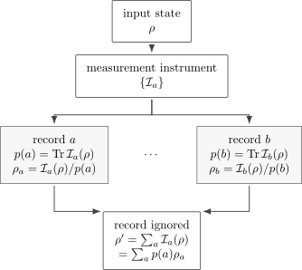
A quantum instrument maps the input $\rho$ to unnormalized branches $\mathcal I_a(\rho)$. Retaining outcome $a$ gives the conditional state $\rho_a=\mathcal I_a(\rho)/p(a)$; ignoring the record gives the nonselective state $\rho'=\sum_a\mathcal I_a(\rho)=\sum_a p(a)\rho_a$.

Repeatability and Its Limits

The ideal sharp update is repeatable in a narrow mathematical sense. Since

$$P_a\rho_aP_a = \rho_a,$$

an immediate repetition of the same projective measurement gives

$$\Pr(a\text{ again}\mid a) = \operatorname{Tr}(\rho_aP_a) = 1.$$

This statement assumes:

• the same projective measurement is repeated;
• no intervening unitary dynamics, noise, or coupling changes the state;
• the first measurement realizes the ideal Lüders instrument.

Repeatability is not a universal property of measurement. Generalized, continuous, destructive, weak, or noisy measurements can fail it. A detector that absorbs a photon can report its energy accurately without leaving the same photon available for a repeated measurement.

Repeatability also does not mean that every basis vector inside a degenerate eigenspace is preserved by every apparatus measuring the same coarse outcome. The Lüders instrument is a particular minimally refining idealization.

Qubit Example: Measuring Along z

Write a qubit state in Bloch form:

$$\rho = \frac12 \left( I + r_x\sigma_x + r_y\sigma_y + r_z\sigma_z \right),$$

where

$$r_x^2+r_y^2+r_z^2\le1.$$

The sharp $z$-measurement projectors are

$$P_\pm = \frac12(I\pm\sigma_z).$$

The outcome probabilities are

$$p(\pm) = \operatorname{Tr}(\rho P_\pm) = \frac{1\pm r_z}{2}.$$

Because the projectors have rank one, the conditional states are

$$\rho_\pm=P_\pm$$

whenever the corresponding probability is nonzero.

If the outcome is ignored,

$$\begin{aligned} \rho' &= P_+\rho P_+ + P_-\rho P_- \\ &= \frac12 \left( I+r_z\sigma_z \right). \end{aligned}$$

The $x$ and $y$ Bloch components vanish. These components encoded coherence between the two $z$-outcome subspaces. The population difference $r_z$ remains.

For the pure state

$$\lvert\psi\rangle = \alpha\lvert0\rangle + \beta\lvert1\rangle, \qquad |\alpha|^2+|\beta|^2=1,$$

the same formulas give

$$p(+)=|\alpha|^2, \qquad p(-)=|\beta|^2.$$

Degenerate Outcome Example

Consider a three-level system and the two projectors

$$P_0 = \lvert0\rangle\langle0\rvert + \lvert1\rangle\langle1\rvert,$$ $$P_1 = \lvert2\rangle\langle2\rvert.$$

For

$$\lvert\psi\rangle = \alpha\lvert0\rangle + \beta\lvert1\rangle + \gamma\lvert2\rangle,$$

the probability of the degenerate outcome $0$ is

$$p(0) = |\alpha|^2+|\beta|^2.$$

If it occurs and $p(0)>0$, the Lüders state is

$$\lvert\psi_0\rangle = \frac{ \alpha\lvert0\rangle+\beta\lvert1\rangle } {\sqrt{|\alpha|^2+|\beta|^2}}.$$

The relative phase and coherence between $\lvert0\rangle$ and $\lvert1\rangle$ survive. The measurement distinguishes the subspace $\operatorname{Ran}P_0$ from $\operatorname{Ran}P_1$; it does not secretly measure which basis vector inside $P_0$ was present.

An apparatus that further distinguishes $\lvert0\rangle$ from $\lvert1\rangle$ realizes a finer measurement. Degenerate state update and the difference between Lüders and finer von Neumann refinements belong to Degenerate Measurements and Lüders Rule.

Sequential Measurements Preview

State update matters because it changes later probabilities. For projectors $P_a$ followed by $Q_b$, the joint ordered probability is

$$\begin{aligned} p(a\text{ then }b) &= p(a)\, \operatorname{Tr}(\rho_aQ_b) \\ &= \operatorname{Tr} \left( Q_bP_a\rho P_a \right). \end{aligned}$$

For a pure input,

$$p(a\text{ then }b) = \lVert Q_bP_a\lvert\psi\rangle\rVert^2.$$

Reversing the order generally replaces $Q_bP_a$ by $P_aQ_b$ and changes the probability tree. If all relevant projectors commute, the ideal sequential probabilities reduce to a common joint distribution and the order does not matter.

The complete conditional-probability calculus and order effects belong to Sequential Measurements.

Measurement in a Chosen Basis

Given an orthonormal basis $\lbrace\lvert n\rangle\rbrace$, the associated rank-one projectors are

$$P_n = \lvert n\rangle\langle n\rvert.$$

If

$$\lvert\psi\rangle = \sum_n c_n\lvert n\rangle,$$

then

$$p(n) = |c_n|^2 = |\langle n|\psi\rangle|^2.$$

The selective ideal output is the ray represented by $\lvert n\rangle$. A change of measurement basis changes the projectors and therefore changes both the amplitudes and probabilities. The practical coefficient calculations live in Measurement in a Chosen Basis.

Generalized Measurements Preview

Projective measurements are not the full operational language. A discrete generalized instrument can be written using measurement operators $M_{x\alpha}$:

$$\mathcal I_x(\rho) = \sum_\alpha M_{x\alpha}\rho M_{x\alpha}^\dagger.$$

Normalization of the full measurement requires

$$\sum_{x,\alpha} M_{x\alpha}^\dagger M_{x\alpha} = I.$$

The effect for outcome $x$ is

$$E_x = \sum_\alpha M_{x\alpha}^\dagger M_{x\alpha},$$

so

$$p(x) = \operatorname{Tr}(\rho E_x).$$

The effects obey

$$E_x\ge0, \qquad \sum_xE_x=I,$$

and therefore form a POVM.

This framework describes noisy discrimination, inefficient detection, coarse-grained records, weak readout, indirect ancilla measurements, and many other procedures. Generalized Measurements Overview develops the operators and update rules; POVMs: First Encounter develops the probability-only effect language.

The Same POVM Can Have Different Updates

Consider the computational-basis effects

$$E_0 = \lvert0\rangle\langle0\rvert, \qquad E_1 = \lvert1\rangle\langle1\rvert.$$

The Lüders measurement operators

$$M_0=E_0, \qquad M_1=E_1$$

produce the familiar conditional basis states.

Now let

$$N_0 = \lvert+\rangle\langle0\rvert, \qquad N_1 = \lvert+\rangle\langle1\rvert,$$

where

$$\lvert+\rangle = \frac{\lvert0\rangle+\lvert1\rangle}{\sqrt2}.$$

The effects are unchanged:

$$N_0^\dagger N_0=E_0, \qquad N_1^\dagger N_1=E_1.$$

Thus both instruments give the same outcome probabilities for every input state. But the second instrument resets the system to $\lvert+\rangle$ after either outcome.

A POVM tells us what classical outcome statistics to expect. It does not, by itself, determine the post-measurement state.

Classical Record and Quantum Output

A measurement has both a classical output and, when the system remains available, a quantum output. Introduce orthonormal record states $\lvert x\rangle_X$. The joint classical–quantum output can be represented as

$$\rho_{XQ}' = \sum_x \lvert x\rangle\langle x\rvert_X \otimes \mathcal I_x(\rho).$$

The trace of the $x$ block is $p(x)$. Reading the classical register and conditioning on $x$ gives $\rho_x$. Ignoring the register gives the nonselective quantum output

$$\rho_Q' = \sum_x\mathcal I_x(\rho).$$

This representation makes selective and nonselective descriptions two views of one instrument rather than competing update rules.

Calibration and Detector Physics

The formal operators are not labels attached to an apparatus by declaration. A physical measurement model requires a calibration statement connecting records to effects or instruments. Experimentally, that connection can be tested using known preparations, tomography, control experiments, and uncertainty estimates.

Different devices can realize the same ideal projectors or POVM effects while differing in:

• efficiency and dark counts;
• time resolution and dead time;
• destructive versus nondestructive readout;
• post-measurement disturbance;
• coupling strength and bandwidth;
• unrecorded environmental channels.

Those differences matter whenever later system dynamics or sequential measurements are predicted. The abstract formalism begins after an effective instrument has been specified; deriving it from a system–apparatus Hamiltonian is additional physics.

What the Formalism Does Not Settle

The probability-and-update calculus does not, by itself, answer:

• why an individual run has one definite macroscopic record;
• whether conditional state update is a physical collapse, an information update, an effective description, or a branch-relative statement;
• how microscopic alternatives become robust macroscopic records;
• which interpretation of quantum mechanics is correct;
• where, if anywhere, a fundamental system–apparatus boundary lies.

Decoherence explains how environmental entanglement suppresses interference between selected reduced-state sectors and stabilizes records under suitable conditions. It does not, without further interpretive assumptions, select one unique outcome from the global state.

These issues are separated carefully in What Measurement Formalism Does Not Settle.

A Reliable Calculation Workflow

For a measurement problem:

1. Write the input state. Use a normalized ket or density operator.
2. Identify the outcome data. Specify projectors, effects, or the full instrument, not only numerical labels.
3. Compute probabilities. Use $p(x)=\operatorname{Tr}\mathcal I_x(\rho) =\operatorname{Tr}(\rho E_x)$.
4. Condition only on an obtained outcome. Divide the branch operation by its nonzero probability.
5. Average if the record is unavailable. Sum the unnormalized branches.
6. Use the output state for later steps. Apply subsequent dynamics and measurements to $\rho_x$ or to the nonselective $\rho'$ as appropriate.
7. State the idealizations. Note whether the model assumes projectivity, repeatability, perfect efficiency, no intervening dynamics, or a specific detector instrument.

This order keeps normalization, conditioning, and physical assumptions visible.

Common Mistakes

• Treating outcome numbers as sufficient measurement data without projectors, effects, or an instrument.
• Using $p(a)=\langle\psi|A|\psi\rangle$; this is an expectation value, not the probability of eigenvalue $a$.
• Applying a selective update without naming the outcome that occurred.
• Dividing by a zero outcome probability.
• Confusing an unread measurement with no measurement.
• Erasing coherence inside a degenerate eigenspace when the Lüders projector preserves it.
• Assuming every POVM specifies a unique post-measurement state.
• Assuming repeatability for noisy, destructive, weak, or continuous measurements.
• Reusing the pre-measurement state in a sequential calculation after a selective outcome.
• Treating the operational rules as a complete microscopic detector model or as a settled interpretation of quantum mechanics.

Canonical Boundaries

• Born Rule owns the probability postulate and its discrete, continuous, and projector forms.
• Projective Measurement owns PVM structure, sharp outcomes, degeneracy, coarse graining, and repeatability assumptions.
• State Update Rule owns the selective and nonselective projective update derivations.
• Degenerate Measurements and Lüders Rule owns preservation within degenerate eigenspaces and finer refinements.
• Sequential Measurements owns ordered probability trees and disturbance.
• Generalized Measurements Overview owns measurement operators and instruments beyond PVMs.
• POVMs: First Encounter owns positive effects and probability-only generalized measurements.
• What Measurement Formalism Does Not Settle owns the boundary with detector physics, decoherence, and interpretation.

Summary

A complete operational measurement model connects an input $\rho$ to both classical outcome probabilities and conditional quantum outputs:

$$p(x) = \operatorname{Tr}\mathcal I_x(\rho), \qquad \rho_x = \frac{\mathcal I_x(\rho)}{p(x)}.$$

For an ideal projective measurement,

$$\mathcal I_a(\rho) = P_a\rho P_a.$$

Retaining outcome $a$ gives the selective Lüders state; ignoring the record gives

$$\rho' = \sum_aP_a\rho P_a.$$

The probability effects do not generally determine the update instrument. Repeatability is a property of a special ideal model, not of all measurements. These formal rules support precise calculations while remaining distinct from detector dynamics and from interpretive questions about definite outcomes.

References

• J. von Neumann, Mathematical Foundations of Quantum Mechanics, Princeton University Press, 1955.
• G. Lüders, “Über die Zustandsänderung durch den Meßprozeß,” Annalen der Physik 8, 322–328, 1951; English translation and discussion, arXiv:quant-ph/0403007.
• E. B. Davies and J. T. Lewis, “An operational approach to quantum probability,” Communications in Mathematical Physics 17, 239–260, 1970, doi:10.1007/BF01647093.
• M. Ozawa, “Quantum measuring processes of continuous observables,” Journal of Mathematical Physics 25, 79–87, 1984, doi:10.1063/1.526000.
• K. Kraus, States, Effects, and Operations, Springer, 1983.
• A. S. Holevo, Probabilistic and Statistical Aspects of Quantum Theory, 2nd ed., Edizioni della Normale, 2011.
• P. Busch, P. J. Lahti, J.-P. Pellonpää, and K. Ylinen, Quantum Measurement, Springer, 2016.
• A. Peres, Quantum Theory: Concepts and Methods, Kluwer, 1995.
• M. A. Nielsen and I. L. Chuang, Quantum Computation and Quantum Information, 10th anniversary ed., Cambridge University Press, 2010.

Exercises

Exercise 1: Normalize projective probabilities

Let $\lbrace P_a\rbrace$ be orthogonal projectors with $\sum_aP_a=I$. Prove that

$$p(a)=\operatorname{Tr}(\rho P_a)$$

is a normalized probability distribution for every density operator $\rho$.

Solution

Since $\rho\ge0$ and $P_a\ge0$,

$$p(a) = \operatorname{Tr} \left( \rho^{1/2}P_a\rho^{1/2} \right) \ge0.$$

Summing gives

$$\begin{aligned} \sum_a p(a) &= \sum_a\operatorname{Tr}(\rho P_a) \\ &= \operatorname{Tr} \left( \rho\sum_aP_a \right) \\ &= \operatorname{Tr}\rho = 1. \end{aligned}$$

Exercise 2: Qubit z measurement

A qubit is prepared in

$$\lvert\psi\rangle = \cos\frac{\theta}{2}\lvert0\rangle + e^{i\phi}\sin\frac{\theta}{2}\lvert1\rangle.$$

Find the two $z$-measurement probabilities and the selective output states.

Solution

With

$$P_0=\lvert0\rangle\langle0\rvert, \qquad P_1=\lvert1\rangle\langle1\rvert,$$

the probabilities are

$$p(0) = \cos^2\frac{\theta}{2}, \qquad p(1) = \sin^2\frac{\theta}{2}.$$

If $p(0)>0$, the normalized $0$ branch is $\lvert0\rangle$. If $p(1)>0$, the normalized $1$ branch is $e^{i\phi}\lvert1\rangle$, which represents the same ray as $\lvert1\rangle$.

Exercise 3: Unread measurement is not no measurement

Start with

$$\lvert+\rangle = \frac{\lvert0\rangle+\lvert1\rangle}{\sqrt2}.$$

Compute the state after an ideal computational-basis measurement when the outcome is ignored. Compare it with the state when no measurement occurs.

Solution

The input density operator is

$$\rho = \frac12 \begin{pmatrix} 1&1\\ 1&1 \end{pmatrix}.$$

The nonselective update gives

$$\begin{aligned} \rho' &= P_0\rho P_0 + P_1\rho P_1 \\ &= \frac12 \begin{pmatrix} 1&0\\ 0&1 \end{pmatrix} = \frac I2. \end{aligned}$$

The off-diagonal coherence is removed. If no measurement occurs and no other dynamics acts, the state remains the pure projector $\lvert+\rangle\langle+\rvert$.

Exercise 4: Degenerate coherence

For

$$P_0 = \lvert0\rangle\langle0\rvert + \lvert1\rangle\langle1\rvert$$

and

$$\lvert\psi\rangle = \frac{\lvert0\rangle+i\lvert1\rangle+\lvert2\rangle}{\sqrt3},$$

find the probability and conditional state for outcome $0$.

Solution

Projection gives

$$P_0\lvert\psi\rangle = \frac{\lvert0\rangle+i\lvert1\rangle}{\sqrt3}.$$

Its squared norm is

$$p(0)=\frac23.$$

After normalization,

$$\lvert\psi_0\rangle = \frac{\lvert0\rangle+i\lvert1\rangle}{\sqrt2}.$$

The relative phase $i$ survives because the Lüders outcome distinguishes only the two-dimensional subspace from its orthogonal complement.

Exercise 5: Measurement disturbance in sequence

A qubit begins in $\lvert+\rangle$, the $+1$ eigenstate of $\sigma_x$. Compare the probability of obtaining $+1$ in an $x$ measurement with and without an unread sharp $z$ measurement immediately beforehand.

Solution

Without the intervening measurement,

$$\Pr(x=+1)=1.$$

An unread $z$ measurement maps

$$\lvert+\rangle\langle+\rvert \longmapsto \frac I2.$$

The subsequent $x$ probability is therefore

$$\Pr(x=+1) = \operatorname{Tr} \left( \frac I2\lvert+\rangle\langle+\rvert \right) = \frac12.$$

Ignoring the first record does not undo the disturbance of the quantum output.

Exercise 6: Same effects, different instruments

Let

$$M_0=\lvert0\rangle\langle0\rvert, \qquad M_1=\lvert1\rangle\langle1\rvert,$$

and

$$N_0=\lvert+\rangle\langle0\rvert, \qquad N_1=\lvert+\rangle\langle1\rvert.$$

Show that both instruments have the same effects but different conditional outputs.

Solution

For the first instrument,

$$M_0^\dagger M_0 = \lvert0\rangle\langle0\rvert, \qquad M_1^\dagger M_1 = \lvert1\rangle\langle1\rvert.$$

For the second,

$$\begin{aligned} N_0^\dagger N_0 &= \lvert0\rangle \langle+|+\rangle \langle0\rvert \\ &= \lvert0\rangle\langle0\rvert, \end{aligned}$$

and similarly

$$N_1^\dagger N_1 = \lvert1\rangle\langle1\rvert.$$

Thus the probabilities agree for every input. The $M$ instrument outputs the recorded basis state, while either nonzero $N$ branch is proportional to $\lvert+\rangle$ and therefore resets the system to that ray.

Exercise 7: Repeatability of the Lüders branch

Given

$$\rho_a = \frac{P_a\rho P_a} {\operatorname{Tr}(\rho P_a)},$$

show that an immediate repetition of the same projective measurement returns $a$ with probability one.

Solution

Using $P_a^2=P_a$,

$$P_a\rho_aP_a = \rho_a.$$

Therefore

$$\begin{aligned} \Pr(a\text{ again}\mid a) &= \operatorname{Tr}(\rho_aP_a) \\ &= \operatorname{Tr}(P_a\rho_aP_a) \\ &= \operatorname{Tr}\rho_a = 1. \end{aligned}$$

The conclusion assumes no intervening dynamics and the same ideal projective instrument.

Exercise 8: Selective branches average to the channel

For an instrument $\lbrace\mathcal I_x\rbrace$, let

$$p(x) = \operatorname{Tr}\mathcal I_x(\rho)$$

and

$$\rho_x = \frac{\mathcal I_x(\rho)}{p(x)}$$

for nonzero-probability outcomes. Prove that averaging the conditional states gives the nonselective output.

Solution

For every branch with $p(x)>0$,

$$p(x)\rho_x = \mathcal I_x(\rho).$$

Zero-probability branches contribute the zero operator and require no conditional state. Hence

$$\sum_xp(x)\rho_x = \sum_x\mathcal I_x(\rho).$$

The right-hand side is the nonselective output channel. Its trace is one because the total instrument is trace preserving.