Quantum Materials by Design

Quantum-materials design is the disciplined conversion of a desired quantum response into microscopic constraints, candidate structures, feasible synthesis routes, and measurements that can reject the proposal. It is an inverse problem: instead of asking only what a known crystal does, one asks which combinations of composition, structure, symmetry, dimensionality, interactions, defects, and external controls could produce a target response.

Design is not the same as prediction. A calculation may identify a low-energy structure without showing that it can be made. A synthesis may produce the intended composition without establishing the intended phase. A symmetry label may diagnose a band obstruction without proving a useful surface channel. A machine-learning model may rank candidates accurately within a familiar database while failing on the unfamiliar chemical families where discovery is sought.

A useful claim ladder is therefore:

1. Enumerated candidate: a composition or structure satisfies formal generation rules.
2. Computed candidate: a documented calculation predicts stability and a target property.
3. Synthesis target: plausible precursors, competing phases, and process windows have been identified.
4. Structurally realized material: composition and crystal structure are measured, including impurities and defects.
5. Property-verified material: independent observables establish the claimed quantum response.
6. Reproduced material: another batch, instrument, laboratory, or synthesis route confirms the result.
7. Usable platform: the response survives fabrication, environment, cycling, scale-up, and device integration.

Moving up this ladder requires new evidence. It is not achieved by applying a more enthusiastic label to the same calculation.

Canonical Scope

This page is the canonical home for the closed quantum-materials discovery loop: translating a target response into design constraints, searching a multiobjective space, connecting computation to synthesis, validating data-driven predictions, and reporting enough provenance to reproduce the result.

Topology in Quantum Matter owns invariants, bulk–boundary logic, and the distinction between band and many-body topology. Hubbard Physics in Materials owns active-orbital selection, screened interactions, DFT+DMFT, and model validation. Engineered Heterostructures owns property transfer across interfaces. Artificial Lattices and Designer Matter owns programmable simulator platforms. Computational Quantum Matter owns the auditable route from a declared material claim to the appropriate electronic-structure, correlated, response, or validation owner; this page explains how those outputs enter a defensible discovery claim.

The organizing question is: what sequence of assumptions and measurements connects a target observable to a reproducible material, and where can that sequence fail?

The Materials Discovery Loop

Begin with an observable, not a slogan

“Find a topological material” or “maximize correlation” is too vague to define a design problem. A target specification should name:

• the observable, such as a Hall plateau, transition temperature, spin lifetime, optical nonlinearity, or switching energy;
• the operating window in temperature, field, frequency, pressure, and carrier density;
• the required sample geometry, contacts, substrate, and environment;
• minimum acceptable magnitude, reproducibility, and lifetime;
• confounders that the experiment must distinguish;
• constraints from abundance, toxicity, processing, cost, and device compatibility.

The target is usually a vector rather than one scalar score. For candidate $x$, write schematically

$$\begin{aligned} \mathbf f(x) = \bigl( &P_{\mathrm{target}}, -E_{\mathrm{hull}}, S_{\mathrm{synth}}, R_{\mathrm{robust}}, \\ &-C_{\mathrm{cost}}, -C_{\mathrm{hazard}} \bigr). \end{aligned}$$

Here $P_{\mathrm{target}}$ measures the desired response, $E_{\mathrm{hull}}$ is a stability metric, $S_{\mathrm{synth}}$ encodes synthesis feasibility, and $R_{\mathrm{robust}}$ measures tolerance to disorder, temperature, and processing. These coordinates are model-dependent estimates with uncertainties; they are not intrinsic numbers available before a protocol is specified.

For objectives to be maximized, candidate $x$ Pareto-dominates $y$ when

$$\begin{aligned} f_i(x)&\ge f_i(y) \quad\text{for every }i, \\ f_j(x)&>f_j(y) \quad\text{for at least one }j. \end{aligned}$$

Candidates not dominated by any other form a Pareto front. Choosing among them requires an explicit scientific or engineering preference. Hiding those preferences inside a weighted score can make a ranking look objective while merely encoding unreported weights.

A loop, not a pipeline

A credible program cycles through seven operations:

1. specify a target observable and exclusion tests;
2. infer necessary symmetry, orbital, interaction, dimensional, and materials constraints;
3. generate candidates and perform inexpensive validity filters;
4. refine survivors with converged, higher-fidelity calculations and uncertainty estimates;
5. choose a synthesis route and characterize phase formation;
6. measure structure and the target response with independent controls;
7. return successes, null results, and failures to the model and design space.

The final arrow is essential. Synthesis failures can expose missing competing phases, volatile precursors, slow kinetics, or incorrect calculated energies. Property failures can reveal disorder sensitivity, an incorrectly placed Fermi level, a hidden structural transition, or a mechanism that was never unique. A closed loop learns from all of these outcomes.

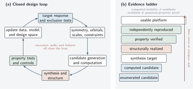
Materials design has two coupled directions. The loop updates models with measured successes and failures; the ladder prevents computational screening, synthesis, structural identification, property verification, and reproduction from being collapsed into one claim.

Stability Is a Hierarchy

Formation energy is only the first comparison

For a compound $M$ containing $x_a$ atoms of element $a$, a zero-temperature formation energy relative to chosen elemental reference states is

$$\Delta H_f(M) = E(M) - \sum_a x_a\mu_a^{\mathrm{elem}}.$$

A negative formation energy means that $M$ is favored over those elemental references within the calculation. It does not establish stability against decomposition into other compounds.

For a fixed overall composition $\mathbf x_M$, the convex-hull distance is

$$\begin{aligned} E_{\mathrm{hull}}(M) ={}& E(M)-E_{\mathrm{mix}}^{\min}, \\ E_{\mathrm{mix}}^{\min} ={}& \min_{\{\lambda_j\}} \sum_j\lambda_j E_j, \end{aligned}$$

subject to

$$\begin{aligned} \lambda_j&\ge0, & \sum_j\lambda_j&=1, \\ \sum_j\lambda_j\mathbf x_j &= \mathbf x_M. \end{aligned}$$

$E_{\mathrm{hull}}=0$ means stable against the included competing phases at the stated computational level. A small positive value means metastable by that comparison, not impossible to synthesize. The hull can change when a missing polymorph is found, magnetic order is altered, numerical settings change, or a more accurate energy model is used.

Temperature, pressure, and reservoirs matter

At finite temperature and in open chemical environments, a relevant potential may contain

$$\begin{aligned} \Phi ={}& E_{\mathrm{el}} +F_{\mathrm{vib}}(T) +F_{\mathrm{el}}(T) +pV \\ & -TS_{\mathrm{conf}} -\sum_a \mu_aN_a. \end{aligned}$$

Vibrational and configurational entropy can reorder close polymorphs. Gas partial pressures and chemical potentials matter for oxides, hydrides, chalcogenides, and growth under flux. Surfaces and interfaces alter the balance in thin films and nanoparticles. A zero-kelvin bulk hull is therefore one layer of evidence, not the whole synthesis problem.

Stability does not imply synthesizability

Four further questions are distinct:

• Dynamical stability: are phonon frequencies real over the relevant Brillouin zone, within converged numerical accuracy?
• Mechanical stability: does the elastic tensor satisfy the appropriate stability conditions?
• Kinetic accessibility: can available precursors reach the phase before becoming trapped in intermediates or losing volatile components?
• Persistence: does the product survive cooling, air exposure, cycling, and measurement?

Conversely, many useful materials are metastable. Epitaxy, pressure quenching, topotactic reactions, rapid cooling, ion exchange, and nanoscale confinement can select states above the bulk equilibrium hull. The correct design question is not “is $E_{\mathrm{hull}}$ below one universal cutoff?” It is “what thermodynamic and kinetic evidence supports this synthesis route for this material class?”

Symmetry and Topology as Design Principles

Work backward from the protected response

Symmetry can turn an unconstrained search into a structured one. A design ledger should identify:

1. the relevant space or magnetic space group;
2. Wyckoff positions and site symmetries;
3. active orbital characters and electron filling;
4. spin–orbit, exchange, crystal-field, and hybridization scales;
5. the symmetry preserved by the bulk, surface, substrate, strain, and magnetic state;
6. the observable expected from the proposed topology.

For an isolated group of weakly interacting bands, let $\mathbf n$ collect the multiplicities of irreducible representations at high-symmetry momenta. Compatibility requires

$$\mathcal C\mathbf n = \mathbf0.$$

Atomic band representations generate vectors $\mathbf b_\alpha$. If

$$\mathbf n = \sum_\alpha q_\alpha\mathbf b_\alpha, \qquad q_\alpha\in\mathbb Z_{\ge0},$$

then the symmetry data are compatible with an atomic limit under the stated assumptions. Failure of such a nonnegative decomposition can diagnose an obstruction. Symmetry indicators package related quotient information and enable large-scale screening.

Symmetry of Bloch States owns the little-group irreducible-representation labels and compatibility relations assumed by this vector test. This page owns their use in materials screening, synthesis-aware design, uncertainty tracking, and evidence limits.

The inference has limits:

• a nonzero indicator can certify topology only within its symmetry, gap, filling, and band-theory assumptions;
• a zero indicator does not exclude topology invisible to that indicator;
• incompatible labels may describe a symmetry-enforced semimetal rather than an insulator;
• DFT can misorder bands, underestimate gaps, or choose the wrong magnetic state;
• strong interactions can invalidate a one-electron classification or replace it with a many-body problem.

A topological candidate is not yet a useful material

After a band diagnosis, one must still determine:

• whether a global gap exists and exceeds temperature, disorder, and measurement broadening;
• whether the chemical potential can be placed in the relevant gap;
• whether surface or edge states survive the actual termination and reconstruction;
• whether trivial accumulation layers, bulk carriers, or magnetic domains mimic the signal;
• whether contacts and fabrication preserve the protecting symmetry;
• whether transport, spectroscopy, and thermodynamics support one consistent mechanism.

Symmetry and topology are powerful filters because they state necessary structure. They do not remove chemistry, defects, or experimental identification from the problem.

Correlation and Dimensionality as Design Knobs

Use a scale vector, not a single ratio

A first pass through a correlated candidate can be organized by

$$\begin{aligned} \boldsymbol{\eta}_{\mathrm{el}} &= \left( \frac{U}{W}, \frac{J_{\mathrm H}}{W}, \frac{\lambda_{\mathrm{SO}}}{W}, \frac{t_\perp}{t_\parallel} \right), \\ \boldsymbol{\eta}_{\mathrm{env}} &= \left( \frac{k_{\mathrm B}T}{W}, \frac{\Gamma_{\mathrm{dis}}}{W}, \frac{\hbar\omega_{\mathrm{ph}}}{W} \right). \end{aligned}$$

$\boldsymbol{\eta}_{\mathrm{el}}$ collects electronic design ratios and $\boldsymbol{\eta}_{\mathrm{env}}$ collects operating and environmental ratios. $U$ and $J_{\mathrm H}$ summarize screened interactions in a stated active basis; $W$ is the relevant bandwidth; $\lambda_{\mathrm{SO}}$ measures spin–orbit coupling; $t_\perp/t_\parallel$ measures dimensional crossover; and $\Gamma_{\mathrm{dis}}$ and $\omega_{\mathrm{ph}}$ represent disorder and lattice scales. None is a universal material constant independent of orbital choice, screening environment, structure, and probe window.

Layered chemistry, epitaxial strain, pressure, gating, dielectric screening, moiré periodicity, and interfacial hybridization can move several entries of $\boldsymbol{\eta}$. This makes them genuine design knobs, but not independent ones. Reducing $W$ raises $U/W$, yet can also:

• increase sensitivity to inhomogeneity and localization;
• strengthen electron–phonon competition;
• reduce phase stiffness and coherence scales;
• make neglected longer-range interactions important;
• amplify uncertainty in small hopping parameters.

A narrow band is therefore an opportunity for competing orders, not a phase prescription. Flat Bands develops the additional roles of isolation and quantum geometry.

Dimensional reduction changes fluctuations and fabrication

Lower dimension can enhance interaction effects and increase electrostatic tunability. It can also strengthen thermal fluctuations, environmental screening changes, substrate coupling, edge effects, and sample-to-sample disorder. Low-Dimensional Quantum Matter owns the density-of-states and fluctuation analysis.

For design, dimensionality should be reported through measured or computed crossover scales: occupied subband spacing, interlayer hopping, coherence lengths, screening length, thickness dependence, and the temperature at which neighboring layers lock together. Calling a material “two-dimensional” from morphology alone is not enough.

Correlated calculations need wider uncertainty budgets

When $U/W$ or multiorbital competition is large, semilocal DFT screening may still generate structures and broad trends, but its property ranking can be unreliable. A stronger workflow records the active orbitals, magnetic initial states, interaction parameters, double counting, solver, and sensitivity to competing structures. Agreement with one fitted observable is not prospective validation. The model-to-material standards are developed in Hubbard Physics in Materials.

Computation-Guided Synthesis

Use fidelity in stages

Computational effort should increase only as candidates survive tests appropriate to the claim:

1. Validity: charge balance where meaningful, geometric sanity, duplicate removal, and basic chemical constraints.
2. Fast screening: relaxed energies and approximate properties with a consistent method.
3. Convergence: basis, $k$ mesh, supercell, magnetic initialization, force, and solver tolerances.
4. Higher fidelity: improved exchange–correlation treatment, spin–orbit coupling, phonons, defects, finite-temperature terms, or many-body methods where the target requires them.
5. Synthesis planning: competing phases, precursors, reaction pathways, chemical potentials, and likely failure modes.
6. Prospective selection: choose candidates before the decisive calculation or experiment, then retain the failures.

Cross-code agreement is evidence of numerical precision only when the physical approximation and inputs are aligned. It does not measure exchange–correlation error. Conversely, two methods that disagree may expose model uncertainty rather than software failure. Convergence Tests and Error Estimates provide the general numerical framework.

Synthesis is an inference problem

A synthesis recipe specifies more than a nominal temperature. It includes precursor identity and purity, atmosphere and partial pressure, mixing and milling, crucible, geometry, ramp and dwell times, quench or cooling schedule, substrate, thickness, and post-processing. Each can select a different reaction path.

The A-Lab demonstration reported 36 obtained targets among 57 attempted inorganic powders over 17 days; 17 targets were not obtained and four outcomes were inconclusive. Only about 30% of its 353 tested recipes produced their targets, and many successful samples contained notable byproducts. The result is important evidence that databases, learned synthesis heuristics, robotics, diffraction analysis, and active learning can form a closed loop. It is not evidence that arbitrary predicted crystals are automatically synthesizable.

Failed recipes are scientifically useful when their conditions and products are retained. They constrain kinetic pathways, reveal precursor volatility and amorphization, and reduce publication bias. A model trained only on successful literature procedures learns from a selected record in which many boundaries of the synthesis window are absent.

Data-Driven Materials Discovery

Keep labels and provenance attached

Computed and experimental data should not be merged under an unlabeled “ground truth” column. A band gap may mean a Kohn–Sham value, a quasiparticle calculation, an optical onset, an activation scale, or a fitted transport parameter. Crystal records may be measured structures, relaxed hypothetical structures, disordered averages, or generated candidates. Every datum needs:

• quantity definition and units;
• computational or experimental protocol;
• structure, composition, and sample identity;
• uncertainty or convergence information;
• provenance, license, version, and date;
• known transformations and exclusions.

Representations should respect the intended invariances, such as translation, rotation, permutation of equivalent atoms, and periodicity. An invariant architecture does not guarantee physical extrapolation; it only removes some avoidable representational inconsistency.

Test the discovery regime, not a random interpolation task

Random train–test splits can place near-duplicate compositions or structures on both sides of the split. That measures interpolation within a redundant database and can substantially overestimate performance for unfamiliar candidates.

Choose a split that matches the proposed use:

• temporal split: train on data available before a cutoff and test on later records;
• chemical-family split: hold out an element family, prototype, or composition region;
• structure split: separate distinct structural clusters or space groups;
• property-tail split: test candidates beyond the training range;
• laboratory split: test transfer across instruments, synthesis teams, or processing conventions;
• prospective test: freeze the model, nominate candidates, and evaluate new outcomes.

Report both in-distribution and out-of-distribution performance. A calibrated model should also state when a candidate lies outside its support.

Acquisition functions encode scientific priorities

In sequential learning, a surrogate gives a predictive distribution

$$p(y\mid x,\mathcal D),$$

and the next candidate is chosen by

$$x_{\mathrm{next}} = \operatorname*{arg\,max}_{x\in\mathcal X_{\mathrm{avail}}} a(x\mid\mathcal D).$$

The acquisition $a$ may favor expected improvement, uncertainty reduction, diversity, Pareto-front resolution, or information about a phase boundary. It should also include experimental cost, batch constraints, safety, and the possibility that no candidate is worth testing. Active learning is useful because it makes this decision rule explicit, not because the algorithm is automatically unbiased.

Uncertainty must survive the handoffs

A schematic uncertainty budget is

$$\begin{aligned} \sigma_{\mathrm{tot}}^2 \approx{}& \sigma_{\mathrm{num}}^2 +\sigma_{\mathrm{model}}^2 +\sigma_{\mathrm{data}}^2 \\ & +\sigma_{\mathrm{synth}}^2 +\sigma_{\mathrm{meas}}^2. \end{aligned}$$

This sum assumes independent, approximately variance-like terms. Real errors are often correlated: one structural bias can affect the computed energy, training labels, synthesis choice, and diffraction fit. A useful report names correlations and irreducible ambiguities rather than forcing every uncertainty into one Gaussian interval.

Generative models require a staged evaluation. Validity asks whether an output describes a legal composition and periodic structure. Uniqueness and novelty compare it with training and reference sets. Stability requires calculations against competing phases. Synthesizability requires a route and experimental evidence. Function requires the target measurement. Passing the first two does not imply the last three.

Caution About Hype and Reproducibility

Translate large numbers into claim levels

Large-scale screening can produce millions of structures. Merchant and collaborators reported 2.2 million candidates below a previous convex hull and 381,000 entries on an updated calculated hull in their 2023 workflow. The same paper notes that future competing structures can displace hull entries and that finite-temperature stability and synthesizability remain open. Those numbers measure the reach of candidate generation plus machine-learning-assisted DFT validation, not millions of experimentally isolated materials.

Use precise verbs:

Evidence	Defensible verb
generated structure passes syntax checks	enumerated
surrogate ranks a candidate	predicted by the stated model
converged calculation places it on a stated hull	computationally stable within that reference set
diffraction requires the target phase	structurally detected
quantitative refinement establishes a substantial phase fraction	synthesized with the reported purity
independent observables establish the response	property verified
independent production and measurement agree	reproduced

“Discovered” should be accompanied by the rung reached.

A reproducibility manifest

For a computational candidate, preserve:

• input and relaxed structures with stable identifiers;
• code, version, build, workflow, and random seeds;
• functional, basis or cutoff, pseudopotentials, $k$ mesh, smearing, and convergence thresholds;
• spin–orbit and magnetic settings, including all initial states tested;
• Hubbard parameters, orbital projectors, and double counting where used;
• competing phases, database snapshots, corrections, and hull construction;
• raw outputs, parsed data, exclusions, and uncertainty estimates.

For synthesis and measurement, add:

• precursor suppliers, lots, purities, storage, and handling;
• atmosphere, pressure, geometry, ramps, dwell times, and cooling;
• sample identifiers linking every processing step and measurement;
• calibration files, backgrounds, fitting code, and alternative fits;
• phase fractions, spatial variation, defects, null results, and failed batches;
• a frozen prospective protocol and an independent replication where the claim warrants it.

FAIR data are findable, accessible, interoperable, and reusable. FAIR does not mean error-free, and open files without semantic metadata may still be unusable. Reproducibility is likewise not identical to truth: precisely repeating a biased method reproduces the bias. Trust grows when numerical precision, model adequacy, synthesis repeatability, and independent physical observables are tested separately.

A Practical Design Workflow

1. Write the claim sentence first. Include the observable, operating window, sample form, and comparison baseline.
2. Derive necessary conditions. State which symmetry, filling, orbital, interaction, dimensional, and stability features are required and which are merely helpful.
3. Define the candidate universe. Record excluded elements, prototypes, processing limits, and database snapshot.
4. Choose a Pareto problem. Keep competing objectives visible and attach uncertainty to each coordinate.
5. Screen in tiers. Reserve expensive methods for candidates that survive cheaper falsification tests.
6. Plan synthesis before final ranking. Include precursors, competing phases, kinetics, and characterization access.
7. Freeze prospective predictions. Separate model development from the final candidate test.
8. Measure structure before mechanism. Quantify phase purity, stoichiometry, defects, and spatial variation.
9. Use orthogonal property probes. Require observables with different confounders.
10. Publish the loop. Release successes, nulls, failures, metadata, code, and the rule used to choose the next experiment.

Common Mistakes

• Treating negative formation energy as stability against every decomposition route.
• Applying one universal energy-above-hull cutoff across unrelated chemistries and synthesis methods.
• Calling a generated or relaxed structure a synthesized material.
• Equating a symmetry indicator with a measured topological response.
• Maximizing $U/W$ without tracking disorder, phonons, stiffness, and uncertainty in $W$.
• Reporting random-split accuracy for an out-of-distribution discovery claim.
• Combining computed and experimental labels without provenance.
• Omitting failed syntheses and thereby teaching the next model only a selected history.
• Fitting a property and citing that same property as validation.
• Reporting only the best magnetic initialization, polymorph, sample, or model seed.
• Treating automation as autonomy without a documented decision rule and stopping condition.
• Using “AI discovered” without identifying which evidence rung was actually reached.

Exercises

1. Convex-hull distance

At composition $A_{1/2}B_{1/2}$, a candidate has energy $-0.62\,\mathrm{eV/atom}$. A mixture of two neighboring stable phases at the same overall composition has energy $-0.67\,\mathrm{eV/atom}$. Compute $E_{\mathrm{hull}}$. What does the result establish?

Solution

The hull distance is

$$\begin{aligned} E_{\mathrm{hull}} &= -0.62 -(-0.67) \\ &= 0.05\,\mathrm{eV/atom} = 50\,\mathrm{meV/atom}. \end{aligned}$$

Within this zero-temperature energy model and included phase set, the candidate is metastable by $50\,\mathrm{meV/atom}$. The number does not prove that synthesis will fail. A claim about accessibility also needs uncertainty in relative energies, missing competitors, finite-temperature terms, and a material-class-specific kinetic or synthesis argument.

2. Pareto dominance

Three candidates have coordinates $(P,S,C)$, where property $P$ and synthesis score $S$ are maximized and cost $C$ is minimized:

Candidate	$P$	$S$	$C$
A	8	5	4
B	7	6	3
C	6	4	5

Which candidates are Pareto-optimal?

Solution

A and B trade property against synthesis score and cost: A has larger $P$, while B has larger $S$ and lower $C$. Neither dominates the other.

B dominates C because $7>6$, $6>4$, and $3<5$. A also dominates C because $8>6$, $5>4$, and $4<5$. The Pareto set is therefore $\{\mathrm A,\mathrm B\}$. Choosing one requires a stated preference or constraint; the data alone do not define a unique winner.

3. Interpret a zero symmetry indicator

A nonmagnetic calculation with spin–orbit coupling gives a zero symmetry indicator for an isolated occupied-band set. A report concludes that the material is topologically trivial. Diagnose the inference and name three next checks.

Solution

The conclusion is too strong. A zero indicator means that this indicator does not diagnose a nontrivial class under the assumed symmetry and band ordering. Some topological phases are invisible to symmetry indicators.

Useful next checks are:

1. compute the relevant Wilson loops, Berry phases, or direct invariants;
2. verify a global gap and repeat the band ordering with a justified higher-fidelity method;
3. test the actual magnetic structure, filling, and structural symmetry.

If a surface response is claimed, termination-resolved surface calculations and experimental exclusion of trivial surface bands are additional requirements.

4. Narrowing a correlated band

Strain reduces a target bandwidth from $W=0.40\,\mathrm{eV}$ to $0.20\,\mathrm{eV}$ while a screened interaction estimate remains $U=0.80\,\mathrm{eV}$. Disorder broadening rises from $20$ to $60\,\mathrm{meV}$. Compare $U/W$ and $\Gamma_{\mathrm{dis}}/W$ before and after strain.

Solution

Initially,

$$\frac{U}{W}=2, \qquad \frac{\Gamma_{\mathrm{dis}}}{W} = \frac{0.020}{0.40} = 0.05.$$

After strain,

$$\frac{U}{W}=4, \qquad \frac{\Gamma_{\mathrm{dis}}}{W} = \frac{0.060}{0.20} = 0.30.$$

The interaction ratio doubles, but the relative disorder scale increases by a factor of six. The design has moved toward stronger nominal correlation and toward much stronger inhomogeneous broadening or localization. A claim that strain simply “enhances correlation” omits a competing change that may dominate the measured state.

5. Design a leakage-resistant validation split

A database contains many substitutions within the same structural prototypes. The intended model will propose compounds in prototypes absent from today’s literature. Why is a random split inadequate, and what split should be used?

Solution

A random split is likely to place nearly identical structures or substitution families in both training and test sets. Strong performance can then reflect interpolation among redundant neighbors rather than transfer to new prototypes.

Cluster structures using a representation chosen before examining the test labels, assign entire structural clusters or prototypes to the held-out set, and report the similarity of every test item to training data. A temporal split can be layered on top: train on a frozen historical snapshot and test on later structures from held-out families. The final evidence should be prospective, with the model frozen before new calculations or syntheses are performed.

6. Audit an AI-discovery claim

A press release says that an AI “discovered two million stable materials.” The associated work generated structures, ranked them with a graph model, and relaxed selected candidates using DFT against a database hull. No new synthesis was reported. Rewrite the claim and list four missing steps before calling one candidate a property-verified material.

Solution

A defensible statement is: “The workflow generated and screened roughly two million crystal candidates predicted to be stable relative to the stated calculated reference set; a smaller subset remained on the updated computational convex hull.” Exact numbers and filtering definitions should follow the paper.

Before a candidate becomes property verified, at least four further steps are:

1. test numerical, functional, magnetic, vibrational, defect, and competing-phase uncertainty;
2. identify and execute a plausible synthesis route;
3. establish composition, structure, phase fraction, and defects experimentally;
4. measure the target quantum property with controls that reject competing mechanisms.

Independent synthesis and measurement would move the claim to the next rung, reproduced material.

Research Status

• Established: high-throughput electronic-structure databases; symmetry-guided band screening; convex-hull analysis at a stated approximation; convergence benchmarks; Bayesian and other sequential-learning workflows; automated synthesis and characterization in bounded domains.
• Active: reliable finite-temperature stability; reaction-path prediction; calibrated uncertainty outside known chemical families; strongly correlated materials screening; integration of computation, robotics, and human constraints; transferable synthesis models; prospective multi-laboratory benchmarks.
• Conjectural: that current foundation or generative models can extrapolate broadly enough to transform arbitrary generated crystals into experimentally useful quantum materials without domain-specific retraining and extensive physical filtering.
• Speculative: fully autonomous, general-purpose discovery systems that choose scientifically important questions, invent unrestricted synthesis routes, establish mechanisms, and validate devices without substantial human judgment.

These categories can change with the domain. Autonomous phase mapping in a fixed composition spread and autonomous discovery across unrestricted chemistry are not the same technical claim.

Use Quantum Matter Frontiers and Open Problems when a ranked candidate needs a dated audit of held-out validation, domain shift, synthesis, property verification, independent reproduction, falsifiers, and the boundary between a material result and a technology claim.

Connections

• How Quantum Matter Is Measured turns a target observable into an auditable measurement contract and separates raw records, calibrated quantities, inferred material properties, and phase claims.
• Device Fabrication Concepts tests whether a candidate survives contacts, gates, patterning, assembly, encapsulation, cryogenic integration, and independent device batches.
• Quantum Matter Map supplies the structure, scale, response, and evidence ledgers used to formulate a target.
• Topology in Quantum Matter develops invariants, bulk–boundary correspondence, and experimental topology claims.
• Symmetry-Protected Topological Phases gives the many-body definition of symmetry protection.
• Hubbard Physics in Materials owns active subspaces, screened interactions, correlated solvers, and model discrimination.
• Low-Dimensional Quantum Matter explains dimensional crossover, density of states, fluctuations, and experimental diagnostics.
• Engineered Heterostructures treats interface transfer, compatibility, and proximity-phase evidence.
• Artificial Lattices and Designer Matter compares programmable graph realizations with natural-material discovery.
• Flat Bands develops bandwidth, isolation, projector geometry, and correlated flat-band criteria.
• Convergence Tests and Error Estimates provide the general numerical evidence standards.

Further Reading

• A. Jain et al., “The Materials Project: A Materials Genome Approach to Accelerating Materials Innovation,” for the architecture and purpose of an open high-throughput database.
• D. N. Basov, R. D. Averitt, and D. Hsieh, “Towards Properties on Demand in Quantum Materials,” for a physics-centered view of controlling collective states.
• B. Bradlyn et al., “Topological Quantum Chemistry,” together with H. C. Po, A. Vishwanath, and H. Watanabe on symmetry indicators, for symmetry-led band diagnosis and its scope.
• M. Scheffler et al., “FAIR Data Enabling New Horizons for Materials Research,” for data provenance and stewardship.
• A. Merchant et al. and N. Szymanski et al., read together, for the distinction between large-scale computational stability screening and automated experimental synthesis.

References

1. A. Jain et al., “Commentary: The Materials Project: A Materials Genome Approach to Accelerating Materials Innovation,” APL Materials 1, 011002 (2013), doi:10.1063/1.4812323.
2. S. Curtarolo et al., “AFLOWLIB.ORG: A Distributed Materials Properties Repository from High-Throughput ab Initio Calculations,” Computational Materials Science 58, 227–235 (2012), doi:10.1016/j.commatsci.2012.02.002.
3. J. E. Saal, S. Kirklin, M. Aykol, B. Meredig, and C. Wolverton, “Materials Design and Discovery with High-Throughput Density Functional Theory: The Open Quantum Materials Database,” JOM 65, 1501–1509 (2013), doi:10.1007/s11837-013-0755-4.
4. W. Sun et al., “The Thermodynamic Scale of Inorganic Crystalline Metastability,” Science Advances 2, e1600225 (2016), doi:10.1126/sciadv.1600225.
5. K. Lejaeghere et al., “Reproducibility in Density Functional Theory Calculations of Solids,” Science 351, aad3000 (2016), doi:10.1126/science.aad3000.
6. N. Mounet et al., “Two-Dimensional Materials from High-Throughput Computational Exfoliation of Experimentally Known Compounds,” Nature Nanotechnology 13, 246–252 (2018), doi:10.1038/s41565-017-0035-5.
7. B. Bradlyn et al., “Topological Quantum Chemistry,” Nature 547, 298–305 (2017), doi:10.1038/nature23268.
8. H. C. Po, A. Vishwanath, and H. Watanabe, “Symmetry-Based Indicators of Band Topology in the 230 Space Groups,” Nature Communications 8, 50 (2017), doi:10.1038/s41467-017-00133-2.
9. T. Zhang et al., “Catalogue of Topological Electronic Materials,” Nature 566, 475–479 (2019), doi:10.1038/s41586-019-0944-6.
10. D. N. Basov, R. D. Averitt, and D. Hsieh, “Towards Properties on Demand in Quantum Materials,” Nature Materials 16, 1077–1088 (2017), doi:10.1038/nmat5017.
11. H. Y. Hwang et al., “Emergent Phenomena at Oxide Interfaces,” Nature Materials 11, 103–113 (2012), doi:10.1038/nmat3223.
12. D. M. Kennes et al., “Moiré Heterostructures as a Condensed-Matter Quantum Simulator,” Nature Physics 17, 155–163 (2021), doi:10.1038/s41567-020-01154-3.
13. K. T. Butler, D. W. Davies, H. Cartwright, O. Isayev, and A. Walsh, “Machine Learning for Molecular and Materials Science,” Nature 559, 547–555 (2018), doi:10.1038/s41586-018-0337-2.
14. P. Raccuglia et al., “Machine-Learning-Assisted Materials Discovery Using Failed Experiments,” Nature 533, 73–76 (2016), doi:10.1038/nature17439.
15. A. G. Kusne et al., “On-the-Fly Closed-Loop Materials Discovery via Bayesian Active Learning,” Nature Communications 11, 5966 (2020), doi:10.1038/s41467-020-19597-w.
16. K. M. Jablonka et al., “Bias Free Multiobjective Active Learning for Materials Design and Discovery,” Nature Communications 12, 2312 (2021), doi:10.1038/s41467-021-22437-0.
17. N. Szymanski et al., “An Autonomous Laboratory for the Accelerated Synthesis of Novel Materials,” Nature 624, 86–91 (2023), doi:10.1038/s41586-023-06734-w.
18. A. Merchant et al., “Scaling Deep Learning for Materials Discovery,” Nature 624, 80–85 (2023), doi:10.1038/s41586-023-06735-9.
19. S. S. Omee et al., “Structure-Based Out-of-Distribution Materials Property Prediction: A Benchmark Study,” npj Computational Materials 10, 144 (2024), doi:10.1038/s41524-024-01316-4.
20. K. Li et al., “Exploiting Redundancy in Large Materials Datasets for Efficient Machine Learning with Less Data,” Nature Communications 14, 7283 (2023), doi:10.1038/s41467-023-42992-y.
21. M. D. Wilkinson et al., “The FAIR Guiding Principles for Scientific Data Management and Stewardship,” Scientific Data 3, 160018 (2016), doi:10.1038/sdata.2016.18.
22. M. Scheffler et al., “FAIR Data Enabling New Horizons for Materials Research,” Nature 604, 635–642 (2022), doi:10.1038/s41586-022-04501-x.

Summary

Quantum-materials design is a closed, multiobjective inference problem. Symmetry, topology, correlation, and dimensionality can narrow the search, but each comes with assumptions and competing scales. Formation energies and calculated convex hulls rank candidates within a model; synthesis adds kinetics, precursors, finite temperature, defects, and persistence. Data-driven methods are most credible when tested on the out-of-distribution regime they claim to serve and when uncertainty, failed experiments, and decision rules remain visible. A material advances from enumeration to computation, synthesis, property verification, reproduction, and use only by adding distinct evidence at every rung.