Graphene

Graphene is a single sheet of $sp^2$-bonded carbon whose low-energy $\pi$ bands form two time-reversed Dirac valleys. In an engineered-materials setting, however, the central question is not merely why an ideal cone appears. It is which physical operation adds which low-energy operator, which symmetry that operator preserves, and which observation can distinguish it from disorder, contacts, strain, or many-body renormalization.

That operator-first view keeps several statements separate:

1. a honeycomb lattice does not by itself guarantee a gapless cone;
2. a shifted or distorted cone is not necessarily gapped;
3. graphene’s unconventional integer quantum Hall sequence is not automatically a zero-field anomalous Hall phase;
4. strain can act as a valley-odd gauge field without breaking time reversal;
5. a moiré pattern creates a new translation group, but not automatically a flat or correlated band.

Canonical Scope

This page is the canonical home for graphene as an engineered materials platform. It owns the perturbation ledger, Hall nomenclature, strain-induced scalar and pseudogauge fields, the distinction between real and pseudomagnetic response, substrate and interface controls, and the handoff from monolayer Dirac kinematics to moiré coupling.

Graphene and Dirac Materials owns the full honeycomb tight-binding construction, Dirac-cone expansion, pseudospin winding, Berry phase, Landau-level derivation, and monolayer transport diagnostics. Tight-Binding Models owns the general localized-orbital method. Integer Quantum Hall Effect owns plateau formation, localization, edge channels, and metrology. Two-Dimensional Materials owns the generic environmental-screening, heterostructure, exciton, and gate-control ledgers.

The compact equations below are therefore interface contracts, not duplicate derivations. They identify what an engineering perturbation means in the already-established low-energy basis.

Honeycomb and Dirac Baseline

Fix the basis before naming a perturbation

Let $\tau=\pm1$ label the two valleys, let $\mathbf p=-i\hbar\nabla$ measure momentum from the appropriate valley center, and let $\sigma_i$ act on the $A/B$ sublattice spinor. One convenient convention is

$$\boldsymbol{\sigma}_\tau \equiv (\tau\sigma_x,\sigma_y), \qquad H_\tau^{(0)} = v_F\boldsymbol{\sigma}_\tau\cdot\mathbf p.$$

Changing valley, unit-cell, Bloch-phase, or sublattice conventions can move signs among $\tau$, $\sigma_x$, and $\sigma_y$. Physical spectra and gauge-invariant response do not depend on that bookkeeping, but a quoted mass sign or pseudogauge field does. Every effective Hamiltonian should therefore state its spinor and valley convention.

Write $V_\Sigma(\mathbf r)\equiv V_{\mathrm{ext}}(\mathbf r)+V_s(\mathbf r)$ and define $\Pi_{\tau,j}\equiv p_j+eA_j+\tau eA_{s,j}$. A useful engineering expansion is

$$\begin{aligned} H_\tau ={}& V_\Sigma\mathbb I + v_{ij}\sigma_{\tau,i}\Pi_{\tau,j} \\ &+ \left( \Delta_S+\tau\Delta_H \right)\sigma_z \\ &+ H_{\mathrm{so}}+H_{\mathrm{iv}}+\cdots . \end{aligned}$$

Here $e>0$, so $\mathbf p+e\mathbf A$ is the electromagnetic minimal coupling for an electron. The strain field $\mathbf A_s$ is written in the same units as a vector potential. The velocity tensor $v_{ij}$ allows anisotropy and spatial variation. $H_{\mathrm{iv}}$ mixes valleys and cannot be represented inside one fixed-$\tau$ block.

Low-energy term	Representative source	Leading consequence
$V\mathbb I$	gate potential, charged disorder, deformation potential	shifts local energy without opening a sublattice gap
$\Delta_S\sigma_z$	sublattice inequivalence, aligned substrate	opens a time-reversal-symmetric Dirac mass
$\tau\Delta_H\sigma_z$	time-reversal-breaking complex hopping or an effective Chern mass	can make the two valleys add to a Chern response
$e\mathbf A$	real magnetic field	couples with the same charge sign in both valleys
$\tau e\mathbf A_s$	smooth nonuniform bond strain	couples with opposite signs in time-reversed valleys
$H_{\mathrm{iv}}$	atomic defects, armchair edges, short-period potentials	invalidates an independently conserved valley label
$H_{\mathrm{so}}$	intrinsic, Rashba, or proximity spin–orbit coupling	entangles real spin with sublattice, valley, or momentum

This table is a low-energy classification, not a unique microscopic inversion. Several sources can generate the same symmetry-allowed operator, and a real interface generally produces several terms at once.

Pseudospin is an operator ledger

For an ideal band with sign $s=\pm1$,

$$\left\langle \boldsymbol{\sigma}_\tau \right\rangle = s\,\widehat{\mathbf p}.$$

The expectation value records sublattice phase coherence. A scalar potential tests spinor overlap differently from a sublattice mass or intervalley defect; this is why the ideal suppression of exact intravalley backscattering does not imply immunity to resistance.

In a device, the useful question is therefore not “is pseudospin present?” Every two-component low-energy state has some spinor structure. The useful questions are:

• which microscopic orbitals define the two components;
• which symmetry constrains their relative phase;
• which perturbation operator the probe applies;
• whether valley mixing or a mass tilts the pseudospin away from the ideal plane;
• over what energy and length window the two-band projection remains controlled.

The complete winding and overlap derivations remain at Graphene and Dirac Materials.

Hall Physics Without a Naming Trap

The unconventional integer sequence uses a real field

For a perpendicular real magnetic field, the ideal monolayer Dirac levels are

$$E_n = \operatorname{sgn}(n) v_F \sqrt{2e\hbar|B|\,|n|}, \qquad n\in\mathbb Z,$$

with a zero-energy level and approximate fourfold spin–valley degeneracy before Zeeman, interaction, substrate, or lattice-scale splittings are resolved. The corresponding ideal filling sequence is

$$\nu = 4\left(N+\frac12\right) = \pm2,\pm6,\pm10,\ldots,$$

and $\sigma_{xy}=\nu e^2/h$. The offset is historically called an anomalous or half-integer quantum Hall effect, but the measured total Hall conductance is still an integer multiple of $e^2/h$. Plateau formation still requires localization and edge transport; the single-particle ladder alone is insufficient.

A zero-field anomalous Hall phase is a different claim

The modern phrase quantum anomalous Hall effect usually means a quantized Hall response at zero applied magnetic field, supported by a nonzero Chern number and broken time reversal. For two massive Dirac valleys, the magnitude of the filled-band Chern number has the schematic form

$$|C| = \frac12 \left| \operatorname{sgn}m_K - \operatorname{sgn}m_{K'} \right|.$$

The overall sign depends on orientation and Hamiltonian conventions. Equal-sign sublattice masses give cancelling valley contributions and $C=0$; opposite-sign masses can give $|C|=1$. Thus a gap at charge neutrality is not enough. A zero-field Chern claim needs broken-time-reversal evidence, a bulk mobility gap, chiral edge response, reproducible Hall quantization, and controls against ordinary magnetic hysteresis or parallel conduction.

This distinction resolves an ambiguity in the older phrase “anomalous quantum Hall effect in graphene”: it may refer to the unconventional real-field sequence rather than a zero-field Chern phase.

Strain and Pseudogauge Fields

Bond deformation enters through geometry and hopping

Let $\mathbf u(\mathbf r)$ be the in-plane displacement and $h(\mathbf r)$ the out-of-plane height. To leading nonlinear order, the membrane strain tensor is

$$u_{ij} = \frac12 \left( \partial_i u_j + \partial_j u_i + \partial_i h\,\partial_j h \right).$$

If the three nearest-neighbor bonds change by $\delta\ell_n$, a common linearized hopping model is

$$t_n \simeq t_0 \left( 1-\beta\frac{\delta\ell_n}{a_{\mathrm{cc}}} \right),$$

where $a_{\mathrm{cc}}$ is the carbon–carbon distance and $\beta=-\partial\ln t/\partial\ln a_{\mathrm{cc}}$ is a dimensionless hopping-strain parameter. Its fitted value depends on the microscopic model and strain range.

For an axis convention with $x$ along a chosen zigzag direction, the leading valley-odd vector potential may be written

$$\begin{aligned} A_{s,x} &= \frac{\hbar\beta} {2ea_{\mathrm{cc}}} \left( u_{xx}-u_{yy} \right), \\ A_{s,y} &= -\frac{\hbar\beta} {ea_{\mathrm{cc}}} u_{xy}. \end{aligned}$$

Rotating the crystal axes rotates the tensor combination, and changing the valley or Bloch convention can reverse signs. Some authors define a wave-vector field $\boldsymbol{\mathcal A}_s=e\mathbf A_s/\hbar$ or use the graphene lattice constant instead of $a_{\mathrm{cc}}$; numerical comparisons must reconcile those conventions first.

Strain also generates a scalar deformation potential,

$$V_s \simeq g_D \left( u_{xx}+u_{yy} \right),$$

and generally changes $v_{ij}$. In inhomogeneous or curved sheets, geometric connection terms and higher gradients can matter. The pseudogauge-only Hamiltonian is a leading approximation, not the complete continuum theory.

Uniform strain shifts a cone; gradients create pseudoflux

Define

$$B_s = \partial_xA_{s,y} - \partial_yA_{s,x}.$$

A spatially uniform strain tensor gives a constant $\mathbf A_s$ and therefore $B_s=0$ in the bulk. It can move the valley centers and make velocities anisotropic, but a cone shift is not a pseudo-Landau quantization. Nonuniform strain, curvature-induced bond modulation, or boundary relaxation is required for nonzero pseudoflux.

Because the Hamiltonian contains $\tau e\mathbf A_s$, the effective field is opposite in the two valleys:

$$B_{\mathrm{eff},\tau} = \tau B_s.$$

Time reversal exchanges the valleys and reverses the effective field, so the complete strained system can preserve time reversal even though each valley separately resembles a charged Dirac particle in a magnetic field. Equal valley populations therefore do not acquire the net charge Hall response produced by a real field.

Pseudo-Landau levels are local, valley paired, and conditional

If $B_s$ varies slowly on the magnetic length

$$\ell_{B_s} = \sqrt{\frac{\hbar}{e|B_s|}},$$

the local spectrum can approximate

$$E_{n,\tau}-V_s \simeq \operatorname{sgn}(n) v_F \sqrt{ 2e\hbar|B_s|\,|n| }.$$

The level energies depend on $|B_s|$, while their valley and sublattice wave functions remember the sign reversal. In the simplest convention, the pseudo-$n=0$ states from the two valleys can occupy the same physical sublattice, unlike the opposite-sublattice pattern for a uniform real field.

A controlled local-Landau description needs a scale window such as

$$a_{\mathrm{cc}} \ll \ell_{B_s} \ll L_{\mathrm{strain}},$$

where $L_{\mathrm{strain}}$ is the variation scale of the effective field. Atomic reconstruction invalidates the smooth-valley expansion at the lower end; rapid field variation destroys a local Landau ladder at the upper end.

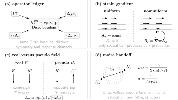
An operator and scale ledger for engineered graphene. Scalar, sublattice-mass, Chern-mass, and strain terms modify the same Dirac baseline in different symmetry channels. Uniform strain gives a constant valley-odd vector potential but no bulk pseudofield; a strain gradient produces opposite effective fields in $K$ and $K'$. Twisting two Dirac layers introduces the momentum mismatch $k_\theta$, moiré period $L_M$, and coupling ratio $\alpha=w/(\hbar v_Fk_\theta)$.

Evidence for a pseudomagnetic field

Scanning tunnelling spectroscopy on graphene nanobubbles has reported peaks consistent with a Dirac $\sqrt{|n|}$ pseudo-Landau sequence and very large local effective fields. The quoted field is inferred from a local spectral model; it is not a statement that a uniform hundreds-of-tesla electromagnetic flux threads the whole device.

A persuasive strain-field assignment combines:

1. atomic topography or diffraction sufficient to reconstruct strain;
2. a continuum or atomistic conversion from bonds to $\mathbf A_s$ with conventions stated;
3. local spectral peaks following the Dirac Landau index dependence;
4. spatial evolution consistent with the inferred $B_s(\mathbf r)$;
5. valley and sublattice behavior compatible with a time-reversal-preserving pseudofield;
6. controls against confinement resonances, tip-induced potentials, real magnetic flux, moiré minibands, and ordinary disorder.

Raman shifts, polarization, and linewidths can map strain and doping but do not alone establish pseudoflux. Likewise, a fitted $\sqrt{|n|}$ sequence without an independently constrained strain field is suggestive rather than complete.

Substrates, Encapsulation, and Proximity

There is no substrate-free device Hamiltonian

Suspended graphene approaches a mechanically isolated sheet but still has strain, adsorbates, contacts, gates, and edge boundary conditions. Encapsulated graphene trades exposed-surface disorder for a designed dielectric and crystallographic environment. Neither geometry is simply “pristine.”

Engineering element	Possible low-energy terms	Required control
misaligned hBN encapsulation	smoother scalar disorder, dielectric screening, residual strain	mobility, compressibility, Raman, spatial disorder map
aligned graphene–hBN	periodic scalar and sublattice potentials, relaxation, moiré minibands	alignment angle, satellite features, local registry, gap probe
metallic gate	carrier density, image-charge screening, displacement field	quantum capacitance, leakage, gate distance
magnetic substrate	exchange, magnetic disorder, possible Chern mass	magnetometry, hysteresis controls, edge and bulk transport
strong-spin–orbit neighbor	Rashba or valley-dependent spin–orbit terms	spin texture, weak antilocalization, spectroscopy
metal contact	doping, strain, intervalley scattering, mode mismatch	four-terminal geometry, contact resistance, local potential

Hexagonal boron nitride often improves charge homogeneity and mobility, but near crystallographic alignment it also creates a long-period potential and can relax into commensurate domains separated by strained walls. The same material can therefore be a clean dielectric, a symmetry-breaking substrate, and a moiré partner, depending on angle, pressure, cleanliness, and relaxation.

A measured gap needs an operator diagnosis

A neutrality-region suppression can arise from a sublattice mass, interaction order, finite-size confinement, localization, contact barriers, or inhomogeneous puddles. Transport activation measures a mobility or charge gap only under stated assumptions; scanning tunnelling measures a local spectral gap; capacitance measures compressibility; optical response probes neutral transitions.

The most direct route from a claimed gap to an engineered Hamiltonian is:

1. establish the atomic registry and layer environment;
2. identify which symmetry is broken;
3. measure both occupied and unoccupied spectral weight when possible;
4. compare bulk and edge transport;
5. reverse alignment, displacement field, magnetization, or strain;
6. show that the inferred term predicts held-out observables.

Graphene as a Foundation for Moiré Matter

Twist introduces a new momentum and length scale

For two graphene layers with relative angle $\theta$, let

$$K = \frac{4\pi}{3a}, \qquad k_\theta = 2K\sin\frac{\theta}{2},$$

where $a$ is the graphene lattice constant. Moiré Superlattices derives the ideal period $L_M$, the cell area $A_M$, and their mismatch and heterostrain corrections. For graphene’s fourfold spin–valley manifold, the density interval corresponding to four carriers per cell is

$$n_s = \frac{4}{A_M}.$$

These are geometric calibrations. Lattice relaxation, heterostrain, spatial twist disorder, and unequal lattice constants modify the local pattern and can broaden any density inferred from a single nominal angle.

Interlayer tunnelling competes with Dirac kinetic energy

A compact coupling ratio is

$$\alpha = \frac{w} {\hbar v_Fk_\theta},$$

where $w$ is an appropriate interlayer tunnelling scale. Small twist reduces $\hbar v_Fk_\theta$ and makes interlayer hybridization nonperturbative. This is the kinematic origin of strong velocity renormalization and narrow moiré bands in continuum descriptions.

The number $\alpha$ is not by itself a universal magic-angle criterion. Relaxation distinguishes local stacking regions and modifies tunnelling harmonics; heterostrain breaks rotational symmetry; remote hoppings and particle–hole asymmetry reshape bands; screening and gates change interactions; and disorder sets whether a narrow band is experimentally coherent.

Inherited from monolayer graphene	New in a moiré problem
two valleys and real spin	moiré translations and miniband indices
sublattice spinor and Dirac kinetic energy	layer spinor and interlayer tunnelling matrices
smooth-potential suppression of intervalley scattering	local stacking registry and lattice relaxation
Berry phase and valley-contrasting geometry	miniband Berry curvature and possible Chern bands
velocity, strain, dielectric, and disorder scales	twist angle, $L_M$, $w$, remote-band gaps, filling per moiré cell

Graphene supplies the degrees of freedom, but moiré translation changes the Hilbert-space organization. Twisted Bilayer Graphene develops the corresponding continuum model and the evidence for magic-angle flat bands, correlated states, superconductivity, and valley topology. None of those phases follows from observing a moiré wavelength or a narrow single-particle band alone.

Experimental Claim Ladder

Establish the platform before the phase

A reproducible workflow is:

1. Structure: determine layer number, stacking, twist, strain, bubbles, edges, and crystallographic axes.
2. Electrostatics: calibrate density, quantum capacitance, displacement field, leakage, contact doping, and dielectric thickness.
3. Single-particle structure: locate neutrality points, gaps, satellite bands, velocities, and degeneracies with more than one probe where possible.
4. Scattering: separate intervalley, intravalley, transport, quantum, and phase-coherence scales.
5. Symmetry: reverse field, valley selection, substrate magnetization, strain orientation, or layer alignment.
6. Collective evidence: only then infer interaction-driven order from gaps, hysteresis, thermodynamics, edge response, or phase coherence.

Match each claim to a measurement

Claim	Primary evidence	Important exclusion
Dirac dispersion	momentum-resolved band or Landau-level scaling	a merely linear transport curve
sublattice mass	local or momentum-resolved gap plus registry and symmetry	contact or localization gap
pseudomagnetic field	strain reconstruction plus valley-paired local Landau sequence	confinement or real flux
zero-field Chern phase	quantized Hall response, bulk gap, chiral edge, broken time reversal	ordinary anomalous Hall hysteresis
moiré miniband	structural period plus satellite spectrum and filling closure	topographic corrugation alone
correlated moiré phase	reproducible many-body gap or coherence with symmetry and control tests	narrow band or integer filling alone

Common Mistakes

• Repeating the ideal honeycomb derivation as if it diagnosed a device. The derivation establishes a baseline; the experiment still needs a perturbation and disorder ledger.
• Calling every neutrality suppression a Dirac mass. Spectral, mobility, contact, and interaction gaps are different observables.
• Using “anomalous quantum Hall” without stating whether a real field is present. The half-offset integer sequence and a zero-field Chern phase are distinct.
• Treating constant strain as a pseudomagnetic field. Only the curl of the pseudovector potential produces bulk pseudoflux.
• Forgetting the scalar deformation potential and velocity tensor. Strain does more than add $\mathbf A_s$.
• Assigning a net Hall effect to a time-reversal-symmetric pseudofield. Opposite valleys feel opposite effective fields and cancel in charge response when equally occupied.
• Quoting a pseudofield without its spatial scale. A large local fitted field is not a uniform macroscopic magnetic flux.
• Calling hBN an inert substrate. Alignment, relaxation, dielectric screening, and sublattice asymmetry can all matter.
• Inferring a magic angle from geometry alone. Tunnelling, relaxation, heterostrain, screening, and disorder set the actual band structure.
• Calling every moiré integer insulator a Mott state. Flavor order, topology, band gaps, charge order, and localization are competing explanations.

Exercises

Exercise 1: classify four perturbations

Consider $V_0\mathbb I$, $\Delta_S\sigma_z$, $\tau\Delta_H\sigma_z$, and a smooth constant $\mathbf A_s$. Which terms open a Dirac gap, which can support a zero-field Chern phase, and which merely shift energy or momentum?

Solution

$V_0\mathbb I$ shifts both bands and does not gap the cone. A constant $\mathbf A_s$ shifts the two valley centers in opposite directions and has zero bulk curl, so it also does not gap or Landau-quantize the ideal cone.

Both mass terms anticommute with the kinetic $\sigma_x$ and $\sigma_y$ matrices and open a gap. The sublattice mass has equal signs in the two valley blocks; opposite valley chiralities then cancel, giving total $C=0$ when time reversal is preserved. The Haldane-type mass changes sign between valleys, allowing the two half-integer valley contributions to add to $|C|=1$.

The operator classification does not prove that a microscopic device realizes any one term. That requires symmetry and probe evidence.

Exercise 2: uniform strain versus a strain gradient

Using

$$\begin{aligned} A_{s,x} &= \frac{\hbar\beta} {2ea_{\mathrm{cc}}} (u_{xx}-u_{yy}), \\[4pt] A_{s,y} &= -\frac{\hbar\beta} {ea_{\mathrm{cc}}} u_{xy}. \end{aligned}$$

show that a constant uniaxial strain has zero $B_s$. Then take $u_{xx}=gy$, $u_{yy}=u_{xy}=0$ and find $B_s$.

Solution

If every strain component is constant, both components of $\mathbf A_s$ are constant, so

$$B_s = \partial_xA_{s,y} - \partial_yA_{s,x} = 0.$$

For $u_{xx}=gy$,

$$A_{s,x} = \frac{\hbar\beta g} {2ea_{\mathrm{cc}}}y, \qquad A_{s,y} = 0,$$

and therefore

$$B_s = -\frac{\hbar\beta g} {2ea_{\mathrm{cc}}}.$$

The sign reverses if the valley or crystallographic-axis convention is reversed. The physical statement is that the strain gradient produces a nonzero valley-odd pseudoflux.

Exercise 3: pseudo-Landau energy scale

Take $v_F=1.00\times10^6\,\mathrm{m\,s^{-1}}$ and a locally uniform $|B_s|=50\,\mathrm T$. Estimate the $n=1$ pseudo-Landau energy relative to the local scalar potential.

Solution

The first Dirac level has magnitude

$$|E_1-V_s| = v_F \sqrt{2e\hbar|B_s|}.$$

For the stated velocity,

$$\begin{aligned} |E_1-V_s| &\simeq (36.3\,\mathrm{meV}) \sqrt{B_s[\mathrm T]} \\ &\simeq 0.257\,\mathrm{eV}. \end{aligned}$$

This is a local spectral scale. Interpreting a peak at this energy requires slow field variation, a constrained $V_s$, and exclusion of confinement, moiré, and tip-induced resonances.

Exercise 4: real and pseudomagnetic time reversal

Explain why a real perpendicular field can produce a net charge Hall response while a static strain pseudofield does not do so for equally occupied time-reversed valleys.

Solution

A real vector potential enters as $\mathbf p+e\mathbf A$ in both valleys. Time reversal reverses $B$ but the laboratory field is held fixed, so the Hamiltonian is not time-reversal invariant. The valley contributions can therefore add to a charge Hall conductivity.

The strain field enters as $\mathbf p+\tau e\mathbf A_s$. Time reversal sends $\tau\to-\tau$ and reverses the effective field seen by the low-energy block. The complete two-valley Hamiltonian can remain invariant. For equal occupations, opposite transverse valley responses cancel in charge current, although a valley Hall-like counterflow or valley-resolved local spectrum can remain.

Valley imbalance or an additional time-reversal-breaking perturbation can prevent the cancellation, but then that extra ingredient must be measured.

Exercise 5: twist-angle uncertainty

At small angle, $L_M\simeq a/\theta$ and $n_s=4/A_M\propto L_M^{-2}$. A device has nominal $\theta=1.20^\circ\pm0.03^\circ$. Estimate the fractional uncertainties in $L_M$ and $n_s$ from angle uncertainty alone.

Solution

Logarithmic differentiation gives

$$\frac{\delta L_M}{L_M} \simeq -\frac{\delta\theta}{\theta}, \qquad \frac{\delta n_s}{n_s} \simeq 2\frac{\delta\theta}{\theta}.$$

The magnitude of the angle uncertainty is

$$\frac{0.03^\circ}{1.20^\circ} = 0.025.$$

Thus $L_M$ has about $2.5\%$ fractional uncertainty and $n_s$ about $5\%$, before heterostrain, relaxation, density calibration, and spatial angle disorder are included.

Exercise 6: audit a nanobubble claim

Scanning tunnelling spectroscopy on a graphene nanobubble shows several peaks that fit $E_n-E_0\propto\operatorname{sgn}(n)\sqrt{|n|}$. List evidence needed before interpreting them as strain-induced pseudo-Landau levels.

Solution

A strong case would include atomic topography or diffraction from which a strain tensor can be reconstructed; an explicit bond-to-gauge conversion with $\beta$, axes, and valley convention stated; a spatial map showing that the fitted $B_s$ follows the reconstructed strain curl; peak energies and degeneracies consistent across several indices; sublattice or valley behavior compatible with a pseudofield; and stability against tip height, gate voltage, and fitting window.

Controls should exclude real magnetic contamination, quantum-dot confinement, standing waves, scalar-potential resonances, moiré minibands, and ordinary disorder peaks. The $\sqrt{|n|}$ pattern is an important fingerprint, but the strain and spatial ledgers turn that pattern into a mechanism assignment.

Key Takeaways

• The ideal Dirac Hamiltonian is a basis contract; engineered graphene is classified by the operators added to it.
• Scalar, sublattice-mass, Chern-mass, real-vector, pseudovector, spin–orbit, and intervalley terms have different symmetry and evidence requirements.
• Graphene’s half-offset real-field integer Hall sequence is not the same phenomenon as a zero-field quantum anomalous Hall phase.
• Smooth strain produces a valley-odd vector potential; only its curl produces pseudomagnetic flux.
• Pseudo-Landau levels are local and valley paired, and their interpretation requires strain reconstruction plus spectral and spatial controls.
• Substrates, gates, contacts, and encapsulation are parts of the Hamiltonian, not merely fabrication details.
• Twist imports graphene’s valleys and sublattice spinors into a new moiré translation group governed initially by $L_M$, $k_\theta$, and $\alpha$.
• A moiré wavelength or narrow band is not by itself evidence for correlation, topology, or superconductivity.

Connections

• Graphene and Dirac Materials contains the canonical honeycomb, Dirac, pseudospin, Berry-phase, and Landau-level derivations.
• Graphene Dirac Model is the compact Hamiltonian and convention card.
• Two-Dimensional Materials develops nonlocal screening, atomically thin interfaces, valleys, and gate control.
• van der Waals Heterostructures develops the stack-level alignment, encapsulation, gate, proximity, and tunneling ledger used by graphene devices.
• Moiré Superlattices owns the generic reciprocal mismatch, mini-zone, miniband, filling, and interaction-scale construction used by graphene moiré systems.
• Twisted Bilayer Graphene develops the TBG continuum Hamiltonian, active-band counting, correlated-state evidence, superconductivity, and valley topology.
• Transition-Metal Dichalcogenides provides the contrasting massive-valley route to moiré matter, with spin–valley locking and excitons already present in the monolayer.
• Tight-Binding Models derives localized-orbital Bloch Hamiltonians and their approximation limits.
• Berry Curvature owns the gauge-covariant geometry behind massive-valley and Chern response.
• Integer Quantum Hall Effect develops localization, edge channels, plateaus, and metrological transport.
• Weak Localization explains how intervalley scattering and internal Cooperon channels reshape graphene magnetoconductance.
• Spin–Orbit Coupling in Solids classifies intrinsic, Rashba, and proximity-induced spin terms.

Further Reading

Use Wallace and Castro Neto et al. for the monolayer baseline; Novoselov, Zhang, and Gusynin–Sharapov for the unconventional Hall sequence; Vozmediano et al., Levy et al., and de Juan et al. for strain and gauge-field conventions; Dean, Hunt, and Woods et al. for the graphene–hBN environment; and Bistritzer–MacDonald for the continuum bridge to twisted bilayers.

References

1. P. R. Wallace, “The Band Theory of Graphite,” Physical Review 71, 622–634 (1947), doi:10.1103/PhysRev.71.622.
2. G. W. Semenoff, “Condensed-Matter Simulation of a Three-Dimensional Anomaly,” Physical Review Letters 53, 2449–2452 (1984), doi:10.1103/PhysRevLett.53.2449.
3. F. D. M. Haldane, “Model for a Quantum Hall Effect without Landau Levels: Condensed-Matter Realization of the ‘Parity Anomaly’,” Physical Review Letters 61, 2015–2018 (1988), doi:10.1103/PhysRevLett.61.2015.
4. K. S. Novoselov et al., “Electric Field Effect in Atomically Thin Carbon Films,” Science 306, 666–669 (2004), doi:10.1126/science.1102896.
5. K. S. Novoselov et al., “Two-Dimensional Gas of Massless Dirac Fermions in Graphene,” Nature 438, 197–200 (2005), doi:10.1038/nature04233.
6. Y. Zhang, Y.-W. Tan, H. L. Stormer, and P. Kim, “Experimental Observation of the Quantum Hall Effect and Berry’s Phase in Graphene,” Nature 438, 201–204 (2005), doi:10.1038/nature04235.
7. V. P. Gusynin and S. G. Sharapov, “Unconventional Integer Quantum Hall Effect in Graphene,” Physical Review Letters 95, 146801 (2005), doi:10.1103/PhysRevLett.95.146801.
8. A. H. Castro Neto, F. Guinea, N. M. R. Peres, K. S. Novoselov, and A. K. Geim, “The Electronic Properties of Graphene,” Reviews of Modern Physics 81, 109–162 (2009), doi:10.1103/RevModPhys.81.109.
9. H. Suzuura and T. Ando, “Phonons and Electron–Phonon Scattering in Carbon Nanotubes,” Physical Review B 65, 235412 (2002), doi:10.1103/PhysRevB.65.235412.
10. J. L. Mañes, “Symmetry-Based Approach to Electron–Phonon Interactions in Graphene,” Physical Review B 76, 045430 (2007), doi:10.1103/PhysRevB.76.045430.
11. F. Guinea, M. I. Katsnelson, and A. K. Geim, “Energy Gaps and a Zero-Field Quantum Hall Effect in Graphene by Strain Engineering,” Nature Physics 6, 30–33 (2010), doi:10.1038/nphys1420.
12. M. A. H. Vozmediano, M. I. Katsnelson, and F. Guinea, “Gauge Fields in Graphene,” Physics Reports 496, 109–148 (2010), doi:10.1016/j.physrep.2010.07.003.
13. N. Levy et al., “Strain-Induced Pseudo-Magnetic Fields Greater Than 300 Tesla in Graphene Nanobubbles,” Science 329, 544–547 (2010), doi:10.1126/science.1191700.
14. F. de Juan, J. L. Mañes, and M. A. H. Vozmediano, “Gauge Fields from Strain in Graphene,” Physical Review B 87, 165131 (2013), doi:10.1103/PhysRevB.87.165131.
15. B. Amorim et al., “Novel Effects of Strains in Graphene and Other Two Dimensional Materials,” Physics Reports 617, 1–54 (2016), doi:10.1016/j.physrep.2015.12.006.
16. C. R. Dean et al., “Boron Nitride Substrates for High-Quality Graphene Electronics,” Nature Nanotechnology 5, 722–726 (2010), doi:10.1038/nnano.2010.172.
17. M. Yankowitz et al., “Emergence of Superlattice Dirac Points in Graphene on Hexagonal Boron Nitride,” Nature Physics 8, 382–386 (2012), doi:10.1038/nphys2272.
18. L. A. Ponomarenko et al., “Cloning of Dirac Fermions in Graphene Superlattices,” Nature 497, 594–597 (2013), doi:10.1038/nature12187.
19. B. Hunt et al., “Massive Dirac Fermions and Hofstadter Butterfly in a van der Waals Heterostructure,” Science 340, 1427–1430 (2013), doi:10.1126/science.1237240.
20. C. R. Woods et al., “Commensurate–Incommensurate Transition in Graphene on Hexagonal Boron Nitride,” Nature Physics 10, 451–456 (2014), doi:10.1038/nphys2954.
21. R. Bistritzer and A. H. MacDonald, “Moiré Bands in Twisted Double-Layer Graphene,” Proceedings of the National Academy of Sciences 108, 12233–12237 (2011), doi:10.1073/pnas.1108174108.
22. Y. Cao et al., “Correlated Insulator Behaviour at Half-Filling in Magic-Angle Graphene Superlattices,” Nature 556, 80–84 (2018), doi:10.1038/nature26154.
23. Y. Cao et al., “Unconventional Superconductivity in Magic-Angle Graphene Superlattices,” Nature 556, 43–50 (2018), doi:10.1038/nature26160.
24. A. K. Geim and I. V. Grigorieva, “Van der Waals Heterostructures,” Nature 499, 419–425 (2013), doi:10.1038/nature12385.