Artificial Lattices and Designer Matter

An artificial lattice is a deliberately assembled array in which experimentally identifiable modes play the roles of sites and controllable couplings play the roles of bonds. The sites may be electronic quantum dots, minima of an optical standing wave, optical waveguides, exciton–polariton micropillars, microwave resonators, superconducting qubits, or surface-state regions confined by positioned molecules. These systems are called designer matter because geometry, hopping, interactions, flux, and boundaries can be adjusted more directly than in an ordinary crystal.

That flexibility does not make different platforms physically interchangeable. Neutral atoms do not carry electric current, classical optical fields do not obey fermionic statistics, photons are not number-conserving when they leak, and a four-dot device is not a thermodynamic material. Three claims should therefore be separated:

1. Geometry realization: the fabricated sites and links reproduce a target graph.
2. Hamiltonian realization: calibrated dynamics are described by a stated target Hamiltonian over a bounded energy and time window.
3. State or phase realization: preparation and measurements establish the correlations, order, topology, or nonequilibrium steady state named in the claim.

The first level is routine in several platforms. The second is established for many finite and weakly interacting experiments. The third is established for selected phenomena, including atomic Mott states, cold-atom antiferromagnetic correlations, photonic edge propagation, and dissipatively stabilized photon-number plateaus, but remains active for scalable, low-temperature, strongly correlated, and fractional topological regimes.

Canonical Scope

This page is the canonical home for cross-platform artificial-lattice design and validation. It compares quantum-dot arrays, optical lattice analogs, photonic and polaritonic lattices, circuit lattices, and atomically assembled electronic lattices through one implementation ledger.

Quantum Dots owns confinement, charging spectra, Coulomb diamonds, and single-dot transport. Optical Lattices owns dipole potentials, recoil units, Wannier projection, loading, and calibration. Circuit QED Overview owns transmons, resonators, dispersive control, and readout. Flat Bands owns compact localization, band geometry, Chern-band conditions, and flat-band ferromagnetism. Those derivations are linked rather than repeated here.

The organizing question here is: when several platforms display the same lattice diagram, which terms in the model are actually implemented, how are they calibrated, and what conclusion survives finite size, disorder, preparation error, and loss?

From a Target Graph to a Physical Simulator

A common target Hamiltonian

A broad family of lattice targets can be written

$$\begin{aligned} H_{\mathrm{tar}} ={}& H_{\mathrm{site}} + H_{\mathrm{hop}} + H_{\mathrm{int}} \\ & + H_{\mathrm{spin}} + H_{\mathrm{drive}}(t), \\ H_{\mathrm{site}} ={}& \sum_{i,\alpha} \epsilon_{i\alpha}n_{i\alpha}, \\ H_{\mathrm{hop}} ={}& - \sum_{i\ne j,\alpha} \left( \tau_{ij}^{(\alpha)} c_{i\alpha}^{\dagger}c_{j\alpha} + \mathrm{h.c.} \right), \\ \tau_{ij}^{(\alpha)} ={}& J_{ij}^{(\alpha)} e^{i\phi_{ij}^{(\alpha)}}, \\ H_{\mathrm{int}} ={}& \frac{1}{2} \sum_{i,j} V_{ij}n_i n_j . \end{aligned}$$

The index $\alpha$ can label spin, polarization, orbital, valley, or an internal atomic state. The operators $c_{i\alpha}$ may be fermionic or bosonic. The same graph and hopping matrix can therefore support different many-body Hilbert spaces.

The physical device instead realizes an open, imperfect implementation,

$$\begin{aligned} \frac{d\rho}{dt} ={}& -\frac{i}{\hbar} \left[ H_{\mathrm{impl}}, \rho \right] + \sum_{\mu} \Gamma_\mu \mathcal D[L_\mu]\rho, \\ H_{\mathrm{impl}} ={}& H_{\mathrm{tar}} + \delta H_{\mathrm{cal}} + \delta H_{\mathrm{leak}}, \\ \mathcal D[L]\rho ={}& L\rho L^\dagger - \frac{1}{2} \left\{ L^\dagger L,\rho \right\}. \end{aligned}$$

Here $\delta H_{\mathrm{cal}}$ contains static detuning, unwanted links, amplitude errors, and phase errors. The term $\delta H_{\mathrm{leak}}$ couples the intended active space to higher orbitals, bands, modes, or circuit levels. The rates $\Gamma_\mu$ describe loss, dephasing, heating, or imperfect pumping. For an effectively closed simulator, these rates must be negligible on the observation time; for a driven-dissipative simulator, they are part of the target and must be measured rather than hidden.

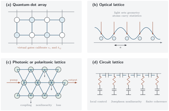
Four devices can implement a similar hopping graph while assigning different meanings to a site, particle, interaction, clock, and detector. A trustworthy comparison follows the full chain from fabricated graph through calibrated Hamiltonian and prepared state to measured observables.

The translation ledger

Platform	Site and particle	Principal coupling	Interaction	Natural readout
quantum-dot array	confined electronic orbital; fermionic electron or hole	gate-controlled tunnelling	charging, exchange, and longer-range Coulomb terms	charge sensing and electrical transport
optical lattice	Wannier orbital; bosonic or fermionic atom	wavefunction tunnelling	contact, dipolar, or mediated interaction	time of flight, spectroscopy, or site-resolved imaging
photonic lattice	waveguide, ring, or cavity mode; optical field or photon	evanescent or resonant coupling	often negligible; Kerr, emitter-mediated, or excitonic when engineered	output intensity, phase, spectrum, and correlations
polariton lattice	microcavity mode; mixed photon–exciton boson	photon hopping plus excitonic hybridization	exciton-mediated nonlinearity and saturation	angle-, energy-, time-, and position-resolved emission
circuit lattice	resonator or nonlinear circuit mode; microwave photon or encoded excitation	capacitive, inductive, or parametrically activated exchange	Josephson anharmonicity and engineered couplers	site-resolved microwave readout and state tomography

The table is a translation, not an equivalence proof. Matching the intended $J_{ij}$ does not establish matching statistics, interactions, reservoirs, preparation, or measurement operators.

Quantum-Dot Arrays

From artificial atoms to an extended Hubbard array

For one active orbital per dot, a common fermionic model is

$$\begin{aligned} H_{\mathrm{QD}} ={}& H_{\epsilon} + H_t + H_C, \\ H_{\epsilon} ={}& \sum_{i,\sigma} \widetilde{\epsilon}_i n_{i\sigma}, \\ H_t ={}& - \sum_{\langle i,j\rangle,\sigma} \left( t_{ij} d_{i\sigma}^{\dagger}d_{j\sigma} + \mathrm{h.c.} \right), \\ H_C ={}& \sum_i U_i n_{i\uparrow}n_{i\downarrow} + \sum_{i<j} V_{ij}n_i n_j . \end{aligned}$$

The onsite energy $\widetilde{\epsilon}_i$ includes gate voltages, static disorder, and the electrostatic shifts caused by occupation elsewhere in the array. The offsite terms $V_{ij}$ are often appreciable because Coulomb interactions are long ranged. A minimal onsite-only Hubbard model is therefore a hypothesis to test, not a default consequence of drawing an array of dots.

Gate voltages are not local coordinates. To first order,

$$\delta\boldsymbol{\epsilon} = \mathbf A\, \delta\mathbf V_{\mathrm g},$$

where the lever-arm matrix $\mathbf A$ is generally dense. Experimental virtual gates apply an approximate inverse of this matrix so that one control coordinate changes a chosen onsite energy or barrier while compensating crosstalk. The inverse is only local in parameter space: charge rearrangements and gate-dependent capacitances require recalibration.

In the singly occupied, large-interaction regime, virtual hopping produces antiferromagnetic exchange. For a symmetric two-site sector with nearest-neighbor repulsion,

$$J_{\mathrm{ex}} \simeq \frac{4|t|^2}{U-V}, \qquad |t|\ll U-V.$$

This relation is a useful scale estimate, but it does not certify a Heisenberg array. Valley states, spin–orbit coupling, direct exchange, charge admixture, and unequal dot energies can change the effective spin Hamiltonian.

What experiments have established

Gate-defined arrays have demonstrated homogeneous tuning and a collective Coulomb-blockade crossover in a finite Fermi–Hubbard chain. Calling that crossover a finite-size analog of a Mott transition is precise; calling it a thermodynamic Mott phase would overstate the evidence. Atomically patterned dopant arrays have reached two-dimensional $3\times3$ devices with extended interactions, while their reported disorder leaves uncertainty in the inferred Hamiltonian. Four-dot germanium devices have prepared and probed resonating-valence-bond correlations, and shared-control architectures have operated sixteen-dot arrays, showing substantial progress in control scaling.

The central obstacle is not merely fabricating more dots. A many-body simulator requires simultaneous evidence for:

• a known charge sector and active orbital on every site;
• calibrated onsite energies, tunnel amplitudes, and cross-capacitances;
• temperatures below the exchange or correlation scale of interest;
• readout that distinguishes local occupation and spin correlations;
• stability over the complete acquisition and calibration interval;
• an uncertainty model for disorder and omitted long-range terms.

Transport through the entire array can be dominated by contacts or bottlenecks. Agreement between one conductance trace and one Hubbard calculation is therefore weaker than agreement across charge sensing, excitation spectroscopy, parameter sweeps, and held-out correlation observables.

Optical Lattice Analogs

Clean potentials do not guarantee cold many-body states

Interfering laser fields create periodic potentials whose lowest-band projection can realize Bose–Hubbard, Fermi–Hubbard, spin, and synthetic-gauge models. The detailed construction and Wannier integrals are developed in Optical Lattices. In the simplest single-band case,

$$\begin{aligned} H_{\mathrm{atom}} ={}& H_J + H_U + H_{\mathrm{trap}}, \\ H_J ={}& - \sum_{\langle i,j\rangle,\sigma} \left( J_{ij} e^{i\phi_{ij}} a_{i\sigma}^{\dagger}a_{j\sigma} + \mathrm{h.c.} \right), \\ H_U ={}& \sum_i \frac{U_i}{2} n_i(n_i-1), \\ H_{\mathrm{trap}} ={}& \sum_i V_i^{\mathrm{trap}}n_i . \end{aligned}$$

The platform’s strengths are low microscopic disorder, controllable statistics and interactions, flexible geometry, and isolation from a solid-state bath. Quantum gas microscopy can measure occupation and correlations site by site. Periodic driving and laser-assisted tunnelling can add Peierls phases and synthetic flux.

Its limiting resources are preparation entropy, slow equilibration, particle loss, residual harmonic confinement, calibration of $J/U$, and heating from lattice light or drive. A visually uniform optical potential need not produce a homogeneous state because the smooth trap changes the local chemical potential. Likewise, a slow lattice ramp relative to a band gap can still be nonadiabatic relative to a small many-body gap.

An evidence ladder from model to phase

The bosonic superfluid–Mott transition, site-resolved atomic Mott plateaus, the Floquet Haldane band, and long-range antiferromagnetic correlations in a finite two-dimensional Fermi–Hubbard system are landmark demonstrations at different rungs of the ladder. They should not be compressed into one statement that “optical lattices solve the Hubbard model.”

For a phase-level claim, report:

1. the calibrated lattice geometry, depth, hopping, interaction, and trap;
2. filling and entropy or a validated thermometer;
3. higher-band population and heating versus hold time;
4. the detector’s parity, spin, and loss response;
5. spatial correlations and finite-size dependence, not only an averaged density;
6. comparison with at least one competing Hamiltonian or omitted term.

The simulator reproduces selected observables of a model. It does not automatically reproduce phonons, Coulomb tails, orbital chemistry, or electrical transport in the material that motivated that model.

Photonic and Polaritonic Lattices

Propagation can emulate time

In a weakly guiding waveguide array, the paraxial equation maps longitudinal propagation to Schrödinger evolution. After a modal projection,

$$i\frac{d\boldsymbol{\psi}}{dz} = \mathbf K(z)\boldsymbol{\psi},$$

where $z$ is a propagation coordinate and $\mathbf K$ is a coupling matrix. This mapping makes waveguide arrays exceptionally direct laboratories for interference, edge propagation, Floquet band engineering, and compact localized states. It does not turn an optical beam into an equilibrium electron gas: the observed output is the propagated field from a chosen input condition.

Ring resonators, photonic crystals, and cavity arrays instead evolve in laboratory time. A semiclassical driven array often obeys

$$\begin{aligned} i\frac{d\alpha_i}{dt} ={}& \left( \omega_i - i\frac{\kappa_i}{2} \right) \alpha_i - \sum_j J_{ij}\alpha_j \\ & + U_i|\alpha_i|^2\alpha_i + F_i(t). \end{aligned}$$

Here the linewidth $\kappa_i$, pump $F_i$, and nonlinear shift $U_i|\alpha_i|^2$ affect the measured spectrum and spatial pattern. For few-photon claims, the operator master equation and normally ordered correlation functions are required; a classical coupled-mode fit is insufficient.

Exciton–polaritons add a matter fraction that strengthens interactions but also introduces exciton disorder, saturation, reservoir dynamics, and branch-dependent loss. Their emitted light provides unusually rich momentum- and position-resolved access to the mode, while simultaneously making the detector part of an open-system inference problem. Driven-Dissipative Matter owns the pump–loss field theory and the distinction among condensation, lasing, and superfluid response.

What topological photonics demonstrates

Coupled silicon rings and helical waveguide arrays have demonstrated boundary-localized propagation robust against selected defects. Photonic Lieb lattices have displayed compact flat-band localization. Polariton honeycomb lattices have resolved Dirac cones and flat bands, and magnetically biased polariton lattices have shown chiral edge-mode propagation and reversal with field.

These are substantive topological-wave and band-engineering results. They do not imply quantized electronic Hall conductance, a filled Fermi sea, or immunity to arbitrary disorder. A strong topological claim should connect:

• a calibrated bulk coupling model to a bulk gap;
• boundary spectroscopy to modes traversing that gap;
• propagation or scattering to a stated class of defects;
• the measured mode structure to a bulk invariant or equivalent dynamical diagnostic;
• loss, gain, nonlinearity, and non-Hermiticity to the model used for the invariant.

“Light went around a corner” is evidence for guided boundary transport, not by itself a measurement of a Chern number.

Circuit Lattices

Josephson nonlinearity makes photons interact

Arrays of superconducting resonators, transmons, or hybrid qubit–resonator cells can implement bosonic hopping models with strong, adjustable nonlinearities. A useful rotating-frame model is

$$\begin{aligned} \frac{H_{\mathrm{circ}}}{\hbar} ={}& \sum_i \left[ \Delta_i n_i + \frac{K_i}{2} n_i(n_i-1) \right] \\ & - \sum_{i\ne j} \left( J_{ij}e^{i\phi_{ij}} b_i^\dagger b_j + \mathrm{h.c.} \right) \\ & + \frac{H_{\mathrm{pump}}}{\hbar}. \end{aligned}$$

The Josephson element supplies the Kerr scale $K_i$ or an effective spin nonlinearity. Tunable couplers and parametric modulation control $J_{ij}$ and can imprint synthetic Peierls phases. Microwave control enables local preparation and time-resolved measurement inaccessible in most natural materials.

The same components create limitations: fabrication spread in $\Delta_i$, leakage beyond a qubit subspace, drive-induced Stark shifts, residual couplings, correlated control errors, relaxation, and dephasing. The useful dynamical window must satisfy

$$\begin{aligned} \Gamma_{\mathrm{inc}} &\equiv \max_i \left\{ \kappa_i,\gamma_{\phi i} \right\}, \\ \hbar\Gamma_{\mathrm{inc}} &\ll E_{\mathrm{dyn}}, \\ \tau_{\mathrm{sequence}} \Gamma_{\mathrm{inc}} &\ll 1, \end{aligned}$$

unless dissipation is intentionally included in the target.

Small superconducting circuits have measured chiral currents of interacting microwave photons under synthetic flux. Larger circuit-QED chains have revealed driven dissipative switching and spectroscopic signatures of localization. Reservoir engineering has stabilized an incompressible one-photon-per-site state and followed defect removal in a Bose–Hubbard array. The phrase “Mott insulator of photons” in that experiment refers to a deliberately stabilized open-system state; it should not be silently reinterpreted as the equilibrium ground state of a closed photon-number-conserving solid.

Designer Flat Bands and Topology

Geometry is a control knob, not a conclusion

Lieb, kagome, stub, dice, and line-graph geometries can suppress dispersion through destructive interference. Honeycomb and dimerized graphs can host Dirac crossings or topological band inversions. Artificial platforms are valuable because bonds and boundaries can be changed without synthesizing an entirely new bulk crystal.

The gauge-invariant flux through an oriented loop $\mathcal C$ is

$$\Phi_{\mathcal C} = \left[ \sum_{(ij)\in\mathcal C} \phi_{ij} \right]_{\!2\pi}.$$

Individual bond phases depend on the site basis; loop fluxes do not. A topological design therefore requires phase calibration around independent loops, not merely a programmed waveform that was intended to create complex hopping.

The term flat band also needs an operational definition. Measure the full relevant dispersion and quote its bandwidth $W$, isolation gap $\Delta_{\mathrm{iso}}$, linewidth or disorder scale $\Gamma$, interaction scale $U_{\mathrm{eff}}$, and temperature. A density-of-states peak or a localized input pattern is not enough to determine all five. The canonical distinctions among spectral flatness, compact states, quantum geometry, and correlated Chern bands are developed in Flat Bands.

Atom-by-atom and electrostatic electronic lattices

Scanning-probe manipulation of repulsive CO molecules on Cu(111) has confined surface-state electrons into artificial honeycomb, Lieb, and fractal geometries. Spectroscopy and wavefunction maps established designer Dirac behavior, a Lieb-lattice flat band, and geometry-dependent fractal electronic states. These experiments offer atomic control and direct local spectroscopy, but the substrate continuum, finite structures, tip response, and weak interaction scale delimit the analogy to an isolated many-body lattice.

Electrostatically patterned two-dimensional electron gases provide a complementary route with transport access and Coulomb interactions. As of this review, a low-disorder, gate-defined GaAs artificial crystal has reported tunable graphene-like and kagome-like bands together with a correlated insulating state near the kagome flat band. That is an important recent active result; reproducing its gap, order, and scaling across devices and probes will determine how broadly the phase assignment holds.

The designer-matter claim ladder

Claim	Minimum evidence
fabricated graph	structural image, site count, boundary, and defect inventory
one-body lattice	calibrated onsite terms and links; measured modes or dispersion agree within uncertainty
synthetic gauge field	loop phases or a gauge-invariant dynamical response
interacting model	independently constrained interaction scale and a correlation observable not fit by the one-body model
many-body state	filling, temperature or steady-state distribution, correlations, and alternatives tested
phase	order parameter, invariant, gap, or response plus size, time, and robustness evidence appropriate to the definition
computational advantage	a well-defined task, verified outputs where possible, uncertainty, and evidence against the best relevant classical methods

Programmability strengthens causal tests because one can vary a single Hamiltonian term and predict the response. It does not remove the need to calibrate what the controls actually did.

A Cross-Platform Validation Protocol

Seven contracts

Before interpreting an artificial lattice, close seven contracts:

1. Active-space contract: identify the physical modes retained as sites and bound leakage to all omitted modes.
2. Graph contract: verify intended links, absent links, boundaries, and connectivity defects.
3. Parameter contract: calibrate onsite energies, hopping magnitudes and phases, interactions, and their covariance.
4. State contract: specify preparation, filling, entropy or distribution, and reproducibility.
5. open-system contract: measure heating, loss, dephasing, pump, and reservoir memory over the observation window.
6. detector contract: reconstruct which operator or correlation function the instrument measures, including its response matrix.
7. prediction contract: test held-out observables and parameter regimes rather than only the data used to infer the model.

A compact error budget can be organized around a relevant target scale $E_\star$:

$$\begin{aligned} \varepsilon_{\mathrm{impl}} &= \max \left\{ \varepsilon_{\mathrm{cal}}, \varepsilon_{\mathrm{leak}}, \varepsilon_{\mathrm{open}}, \varepsilon_T \right\}, \\ \varepsilon_{\mathrm{cal}} &= \frac{\lVert\delta H_{\mathrm{cal}}\rVert}{E_\star}, \\ \varepsilon_{\mathrm{leak}} &= \frac{\lVert\delta H_{\mathrm{leak}}\rVert}{E_\star}, \\ \varepsilon_{\mathrm{open}} &= \frac{\hbar\Gamma_{\mathrm{unwanted}}}{E_\star}, \\ \varepsilon_T &= \frac{k_{\mathrm B}T_{\mathrm{eff}}}{E_\star}. \end{aligned}$$

This is not a universal fidelity metric. It forces each nuisance into comparable units and exposes which assumption controls the claimed regime. In a deliberately open simulator, replace $\Gamma_{\mathrm{unwanted}}$ by uncertainty in the target dissipator and replace $T_{\mathrm{eff}}$ when no thermal description applies.

Platform comparison

Platform	Strongest leverage	Dominant nuisance	Especially strong evidence	A common overclaim
quantum dots	electrical tuning and genuine fermions	electrostatic disorder and crosstalk	charge-sector maps plus local correlations	finite blockade crossover called a bulk Mott transition
optical lattices	clean geometry, statistics, and interaction control	entropy, trap inhomogeneity, heating	site-resolved density and spin correlations	target Hamiltonian assumed to imply its ground state
photonics	direct mode imaging and long designed graphs	weak interactions, loss, input dependence	bulk and edge spectroscopy with phase-resolved propagation	optical edge guidance equated with quantized electron transport
polaritons	band imaging plus appreciable nonlinearity	reservoir, saturation, disorder, finite lifetime	energy–momentum tomography and pump-dependent dynamics	condensation equated with equilibrium superfluidity
circuits	local quantum control, strong nonlinearity, tomography	decoherence, fabrication spread, leakage	time-domain correlations and calibrated state populations	a prepared small-system eigenstate called a thermodynamic phase
assembled surface lattices	atomic geometry and local spectroscopy	substrate continuum and finite size	structural registration plus energy-resolved wavefunction maps	a spectral feature treated as interacting order

The best platform depends on the observable. There is no platform-independent ranking of “quantum simulation quality.”

Common Mistakes

Equating the graph with the Hamiltonian

A photograph establishes geometry. It does not establish hopping amplitudes, phases, interactions, statistics, or reservoirs.

Calling every incompressible signal a Mott state

Single-particle gaps, Coulomb blockade, disorder localization, band insulation, and driven number stabilization can all reduce compressibility. The mechanism and finite-size status must be identified.

Using linewidth as bandwidth

Bandwidth is dispersion across momentum or modes. Linewidth is spectral broadening at a mode. Disorder can broaden an ensemble while each local resonance remains narrow.

Treating photons as charge carriers

Photonic topology can reproduce wave equations, invariants, and boundary propagation. It does not inherit a Fermi level or quantized electrical conductance.

Ignoring preparation because the Hamiltonian is calibrated

A faithful Hamiltonian can be initialized in a hot, excited, or metastable state. Hamiltonian validation and state validation are separate.

Removing drive and loss from an open-system claim

In photonic, polaritonic, and many circuit experiments, pump and dissipation select the steady state. Treating them as small corrections can change the problem being claimed.

Extrapolating a finite array without a scaling variable

A gap or correlation measured on a few sites may be real and scientifically useful. Calling it a phase requires a definition and evidence for behavior with system size, correlation length, or an appropriate finite-system invariant.

Assuming programmability means independent control

Shared electrodes, optical aberrations, parametric sidebands, and microwave crosstalk correlate nominal controls. The calibrated control matrix, not the number of software knobs, determines independence.

Practical Interpretation Workflow

1. Name the target. Give the Hamiltonian, particle statistics, conserved quantities, boundary conditions, and intended observable.
2. Name the implementation. Identify physical sites, links, interactions, drives, reservoirs, and detector.
3. Measure the graph. Verify missing, unintended, and boundary links rather than relying only on design files.
4. Calibrate locally and globally. Determine parameter matrices and then test collective spectra or dynamics.
5. Bound leakage. Vary energy, drive, occupation, and time to expose higher orbitals, bands, or circuit levels.
6. Characterize the state. Report filling, entropy or distribution, correlations, and preparation fidelity.
7. Close the lifetime budget. Compare coherent, interaction, preparation, measurement, heating, and loss times.
8. Validate the detector. State the measured operator and invert detector response only with uncertainty propagation.
9. Test a withheld prediction. Change a parameter not used in calibration and predict a new spectrum, correlator, or trajectory.
10. Use the narrowest justified noun. Prefer “finite-size analog,” “band realization,” or “driven steady state” when “phase” is not established.

Exercises

1. Gauge transformations and loop flux

Let the site operators transform as $c_i\mapsto e^{i\chi_i}c_i$. Show how a hopping phase $\phi_{ij}$ transforms and prove that $\Phi_{\mathcal C}$ is unchanged around a closed oriented loop.

Solution

The hopping operator transforms as

$$c_i^\dagger c_j \longmapsto e^{-i\chi_i} e^{i\chi_j} c_i^\dagger c_j.$$

The same Hamiltonian form is retained if

$$\phi_{ij} \longmapsto \phi_{ij} + \chi_i - \chi_j.$$

Summing around the loop gives

$$\sum_{(ij)\in\mathcal C} \left( \phi_{ij} + \chi_i - \chi_j \right) = \sum_{(ij)\in\mathcal C} \phi_{ij},$$

because every site phase appears once with each sign. The loop flux modulo $2\pi$ is therefore gauge invariant, even though no individual bond phase is.

2. Exchange scale in a double dot

A symmetric double dot has $U=1.20\,\mathrm{meV}$, nearest-neighbor repulsion $V=0.20\,\mathrm{meV}$, and $|t|=30\,\mu\mathrm{eV}$. Estimate $J_{\mathrm{ex}}$ and check the small-hopping condition.

Solution

The virtual charge-excitation cost is

$$U-V = 1.00\,\mathrm{meV}.$$

Therefore

$$\begin{aligned} J_{\mathrm{ex}} &\simeq \frac{4(0.030\,\mathrm{meV})^2} {1.00\,\mathrm{meV}} \\ &= 0.0036\,\mathrm{meV} = 3.6\,\mu\mathrm{eV}. \end{aligned}$$

The ratio $|t|/(U-V)=0.03$ is small, so the leading second-order estimate is plausible. It would still need corrections for detuning, valley states, spin–orbit coupling, and higher orbitals in a real device.

3. Diagnose a finite-size insulator claim

A six-site dot chain shows a conductance minimum at one electron per site. The minimum deepens as $U/t$ increases, but no local charge sensor or temperature estimate is available. Which claim level is supported, and what three measurements would most improve it?

Solution

The data support an interaction-dependent transport suppression in a finite array. They are compatible with collective Coulomb blockade or a finite-size Mott analog, but they do not establish uniform filling, bulk incompressibility, or a thermodynamic phase.

The most useful additions are:

1. site-resolved or sufficiently local charge sensing to establish the occupation pattern;
2. compressibility or addition spectroscopy showing an interaction gap rather than a contact bottleneck;
3. calibrated electron temperature and a parameter sweep comparing the gap with $t$, $U$, and disorder.

Repeating the measurement for several chain lengths and contact configurations would then address scaling and lead effects.

4. Coherent cycles in a circuit lattice

A circuit lattice has $J/(2\pi)=20\,\mathrm{MHz}$, Kerr nonlinearity $|K|/(2\pi)=100\,\mathrm{MHz}$, and photon-loss rate $\kappa/(2\pi)=1.0\,\mathrm{MHz}$. Compute $|K|/J$, $\kappa/J$, and the number of hopping periods $2\pi/J$ within one lifetime $1/\kappa$.

Solution

Ratios are unchanged when all angular frequencies are divided by $2\pi$:

$$\frac{|K|}{J} = 5, \qquad \frac{\kappa}{J} = 0.05.$$

The hopping period is $2\pi/J=1/(20\,\mathrm{MHz})=50\,\mathrm{ns}$, while the lifetime is $1/\kappa=1/(2\pi\times1\,\mathrm{MHz})\simeq159\,\mathrm{ns}$. Thus

$$\frac{1/\kappa}{2\pi/J} = \frac{J}{2\pi\kappa} \simeq 3.18.$$

Only about three hopping periods fit within one lifetime. The energy ratio $\kappa/J=0.05$ can look small while the available real-time propagation window remains short; the convention for rates and periods matters.

5. A compact state on a Lieb plaquette

Four edge sites surround a connector site. Each edge couples to the connector with equal real hopping $J$. Construct amplitudes on the four edge sites that have equal magnitude, vanish on the connector, and cancel the net hopping into it.

Solution

Choose alternating amplitudes

$$\boldsymbol{\psi}_{\mathrm{edge}} = \frac{1}{2} \left( 1,-1,1,-1 \right).$$

The amplitude driven onto the connector is proportional to

$$J \sum_{\ell=1}^{4} \psi_\ell = \frac{J}{2} \left( 1-1+1-1 \right) = 0.$$

Destructive interference therefore isolates this pattern from the connector in the ideal equal-link model. Unequal couplings, onsite disorder, next-neighbor hopping, or loss imbalance generally spoil exact compactness. Observing localization from this input tests interference, but a full flat-band claim still requires the mode spectrum or dispersion.

6. Design a held-out validation test

A photonic array’s onsite frequencies and nearest-neighbor couplings were fitted to its transmission spectrum. Propose one held-out measurement that is sensitive to an omitted next-nearest-neighbor hopping $J_2$ and explain why refitting the original spectrum is weaker.

Solution

One can inject a localized wavepacket with controlled momentum content and predict its phase-resolved propagation to several output distances using the fitted nearest-neighbor model. Next-nearest-neighbor hopping changes the dispersion away from the originally resolved resonances and therefore shifts group velocities, interference nodes, or revival times. Alternatively, one can fabricate a boundary whose edge dispersion is first-order sensitive to $J_2$ and measure it without changing the fit.

Refitting the original spectrum is weaker because onsite shifts and nearest-neighbor couplings may absorb part of the $J_2$ effect. A held-out observable tests predictive structure that was not used to choose the parameters.

Research Status

• Established: programmable one-body graphs; many calibrated tight-binding dispersions; atomic Bose–Hubbard Mott states; cold-atom antiferromagnetic correlations; photonic and polaritonic edge and flat-band modes; finite circuit and dot Hubbard dynamics.
• Active: homogeneous two-dimensional fermionic dot arrays; equilibrium-scale interacting photon matter; scalable synthetic gauge fields with strong interactions; correlated electrostatic flat-band crystals; reliable finite-size-to-phase inference.
• Conjectural: that a given platform will outperform controlled classical methods on a scientifically decisive many-body observable before calibration uncertainty dominates.
• Speculative: broad claims that arbitrary materials can be replaced by programmable arrays or that topological band engineering alone guarantees useful, lossless devices.

Terminology varies across communities. “Simulation,” “emulation,” “realization,” “phase,” and “topological protection” should be read through the explicit evidence supplied, not treated as standardized certification labels.

Connections

• Tight-Binding Models develops orbital embeddings, Bloch matrices, hopping range, and Wannier representations.
• Hubbard Physics in Materials gives the active-space and model-discrimination workflow for natural solids.
• Quantum Dots and Coulomb Blockade own the charging and transport foundations of dot arrays.
• Optical Lattices derives optical potentials, recoil scales, Hubbard projection, loading, and calibration.
• Circuit QED Overview develops transmon and resonator hardware; Open-System Circuit QED develops measurement and dissipation.
• Flat Bands owns compact states, projector geometry, interaction projection, and Chern-band quality.
• Chern Numbers in Band Theory supplies the bulk invariant behind many designer topological bands.
• Floquet Quantum Matter develops quasienergy, micromotion, heating, and driven-topology validation.
• Driven-Dissipative Matter owns pump–loss steady states, polariton fluids, and open-system transition evidence.
• Engineered Heterostructures compares property transfer across physical interfaces rather than graph-programmed simulators.
• Quantum Materials by Design contrasts programmable emulation with the computation–synthesis–validation loop for natural and engineered compounds.

Further Reading

• I. M. Georgescu, S. Ashhab, and F. Nori, “Quantum Simulation,” Reviews of Modern Physics 86, 153–185 (2014), for a broad taxonomy of analog and digital simulation.
• I. Bloch, J. Dalibard, and W. Zwerger, “Many-Body Physics with Ultracold Gases,” Reviews of Modern Physics 80, 885–964 (2008), for optical-lattice many-body foundations.
• A. A. Houck, H. E. Türeci, and J. Koch, “On-Chip Quantum Simulation with Superconducting Circuits,” Nature Physics 8, 292–299 (2012), for circuit-lattice proposals and architecture.
• T. Ozawa et al., “Topological Photonics,” Reviews of Modern Physics 91, 015006 (2019), for the scope and limitations of topological-wave analogies.
• C. R. Ast et al., “Creating Designer Quantum States of Matter Atom-by-Atom,” Nature Reviews Physics 1, 703–715 (2019), for scanning-probe assembly of electronic and spin lattices.

References

1. R. P. Feynman, “Simulating Physics with Computers,” International Journal of Theoretical Physics 21, 467–488 (1982), doi:10.1007/BF02650179.
2. I. M. Georgescu, S. Ashhab, and F. Nori, “Quantum Simulation,” Reviews of Modern Physics 86, 153–185 (2014), doi:10.1103/RevModPhys.86.153.
3. T. Hensgens et al., “Quantum Simulation of a Fermi–Hubbard Model Using a Semiconductor Quantum Dot Array,” Nature 548, 70–73 (2017), doi:10.1038/nature23022.
4. X. Wang et al., “Experimental Realization of an Extended Fermi-Hubbard Model Using a 2D Lattice of Dopant-Based Quantum Dots,” Nature Communications 13, 6824 (2022), doi:10.1038/s41467-022-34220-w.
5. C.-A. Wang et al., “Probing Resonating Valence Bonds on a Programmable Germanium Quantum Simulator,” npj Quantum Information 9, 58 (2023), doi:10.1038/s41534-023-00727-3.
6. F. Borsoi et al., “Shared Control of a 16 Semiconductor Quantum Dot Crossbar Array,” Nature Nanotechnology 19, 21–27 (2024), doi:10.1038/s41565-023-01491-3.
7. D. Jaksch, C. Bruder, J. I. Cirac, C. W. Gardiner, and P. Zoller, “Cold Bosonic Atoms in Optical Lattices,” Physical Review Letters 81, 3108–3111 (1998), doi:10.1103/PhysRevLett.81.3108.
8. M. Greiner, O. Mandel, T. Esslinger, T. W. Hänsch, and I. Bloch, “Quantum Phase Transition from a Superfluid to a Mott Insulator in a Gas of Ultracold Atoms,” Nature 415, 39–44 (2002), doi:10.1038/415039a.
9. I. Bloch, J. Dalibard, and W. Zwerger, “Many-Body Physics with Ultracold Gases,” Reviews of Modern Physics 80, 885–964 (2008), doi:10.1103/RevModPhys.80.885.
10. W. S. Bakr, J. I. Gillen, A. Peng, S. Fölling, and M. Greiner, “A Quantum Gas Microscope for Detecting Single Atoms in a Hubbard-Regime Optical Lattice,” Nature 462, 74–77 (2009), doi:10.1038/nature08482.
11. J. F. Sherson et al., “Single-Atom-Resolved Fluorescence Imaging of an Atomic Mott Insulator,” Nature 467, 68–72 (2010), doi:10.1038/nature09378.
12. L. Tarruell et al., “Creating, Moving and Merging Dirac Points with a Fermi Gas in a Tunable Honeycomb Lattice,” Nature 483, 302–305 (2012), doi:10.1038/nature10871.
13. G. Jotzu et al., “Experimental Realization of the Topological Haldane Model with Ultracold Fermions,” Nature 515, 237–240 (2014), doi:10.1038/nature13915.
14. A. Mazurenko et al., “A Cold-Atom Fermi–Hubbard Antiferromagnet,” Nature 545, 462–466 (2017), doi:10.1038/nature22362.
15. M. Hafezi, S. Mittal, J. Fan, A. Migdall, and J. M. Taylor, “Imaging Topological Edge States in Silicon Photonics,” Nature Photonics 7, 1001–1005 (2013), doi:10.1038/nphoton.2013.274.
16. M. C. Rechtsman et al., “Photonic Floquet Topological Insulators,” Nature 496, 196–200 (2013), doi:10.1038/nature12066.
17. T. Jacqmin et al., “Direct Observation of Dirac Cones and a Flatband in a Honeycomb Lattice for Polaritons,” Physical Review Letters 112, 116402 (2014), doi:10.1103/PhysRevLett.112.116402.
18. S. Mukherjee et al., “Observation of a Localized Flat-Band State in a Photonic Lieb Lattice,” Physical Review Letters 114, 245504 (2015), doi:10.1103/PhysRevLett.114.245504.
19. F. Baboux et al., “Bosonic Condensation and Disorder-Induced Localization in a Flat Band,” Physical Review Letters 116, 066402 (2016), doi:10.1103/PhysRevLett.116.066402.
20. S. Klembt et al., “Exciton–Polariton Topological Insulator,” Nature 562, 552–556 (2018), doi:10.1038/s41586-018-0601-5.
21. T. Ozawa et al., “Topological Photonics,” Reviews of Modern Physics 91, 015006 (2019), doi:10.1103/RevModPhys.91.015006.
22. A. A. Houck, H. E. Türeci, and J. Koch, “On-Chip Quantum Simulation with Superconducting Circuits,” Nature Physics 8, 292–299 (2012), doi:10.1038/nphys2251.
23. P. Roushan et al., “Chiral Ground-State Currents of Interacting Photons in a Synthetic Magnetic Field,” Nature Physics 13, 146–151 (2017), doi:10.1038/nphys3930.
24. M. Fitzpatrick, N. M. Sundaresan, A. C. Y. Li, J. Koch, and A. A. Houck, “Observation of a Dissipative Phase Transition in a One-Dimensional Circuit QED Lattice,” Physical Review X 7, 011016 (2017), doi:10.1103/PhysRevX.7.011016.
25. P. Roushan et al., “Spectroscopic Signatures of Localization with Interacting Photons in Superconducting Qubits,” Science 358, 1175–1179 (2017), doi:10.1126/science.aao1401.
26. R. Ma et al., “A Dissipatively Stabilized Mott Insulator of Photons,” Nature 566, 51–57 (2019), doi:10.1038/s41586-019-0897-9.
27. K. K. Gomes et al., “Designer Dirac Fermions and Topological Phases in Molecular Graphene,” Nature 483, 306–310 (2012), doi:10.1038/nature10941.
28. M. R. Slot et al., “Experimental Realization and Characterization of an Electronic Lieb Lattice,” Nature Physics 13, 672–676 (2017), doi:10.1038/nphys4105.
29. S. N. Kempkes et al., “Design and Characterization of Electrons in a Fractal Geometry,” Nature Physics 15, 127–131 (2019), doi:10.1038/s41567-018-0328-0.
30. D. Leykam, A. Andreanov, and S. Flach, “Artificial Flat Band Systems: From Lattice Models to Experiments,” Advances in Physics: X 3, 1473052 (2018), doi:10.1080/23746149.2018.1473052.
31. O. Klochan et al., “Correlated Insulator in the Kagome Flat Band of a Two-Dimensional Electrostatic Crystal,” Nature Physics (2026), doi:10.1038/s41567-026-03291-7.