Circuit QED Overview

Circuit quantum electrodynamics, or circuit QED, couples quantized electromagnetic modes to fabricated quantum circuits. It borrows the language of atomic cavity QED but changes the physical implementation:

• a Josephson circuit replaces a natural atom;
• a coplanar, lumped-element, or three-dimensional microwave resonator replaces an optical cavity;
• coaxial lines and lithographic transmission lines replace free-space optical beams;
• cryogenic microwave sources replace lasers;
• quadrature receivers and parametric amplifiers replace optical photodetectors; and
• electromagnetic design makes many Hamiltonian parameters tunable rather than fixed by nature.

The analogy is powerful because the same bosonic modes, Rabi drives, Jaynes–Cummings interactions, dispersive shifts, input–output relations, and continuous measurements reappear. It is incomplete because an artificial atom is a nonlinear electrical oscillator with many levels, not an isolated two-level atom. Its control ports are also dissipation channels, its material interfaces can limit coherence, and its readout record is produced by an entire cryogenic receiver chain.

This overview is for readers who already know AMO quantum optics and want to understand what a circuit-QED experiment physically contains, which approximations connect it to familiar models, and what evidence supports a hardware-level claim.

Canonical Scope

Jaynes–Cummings Model owns the exact two-level, one-mode spectrum and coherent exchange dynamics. Cavity QED owns the universal $g$–$\kappa$–$\gamma$ theory, cooperativity, Purcell physics, and lossy spectra. Input–Output Theory Overview owns port boundary conditions and scattering conventions.

The open-system circuit-QED page owns master equations, measurement-induced dephasing, stochastic trajectories, and adiabatic elimination of the readout resonator. Josephson Effect is the canonical home for junction current–phase and voltage–phase relations, RCSJ dynamics, SQUID interference, and the bridge to circuit nonlinearity.

This page owns the platform layer:

• how linear circuits become microwave quantum modes;
• how Josephson nonlinearity produces artificial atoms;
• transmon energy scales and the controlled two-level truncation;
• microwave resonator, package, port, and cryogenic architectures;
• how the Jaynes–Cummings analogy changes for a multilevel circuit;
• dispersive-readout hardware and calibration;
• the relation between circuit QED and processor control;
• platform-specific noise, leakage, crosstalk, and thermal budgets; and
• the evidence ledger needed to validate an experiment.

It does not attempt a microscopic theory of superconductivity, a complete circuit-quantization formalism, or a survey of every superconducting-qubit modality.

Translation from Atomic to Circuit QED

The correspondence is most useful when each abstract symbol is tied to a physical object.

Atomic or optical language	Circuit-QED realization	Important qualification
atomic transition	transition between eigenstates of a Josephson circuit	several nearby levels usually exist
optical cavity mode	standing microwave mode of a distributed or lumped resonator	package and slotline modes may also participate
dipole matrix element	charge- or flux-operator matrix element	set by circuit impedance and junction parameters
laser drive	phase-coherent microwave tone	synthesized, attenuated, filtered, and routed through a port
spontaneous emission	radiative and nonradiative relaxation	impedance and material participation matter
homodyne detection	microwave mixing against a local oscillator	amplification adds noise and finite bandwidth
cavity output coupler	coupling capacitor, pin, aperture, or transmission-line port	the same port can create Purcell decay
fixed species	fabricated circuit design	fabrication spread and drift require calibration

Natural atoms have precise selection rules and reproducible spectra. Artificial atoms offer larger electrical dipoles, lithographic integration, and tunability, but their finite anharmonicity makes leakage and drive-dependent dressing central engineering constraints.

From a Circuit to a Quantum Mode

Flux and charge as canonical variables

An electrical network becomes a quantum system after one identifies independent node-flux coordinates. For a node voltage $V(t)$, define

$$\Phi(t) = \int^t V(t')\,dt'.$$

The conjugate variable is the node charge $Q$. For one ideal $LC$ mode,

$$H_{LC} = \frac{Q^2}{2C} + \frac{\Phi^2}{2L}, \qquad [\Phi,Q] = i\hbar.$$

This is a harmonic oscillator with

$$\omega_r = \frac{1}{\sqrt{LC}}, \qquad Z_r = \sqrt{\frac{L}{C}}.$$

A convenient operator convention is

$$\begin{aligned} \Phi &= \Phi_{\mathrm{zpf}} \left( a+a^\dagger \right), \\ Q &= -iQ_{\mathrm{zpf}} \left( a-a^\dagger \right), \end{aligned}$$

where

$$\Phi_{\mathrm{zpf}} = \sqrt{\frac{\hbar Z_r}{2}}, \qquad Q_{\mathrm{zpf}} = \sqrt{\frac{\hbar}{2Z_r}}.$$

Thus impedance controls the size of vacuum flux and charge fluctuations. Large impedance enhances flux fluctuations; small impedance enhances charge fluctuations. This is the circuit counterpart of changing optical mode volume to alter a vacuum-field amplitude.

Why a linear circuit is not an atom

Every transition of an ideal $LC$ oscillator has the same frequency:

$$E_m = \hbar\omega_r \left( m+\frac12 \right).$$

A resonant control pulse therefore cannot select $|0\rangle\leftrightarrow |1\rangle$ without also addressing higher transitions. A qubit needs nonlinearity so that

$$\omega_{12} \neq \omega_{01}.$$

In superconducting circuits, the Josephson junction supplies a low-loss nonlinear inductive energy

$$U_J(\phi) = -E_J\cos\phi,$$

where $\phi$ is the gauge-invariant phase difference and

$$E_J = \frac{\hbar I_c}{2e}.$$

Expanding the cosine begins with a quadratic inductance and then produces quartic and higher nonlinearities:

$$-E_J\cos\phi = -E_J + \frac{E_J}{2}\phi^2 - \frac{E_J}{24}\phi^4 + \cdots.$$

The quadratic term joins the linear circuit; the higher terms make the spectrum anharmonic.

Artificial Atoms

The transmon Hamiltonian

The transmon is a capacitively shunted Josephson junction or split-junction loop. Its standard single-mode Hamiltonian is

$$H_{\mathrm t} = 4E_C \left( n-n_g \right)^2 - E_J\cos\phi,$$

with

$$[\phi,n] = i.$$

Here:

• $n$ counts excess Cooper-pair charge in units of $2e$;
• $n_g$ is the dimensionless offset charge;
• $E_C=e^2/(2C_\Sigma)$ is the charging energy for total island capacitance $C_\Sigma$; and
• $E_J$ is the Josephson energy.

The cosine makes $\phi$ a compact coordinate. The exact eigenproblem can be represented in the charge basis and solved numerically. In the transmon regime,

$$\frac{E_J}{E_C} \gg 1,$$

wavefunctions are localized near a minimum of the cosine potential. Charge dispersion becomes exponentially small in $\sqrt{E_J/E_C}$, making the transition frequency comparatively insensitive to offset-charge noise.

Weakly anharmonic spectrum

Expanding near $\phi=0$ and treating the quartic term perturbatively gives, to leading order,

$$\frac{\omega_{01}}{2\pi} \simeq \frac{\sqrt{8E_JE_C}-E_C}{h},$$

and

$$\frac{\alpha}{2\pi} \equiv \frac{\omega_{12}-\omega_{01}}{2\pi} \simeq -\frac{E_C}{h}.$$

The transmon is therefore only weakly anharmonic:

$$|\alpha| \ll \omega_{01}.$$

That is both a strength and a cost. Large $E_J/E_C$ suppresses charge sensitivity, while a small relative anharmonicity makes short control pulses more likely to populate $|2\rangle$ and higher states.

Worked transmon audit

Suppose

$$\frac{E_J}{h} = 20.0\ \mathrm{GHz}, \qquad \frac{E_C}{h} = 0.250\ \mathrm{GHz}.$$

Then

$$\frac{E_J}{E_C} = 80,$$

and the leading transmon approximation gives

$$\begin{aligned} \frac{\omega_{01}}{2\pi} &\simeq \sqrt{ 8(20.0)(0.250) } - 0.250 \\ &= 6.075\ \mathrm{GHz}. \end{aligned}$$

The anharmonicity and next transition are approximately

$$\frac{\alpha}{2\pi} \simeq -0.250\ \mathrm{GHz},$$ $$\frac{\omega_{12}}{2\pi} \simeq 5.825\ \mathrm{GHz}.$$

A measured spectrum should be compared with a numerical diagonalization, not only these asymptotic formulas. Junction asymmetry, additional modes, and coupling-induced Lamb shifts can move the transitions.

A qubit is a selected subspace

The computational states are usually the two lowest eigenstates,

$$|0\rangle \equiv |g\rangle, \qquad |1\rangle \equiv |e\rangle.$$

They do not exhaust the Hilbert space. A reliable control model retains enough levels to estimate leakage and drive-induced frequency shifts:

$$H_{\mathrm{atom}} = \sum_j \hbar\omega_j |j\rangle\langle j|.$$

The charge operator has adjacent-level matrix elements

$$n_{j,j+1} = \langle j|n|j+1\rangle$$

that grow approximately as $\sqrt{j+1}$ in the weakly anharmonic limit. Consequently, a tone aimed at $|0\rangle\leftrightarrow|1\rangle$ can off-resonantly drive $|1\rangle\leftrightarrow|2\rangle$.

Tunability and sweet spots

Replacing one junction by a superconducting loop containing two junctions makes an effective $E_J$ flux dependent. This permits frequency tuning and parametric interactions. Tunability also couples the transition frequency to flux noise. At a first-order sweet spot,

$$\frac{\partial\omega_{01}}{\partial\Phi_{\mathrm{ext}}} = 0,$$

small flux fluctuations contribute only at second and higher order. A frequency-tunable device therefore carries a control-versus-dephasing tradeoff absent from an ideal fixed atom.

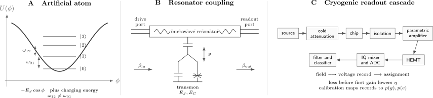
A circuit-QED platform is a cascade. A Josephson nonlinearity creates an anharmonic artificial atom; a microwave resonator mediates coupling and readout; attenuators, isolators, quantum-limited amplification, and room-temperature demodulation turn an outgoing field into a calibrated record. No one block alone determines control or measurement fidelity.

Microwave Resonators

Distributed coplanar resonators

A coplanar-waveguide resonator is a section of superconducting transmission line bounded by capacitive or inductive discontinuities. For phase velocity $v_p$ and physical length $\ell$, a half-wave mode has approximately

$$\omega_m \simeq (m+1) \frac{\pi v_p}{\ell}, \qquad m=0,1,2,\ldots.$$

The exact spectrum depends on boundary capacitances, bends, kinetic inductance, coupling structures, and loading by qubits. Distributed resonators offer spatially separated voltage antinodes, multiple ports, and bus modes that can connect several circuits.

Lumped-element resonators

An interdigitated or parallel-plate capacitor joined to a spiral or meandered inductor approximates a compact $LC$ mode. Lumped resonators can reduce footprint and make impedance easier to engineer, but stray capacitance and package coupling become a larger fraction of the intended circuit.

Three-dimensional cavities

A machined superconducting enclosure supports microwave modes with large physical volume and potentially small surface participation. A chip-mounted qubit couples through an antenna. Three-dimensional cavities can provide long-lived storage and clean mode structure, but they are less naturally dense than planar layouts and require careful package-mode accounting.

Readout, bus, and storage roles

Not every resonator should have the same linewidth.

• A readout resonator is deliberately coupled to an output line so its state-dependent field leaves quickly enough to measure.
• A bus resonator mediates coherent interactions between circuits and may be only virtually excited during a gate.
• A storage resonator is engineered for long photon lifetime and small internal loss.
• A Purcell filter is an additional frequency-selective network that passes readout photons while suppressing qubit-frequency radiation.

Calling every mode “the cavity” hides these distinct functions.

Linewidth and quality-factor conventions

Let $\kappa$ be the resonator energy-decay rate, so that

$$\frac{d}{dt} \langle a^\dagger a\rangle = -\kappa \langle a^\dagger a\rangle$$

without a drive. The field amplitude decays at $\kappa/2$. For a resonance with ordinary frequency $f_r=\omega_r/(2\pi)$ and full width at half maximum $\Delta f$, this convention gives

$$\Delta f = \frac{\kappa}{2\pi}, \qquad Q = \frac{\omega_r}{\kappa} = \frac{f_r}{\Delta f}.$$

Separate the total rate into ports and internal loss:

$$\kappa = \kappa_{\mathrm{in}} + \kappa_{\mathrm{out}} + \kappa_{\mathrm{int}} + \cdots.$$

The loaded, coupling, and internal quality factors obey

$$\frac{1}{Q_L} = \frac{1}{Q_{\mathrm{in}}} + \frac{1}{Q_{\mathrm{out}}} + \frac{1}{Q_i}.$$

One must state whether a quoted linewidth describes energy or field decay and whether it is angular or ordinary frequency.

A cryogenic electromagnetic environment

Microwave photons near several gigahertz have energies far below optical photons. Their equilibrium occupation at temperature $T$ is

$$\bar n_{\mathrm{th}} = \frac{1}{ \exp\!\left( \hbar\omega_r/k_{\mathrm B}T \right)-1 }.$$

For $f_r=6.0\ \mathrm{GHz}$,

$$\frac{hf_r}{k_{\mathrm B}} \simeq 0.288\ \mathrm K.$$

The equilibrium occupations are approximately

$$\begin{array}{c|c} T & \bar n_{\mathrm{th}}\\ \hline 20\ \mathrm{mK} & 5.6\times10^{-7}\\ 50\ \mathrm{mK} & 3.16\times10^{-3}\\ 100\ \mathrm{mK} & 5.95\times10^{-2} \end{array}$$

A dilution refrigerator base temperature does not prove that a mode has the corresponding occupation. Warm radiation can enter through a control line; attenuators can be poorly thermalized; nonequilibrium quasiparticles can excite a qubit; and amplifier backaction can propagate toward the device. Effective mode temperature is an inferred property, not a label copied from a thermometer.

Attenuation, filtering, and isolation

An input chain usually distributes attenuation among temperature stages so that room-temperature thermal noise is absorbed and re-emitted at progressively lower temperatures. Low-pass, infrared, and absorptive filters limit out-of-band radiation. Output isolators or circulators reduce noise sent back from amplifiers.

These components have finite insertion loss, bandwidth, magnetic-field sensitivity, and thermalization. A wiring diagram should therefore report where attenuation occurs, which ports are monitored, and which losses occur before the first amplifier.

Internal loss and participation

Resonator loss is frequently organized by participation ratios:

$$\frac{1}{Q_i} \simeq \sum_k p_k\tan\delta_k + \frac{1}{Q_{\mathrm{other}}},$$

where $p_k$ is the electric-energy fraction in material region $k$ and $\tan\delta_k$ is an effective loss tangent. Interfaces, dielectrics, radiation, seams, vortices, and quasiparticles may all contribute. The model is a useful budget, but fitted participation and loss tangent can be correlated. Geometry changes and independent material controls are needed to identify a mechanism.

Circuit-QED Interaction

Multilevel coupling

For a transmon capacitively coupled to one resonator, a useful retained model is

$$\begin{aligned} \frac{H}{\hbar} ={}& \omega_r a^\dagger a + \sum_j \omega_j |j\rangle\langle j| \\ &+ \sum_{i,j} g_{ij} \left( a+a^\dagger \right) |i\rangle\langle j|. \end{aligned}$$

The coefficients $g_{ij}$ contain a circuit participation factor, the resonator zero-point voltage, and the artificial-atom charge matrix element. In a simplified capacitive picture,

$$g_{ij} \propto \frac{2e}{\hbar} \beta V_{\mathrm{zpf}} \langle i|n|j\rangle,$$

where $\beta$ is a voltage-divider factor. This explains why circuit-QED couplings can be large: the electrical dipole is engineered and the mode voltage can be concentrated at the qubit.

Jaynes–Cummings reduction

If only $|0\rangle$ and $|1\rangle$ are relevant and counter-rotating terms are negligible, the interaction reduces to

$$\frac{H_{\mathrm{JC}}}{\hbar} = \omega_r a^\dagger a + \frac{\omega_q}{2}\sigma_z + g \left( a\sigma_+ + a^\dagger\sigma_- \right).$$

The detuning convention used here is

$$\Delta = \omega_q-\omega_r.$$

On resonance, coherent exchange occurs at a rate set by $g$, and the one-excitation vacuum-Rabi splitting is $2g$ in angular-frequency units. The same spectroscopy and time-domain logic used in atomic cavity QED applies.

Where the analogy fails

The two-level Jaynes–Cummings model can fail because:

• the transmon has a nearby $|2\rangle$ level;
• a strong drive changes the dressed spectrum;
• several chip or package modes couple appreciably;
• counter-rotating terms matter when $g/\omega$ is not small;
• a tunable coupler adds its own levels and nonlinearities;
• dissipation is frequency dependent rather than a single constant rate;
• quasiparticle parity or slow classical noise produces nonstationary spectra; or
• the circuit parameters drift during the calibration interval.

The shared Hamiltonian is a controlled approximation, not an ontological claim that a transmon is literally an atom.

Evidence for coherent strong coupling

For a two-level emitter and one lossy mode, coherent exchange requires $g$ to compete successfully with the relevant decay and dephasing rates. Resolving an avoided crossing as the qubit is tuned through the resonator is strong evidence when:

1. the bare modes and tuning calibration are independently known;
2. the splitting follows the coupled-mode eigenvalues;
3. linewidths are included in the fit;
4. drive power is low enough to avoid classical nonlinear splitting; and
5. time-domain exchange or consistent power dependence supports the same $g$.

A pair of spectral peaks alone does not identify vacuum Rabi splitting.

The Dispersive Regime

Ideal two-level result

When

$$|\Delta| \gg g,$$

real excitation exchange is suppressed. A perturbative transformation of the ideal two-level model gives

$$\frac{H_{\mathrm{disp}}}{\hbar} \simeq \left( \omega_r+\chi\sigma_z \right) a^\dagger a + \frac{\omega_q+\chi}{2} \sigma_z,$$

with

$$\chi_{\mathrm{2L}} = \frac{g^2}{\Delta}.$$

The resonator frequencies conditioned on the qubit state differ by

$$\omega_r^{(e)}-\omega_r^{(g)} = 2\chi.$$

Conversely, the qubit frequency depends on photon number:

$$\omega_q(n) \simeq \omega_q + \chi + 2\chi n.$$

This is the ac Stark shift per photon together with the vacuum Lamb shift in the stated convention.

Multilevel transmon correction

For a weakly anharmonic transmon, the virtual $|1\rangle\leftrightarrow|2\rangle$ transition partly cancels the two-level contribution. Let

$$\alpha = \omega_{12}-\omega_{01}$$

and retain the convention $\Delta=\omega_{01}-\omega_r$. To leading order,

$$\chi \simeq \frac{g^2\alpha}{ \Delta \left( \Delta+\alpha \right) }.$$

Here $\chi$ is one half of the conditional resonator-frequency separation; a state-independent resonator renormalization has been absorbed into $\omega_r$. Because a transmon has $\alpha<0$, the sign of $\chi$ depends on the detuning. Some authors absorb a minus sign into the definition of the dispersive Hamiltonian. A reported value must specify both $\Delta$ and the Hamiltonian convention.

Worked dispersive audit

Take ordinary-frequency parameters

$$\frac{g}{2\pi} = 100\ \mathrm{MHz}, \qquad \frac{\Delta}{2\pi} = 1.00\ \mathrm{GHz}, \qquad \frac{\alpha}{2\pi} = -200\ \mathrm{MHz}.$$

The common factor of $2\pi$ cancels in the rational expression, giving

$$\begin{aligned} \frac{\chi}{2\pi} &\simeq \frac{ (100\ \mathrm{MHz})^2 (-200\ \mathrm{MHz}) }{ (1000\ \mathrm{MHz}) (800\ \mathrm{MHz}) } \\ &= -2.50\ \mathrm{MHz}. \end{aligned}$$

The separation of the two weak-probe resonances is therefore

$$\frac{2|\chi|}{2\pi} = 5.00\ \mathrm{MHz}.$$

The perturbative ratios are

$$\frac{g}{|\Delta|} = 0.100, \qquad \frac{g}{|\Delta+\alpha|} = 0.125.$$

These are small enough for a first estimate, not a guarantee of high-accuracy dispersive behavior under a strong readout pulse.

Critical photon scale and breakdown

For the ideal two-level model, a common estimate of the photon number where dispersive mixing is no longer small is

$$n_{\mathrm{crit}} = \frac{\Delta^2}{4g^2}.$$

The worked parameters give

$$n_{\mathrm{crit}} = 25.$$

This is a scale, not a hard threshold. A transmon has level-dependent detunings, and readout can induce transitions below this estimate or remain useful beyond it for selected observables. Accurate modeling may require numerical diagonalization and a driven open-system simulation with several transmon levels.

Near the straddling regime, the resonator frequency lies between adjacent transmon transitions. Dispersive contributions can add rather than cancel, producing a larger $|\chi|$, but proximity to another transition also narrows the regime where simple perturbation theory is reliable.

Dispersive Readout

State-dependent pointer fields

Drive the readout resonator through an input port at frequency $\omega_d$. In a frame rotating at the drive, let

$$\Delta_r = \omega_d-\omega_r.$$

For a qubit fixed in eigenstate $s\in\{g,e\}$, the coherent amplitude obeys

$$\dot\alpha_s = - \left[ \frac{\kappa}{2} - i \left( \Delta_r-\chi_s \right) \right] \alpha_s + \sqrt{\kappa_{\mathrm{in}}}\, \beta_{\mathrm{in}}(t),$$

where

$$\chi_g=-\chi, \qquad \chi_e=+\chi$$

for the Hamiltonian convention above. For a constant drive, the steady pointer amplitudes are

$$\alpha_s^{\mathrm{ss}} = \frac{ \sqrt{\kappa_{\mathrm{in}}}\, \beta_{\mathrm{in}} }{ \kappa/2 - i \left( \Delta_r-\chi_s \right) }.$$

Readout works because $\alpha_g$ and $\alpha_e$ produce different outgoing complex amplitudes.

The full signal chain

A typical measurement proceeds through these stages:

1. a room-temperature source defines pulse envelope, phase, and carrier;
2. attenuation and filtering thermalize the incoming line;
3. the pulse enters the readout resonator and acquires a qubit-dependent response;
4. isolators direct the outgoing signal away from the chip;
5. a near-quantum-limited parametric amplifier supplies initial gain;
6. a cryogenic semiconductor amplifier adds further gain;
7. room-temperature electronics down-convert and digitize the field;
8. a matched filter integrates a chosen temporal quadrature; and
9. a classifier maps the integrated record to an assigned outcome.

The quantum measurement is therefore not the resonator shift alone. It is a calibrated inference pipeline.

Input–output relation

For one monitored port, a common phase convention is

$$b_{\mathrm{out}} = b_{\mathrm{in}} - \sqrt{\kappa_{\mathrm{out}}}\,a.$$

Another convention uses a plus sign. Observable scattering amplitudes are unchanged when the internal phase definitions are transformed consistently. The output pointer separation is proportional to

$$\sqrt{\kappa_{\mathrm{out}}} \left( \alpha_e-\alpha_g \right).$$

Loss before the first amplifier reduces the efficiency and cannot be undone by later gain.

Signal-to-noise and measurement efficiency

For a chosen filter $w(t)$ and measured quadrature $V(t)$, define

$$S = \int w(t)V(t)\,dt.$$

Repeated preparations produce conditional distributions

$$p(S|g), \qquad p(S|e).$$

Their separation, widths, and non-Gaussian tails are measured properties. Under idealized Gaussian white noise, an integrated signal-to-noise ratio has the scaling

$$\mathrm{SNR}^2 \propto \eta \int \kappa_{\mathrm{out}} \left| \alpha_e(t)-\alpha_g(t) \right|^2 dt,$$

where $\eta$ is the total measurement efficiency. The proportionality factor depends on quadrature and noise-normalization conventions, so a precision report should give the estimator definition rather than quote an unqualified “measurement rate.”

Efficiency can be inferred by comparing information acquisition with measurement-induced dephasing, by calibrated noise thermometry, or by trajectory statistics. Each method has model assumptions.

Backaction and approximate nondemolition character

The qubit and pointer field become entangled:

$$c_g|g\rangle|\alpha_g\rangle + c_e|e\rangle|\alpha_e\rangle.$$

Information leaking into the output suppresses the qubit coherence. In a common convention,

$$\Gamma_\phi^{\mathrm{meas}} = \frac{\kappa}{2} \left| \alpha_e-\alpha_g \right|^2.$$

Dispersive readout is approximately quantum nondemolition when the measured observable is close to the dressed qubit energy and readout-induced transitions are negligible. It is not perfectly nondemolition. Strong driving, dressed dephasing, leakage, residual qubit–resonator exchange, counter-rotating terms, and quasiparticle events can change the state during measurement.

Two different metrics must be separated:

• assignment fidelity asks whether the reported outcome matches the prepared state;
• QND fidelity asks whether repeated measurements preserve and repeat the state.

A detector can assign accurately while disturbing the state, or preserve the state while adding too much noise to assign accurately.

Purcell decay and filtering

The readout port also gives a qubit-like excitation a route to escape. In the ideal two-level dispersive limit,

$$\Gamma_{\mathrm P} \simeq \kappa \left( \frac{g}{\Delta} \right)^2.$$

For

$$\frac{\kappa}{2\pi} = 5.0\ \mathrm{MHz}, \qquad \frac{g}{\Delta} = 0.10,$$

the estimate is

$$\frac{\Gamma_{\mathrm P}}{2\pi} \simeq 0.050\ \mathrm{MHz},$$

or

$$T_{1,\mathrm P} = \frac{1}{\Gamma_{\mathrm P}} \simeq 3.18\ \mu\mathrm s.$$

This deliberately simple result shows the design conflict: a broad resonator speeds field extraction but may shorten $T_1$. A Purcell filter engineers the output impedance so it is transmissive near the readout frequency and suppressive near the qubit frequency. Multilevel matrix elements and the complete frequency-dependent admittance are needed for a predictive device model.

Assignment matrices

For binary readout, write

$$\mathbf m = A\mathbf p,$$

where $\mathbf p=(p_g,p_e)^{\mathsf T}$ is the premeasurement population and $\mathbf m$ is the observed assignment frequency. One convention is

$$A = \begin{pmatrix} P(g_{\mathrm m}|g) & P(g_{\mathrm m}|e)\\ P(e_{\mathrm m}|g) & P(e_{\mathrm m}|e) \end{pmatrix}.$$

Matrix inversion can correct a stable, well-conditioned classical assignment model. It cannot restore a state changed by relaxation during readout, account for leakage omitted from the outcome model, or remove bias from misprepared calibration states. Report both raw data and the correction model.

Coherent Control

Single-qubit drives

A microwave line or resonator applies a time-dependent charge drive. In the qubit subspace and a rotating frame, a resonant control Hamiltonian has the form

$$\frac{H_d(t)}{\hbar} = \frac{1}{2} \left[ \Omega_x(t)\sigma_x + \Omega_y(t)\sigma_y \right] + \frac{\delta(t)}{2}\sigma_z.$$

The pulse area sets the intended rotation in the ideal two-level model. Actual calibration must handle:

• amplitude-to-Rabi-rate conversion;
• carrier detuning and ac Stark shifts;
• line distortion and reflections;
• finite anharmonicity and leakage;
• phase synchronization across channels;
• microwave crosstalk; and
• drift over the calibration interval.

Derivative-quadrature pulse shaping can suppress leading leakage and phase error by adding a quadrature proportional to the envelope derivative. It does not eliminate the need for multilevel simulation and experimental calibration.

Virtual Z rotations

A frame update changes the phase assigned to later control pulses and is equivalent to a $Z$ rotation in the computational frame. It can be nearly instantaneous because no physical pulse is sent, but phase tracking must remain consistent across drives, measurements, couplers, and compiler layers.

Resonator-mediated interactions

Several artificial atoms can couple to one bus mode:

$$\frac{H}{\hbar} = \omega_r a^\dagger a + \sum_i \left[ \frac{\omega_i}{2}\sigma_z^{(i)} + g_i \left( a\sigma_+^{(i)} + a^\dagger\sigma_-^{(i)} \right) \right].$$

In a dispersive regime, virtual photons mediate qubit–qubit interactions. Direct capacitive couplings, tunable couplers, parametric modulation, and microwave-activated interactions provide other routes. The resonator may be a bus, a spectator, a leakage channel, or all three depending on the pulse.

A gate description should identify:

1. the retained circuit modes and levels;
2. the interaction turned on in the chosen frame;
3. how spectators are detuned or refocused;
4. leakage and residual-entanglement channels;
5. calibration observables; and
6. the metric used to validate the implemented operation.

Relation to Quantum-Information Hardware

From a device to a processor

A circuit-QED processor is more than an array of transmons. It includes:

• qubits with selected frequencies and anharmonicities;
• readout resonators and multiplexed feedlines;
• couplers or buses;
• control wiring and cryogenic filtering;
• magnetic shielding and infrared management;
• amplifiers and digitizers;
• clocks, local oscillators, and synchronization;
• calibration software and parameter databases;
• decoders or feedback controllers; and
• packaging that suppresses unwanted electromagnetic modes.

Scaling changes the problem qualitatively. Frequency crowding, simultaneous drive crosstalk, chip heating, package resonances, shared-line correlations, and calibration overhead can be negligible in a one-qubit device and dominant in a larger system.

Coherence bookkeeping

Under a simple Markovian model,

$$\frac{1}{T_2} = \frac{1}{2T_1} + \frac{1}{T_\phi}.$$

This identity is useful only after the experiment and fit model are stated. Ramsey decay under slow noise may be Gaussian or nonexponential. Echo sequences filter noise differently. $T_1$ can vary with frequency, time, and device history. A single fitted coherence time is not a microscopic noise diagnosis.

Relevant mechanisms include:

• dielectric and interface loss;
• radiative and Purcell decay;
• nonequilibrium quasiparticles;
• flux and critical-current noise;
• residual thermal photons;
• photon shot-noise dephasing;
• two-level fluctuators;
• leakage and heating from strong drives; and
• correlated control or readout noise.

Gate metrics

No one metric completely characterizes a processor.

Metric	What it probes	What it can hide
$T_1$, Ramsey, echo	selected idle decay and dephasing	control error, leakage, crosstalk
Rabi and error-amplification scans	calibrated coherent rotations	stochastic error under long sequences
randomized benchmarking	average sequence decay under a gate set	coherent structure, leakage, context dependence
interleaved benchmarking	relative error associated with one operation	assumptions about reference-gate noise
process or gate-set tomography	detailed small-system maps	model and SPAM sensitivity, scaling cost
leakage benchmarking	population outside computational subspace	phase error within the subspace
simultaneous benchmarking	addressability and crosstalk under concurrency	all algorithm-specific correlations
repeated stabilizer cycles	task-level syndrome behavior	mechanisms outside the chosen code and schedule

An honest hardware claim names the layer: isolated component, simultaneous gate set, circuit, logical primitive, or complete task.

Readout in a processor

Multiplexing several readout resonators onto one feedline reduces wiring but introduces constraints:

• resonator frequencies must avoid collisions and amplifier gain ripples;
• the total readout power must remain below compression;
• one resonator’s photons can Stark shift or dephase another qubit;
• filters and feedline impedance create correlated Purcell channels;
• matched filters may need to separate overlapping ring-down signals; and
• state assignment can become a correlated classification problem.

Calibrating each qubit independently is therefore not enough. Simultaneous readout matrices and correlated-error tests are needed.

Quantum-error-correction connection

Circuit QED supplies repeated syndrome extraction through coherent gates, ancilla reset, dispersive measurement, and classical feedback. Error correction does not erase the hardware distinctions made above. It imposes stricter ones:

• leakage must be removed or explicitly managed;
• measurement latency and reset time affect cycle duration;
• spatial and temporal correlations challenge decoder assumptions;
• calibration drift must remain bounded over many cycles; and
• logical performance must be measured rather than inferred from isolated component fidelities.

The relevant objective is not merely the best single-qubit coherence or two-qubit gate number. It is the error distribution of the scheduled, repeated hardware operation used by the code.

Calibration and Validation Ledger

A reproducible circuit-QED characterization should record at least the following.

Layer	Calibration or observation	Questions it answers
circuit	junction energies, capacitances, mode simulation	which degrees of freedom were designed?
spectroscopy	qubit transitions, anharmonicity, resonator modes, avoided crossings	which modes and couplings are present?
resonator	$\omega_r$, $\kappa$, port decomposition, power dependence	how quickly and where do photons leave?
thermal	excited-state population, resonator occupation, line noise	is the device near its assumed initial state?
qubit	$T_1$, Ramsey, echo, frequency drift	which idle model is supported?
control	Rabi response, detuning, leakage, transfer function	what operation does a waveform implement?
readout	conditional histograms, efficiency, QND repeatability, assignment matrix	what does a digitized outcome mean?
concurrency	simultaneous gates and readout, spectator shifts	how does behavior change in context?
task	sequence, circuit, or code-level observable	does the integrated stack perform the intended job?

Resonator power calibration

Generator power is not intracavity photon number. A calibration must account for unknown line attenuation, port coupling, detuning, and standing waves. Useful routes include:

• ac Stark shift versus applied power;
• measurement-induced dephasing;
• known qubit–resonator dispersive shift;
• calibrated room-temperature transmission combined with cryogenic loss estimates; and
• nonlinear features tied to a modeled photon population.

Agreement between at least two routes is more persuasive than one fitted conversion factor.

Qubit thermometry

A measured excited-state fraction may contain thermal occupation, nonequilibrium quasiparticles, state-preparation error, and readout bias. Temperature inference requires a model such as

$$\frac{p_e}{p_g} = \exp\!\left( -\frac{\hbar\omega_q}{k_{\mathrm B}T_{\mathrm{eff}}} \right)$$

only if the two states are in thermal equilibrium. Sideband asymmetry, Rabi-population comparison, and repeated QND records provide complementary checks.

Drift and uncertainty

Circuit-QED parameters drift. A mature report should state:

• calibration timestamps and cadence;
• interpolation or feedback used between calibrations;
• uncertainty in frequencies, gains, and assignments;
• how rejected data were selected;
• whether error bars include calibration uncertainty; and
• whether conclusions survive plausible drift models.

Treating calibration constants as exact can produce precise-looking but biased results.

Common Mistakes

“A transmon is a two-level atom”

It is a multilevel nonlinear oscillator. The two-level subspace is useful only when drive, coupling, and temperature keep higher levels negligible.

“Large qubit–resonator detuning guarantees dispersive behavior”

Every relevant matrix element and adjacent transition matters. Strong drive and high photon number can invalidate a small-excitation expansion.

“The refrigerator is at 20 mK, so the mode is in its vacuum”

Base-plate temperature is not mode thermometry. Wiring, filtering, thermalization, quasiparticles, and amplifier isolation determine the effective occupation.

“High Q is always better”

A storage mode benefits from small $\kappa$; a readout mode must release information quickly. The desired quality factor depends on function.

“The measured linewidth is internal loss”

The loaded linewidth includes every external port and internal channel. Port decomposition requires a calibrated scattering model.

“The two-level value g squared over delta is the transmon chi”

The $|1\rangle\leftrightarrow|2\rangle$ virtual transition changes both magnitude and sign behavior. Use a multilevel model and state conventions.

“Readout fidelity measures QND behavior”

Assignment accuracy and state preservation are different experiments. Report both.

“More readout power always improves discrimination”

Pointer separation initially grows, but amplifier compression, resonator nonlinearity, induced transitions, leakage, and heating eventually degrade the measurement.

“A component fidelity predicts algorithm performance”

Concurrency, leakage, crosstalk, drift, reset, measurement, and correlated errors enter the scheduled task. Validate the relevant layer directly.

Exercises

1. Quantize an LC mode

An ideal resonator has $L=8.0\ \mathrm{nH}$ and $C=80\ \mathrm{fF}$.

1. Find its resonance frequency.
2. Find its impedance.
3. Explain whether increasing $L/C$ at fixed $LC$ enhances zero-point flux or charge fluctuations.

Solution

The angular frequency is

$$\omega_r = \frac{1}{\sqrt{LC}}.$$

With

$$LC = (8.0\times10^{-9}) (80\times10^{-15}) = 6.4\times10^{-22}\ \mathrm{s^2},$$

we obtain

$$\omega_r = 3.95\times10^{10}\ \mathrm{s^{-1}},$$

and

$$f_r = \frac{\omega_r}{2\pi} = 6.29\ \mathrm{GHz}.$$

The impedance is

$$Z_r = \sqrt{\frac{L}{C}} = \sqrt{\frac{8.0\ \mathrm{nH}}{80\ \mathrm{fF}}} = 316\ \Omega.$$

At fixed $LC$, increasing $L/C$ increases $Z_r$. Since

$$\Phi_{\mathrm{zpf}} \propto \sqrt{Z_r}, \qquad Q_{\mathrm{zpf}} \propto \frac{1}{\sqrt{Z_r}},$$

zero-point flux increases and zero-point charge decreases.

2. Audit a transmon spectrum

A transmon has $E_J/h=20.0\ \mathrm{GHz}$ and $E_C/h=0.250\ \mathrm{GHz}$. Use the leading large-$E_J/E_C$ formulas to estimate:

1. $E_J/E_C$;
2. $\omega_{01}/(2\pi)$;
3. $\alpha/(2\pi)$; and
4. $\omega_{12}/(2\pi)$.

Why is this estimate insufficient for calibrating a short pulse?

Solution

The ratio is

$$\frac{E_J}{E_C} = \frac{20.0}{0.250} = 80.$$

The leading transition frequency is

$$\begin{aligned} \frac{\omega_{01}}{2\pi} &\simeq \sqrt{ 8 \frac{E_J}{h} \frac{E_C}{h} } - \frac{E_C}{h} \\ &= \sqrt{ 8(20.0)(0.250) } - 0.250 \\ &= 6.075\ \mathrm{GHz}. \end{aligned}$$

Also,

$$\frac{\alpha}{2\pi} \simeq -0.250\ \mathrm{GHz},$$

and

$$\frac{\omega_{12}}{2\pi} \simeq 6.075-0.250 = 5.825\ \mathrm{GHz}.$$

A short pulse has broad spectral support and can drive higher levels. Pulse calibration therefore needs numerical eigenenergies and matrix elements, line response, drive-dependent Stark shifts, and experimental leakage checks, not only the leading asymptotic spectrum.

3. Microwave thermal occupation

Calculate the equilibrium thermal occupation of a $6.0\ \mathrm{GHz}$ resonator at $20\ \mathrm{mK}$ and $100\ \mathrm{mK}$. Use

$$\frac{hf}{k_{\mathrm B}} = 0.288\ \mathrm K$$

for this frequency. What experimental conclusion does the comparison support?

Solution

The Bose occupation is

$$\bar n_{\mathrm{th}} = \frac{1}{ \exp(hf/k_{\mathrm B}T)-1 }.$$

At $20\ \mathrm{mK}$,

$$\frac{hf}{k_{\mathrm B}T} = \frac{0.288}{0.020} = 14.4,$$

so

$$\bar n_{\mathrm{th}} \simeq 5.6\times10^{-7}.$$

At $100\ \mathrm{mK}$,

$$\frac{hf}{k_{\mathrm B}T} = 2.88,$$

and

$$\bar n_{\mathrm{th}} \simeq 5.95\times10^{-2}.$$

The occupation is extremely temperature sensitive in this range. Even when the refrigerator base is cold, a mode coupled weakly to a warmer line can have enough residual photons to affect dephasing and initialization. Measure or bound the effective occupation rather than inferring it solely from the base thermometer.

4. Multilevel dispersive shift

A transmon and readout resonator have

$$\frac{g}{2\pi} = 100\ \mathrm{MHz}, \quad \frac{\Delta}{2\pi} = 1.00\ \mathrm{GHz}, \quad \frac{\alpha}{2\pi} = -200\ \mathrm{MHz}.$$

Using

$$\chi \simeq \frac{g^2\alpha}{ \Delta(\Delta+\alpha) },$$

find $\chi/(2\pi)$ and the separation between the two conditional resonator frequencies. Compare with the ideal two-level result.

Solution

Using ordinary-frequency units consistently,

$$\begin{aligned} \frac{\chi}{2\pi} &\simeq \frac{ (100)^2(-200) }{ (1000)(800) } \ \mathrm{MHz} \\ &= -2.50\ \mathrm{MHz}. \end{aligned}$$

The two conditional resonator frequencies are separated by

$$\frac{2|\chi|}{2\pi} = 5.00\ \mathrm{MHz}.$$

The ideal two-level formula would give

$$\frac{\chi_{\mathrm{2L}}}{2\pi} = \frac{(100\ \mathrm{MHz})^2}{ 1000\ \mathrm{MHz} } = 10.0\ \mathrm{MHz}.$$

It has the wrong magnitude and, under the stated Hamiltonian convention, the opposite sign. The nearby $|1\rangle\leftrightarrow|2\rangle$ transition cannot be ignored.

5. Critical photons and Purcell tradeoff

For $g/\Delta=0.10$ and $\kappa/(2\pi)=5.0\ \mathrm{MHz}$:

1. estimate $n_{\mathrm{crit}}$ in the ideal two-level model;
2. estimate the Purcell-limited $T_1$; and
3. describe why simply reducing $\kappa$ is not a complete solution.

Solution

The critical photon scale is

$$n_{\mathrm{crit}} = \frac{\Delta^2}{4g^2} = \frac{1}{4(0.10)^2} = 25.$$

The Purcell rate estimate is

$$\frac{\Gamma_{\mathrm P}}{2\pi} \simeq \frac{\kappa}{2\pi} \left( \frac{g}{\Delta} \right)^2 = (5.0\ \mathrm{MHz})(0.01) = 0.050\ \mathrm{MHz}.$$

Therefore

$$T_{1,\mathrm P} = \frac{1}{2\pi(0.050\ \mathrm{MHz})} = 3.18\ \mu\mathrm s.$$

Reducing $\kappa$ suppresses this simple Purcell channel but slows resonator ring-up and ring-down, which can lengthen measurement and reset. A frequency-selective Purcell filter can keep a broad readout channel near $\omega_r$ while reducing environmental admittance near $\omega_q$.

6. Coherence-time bookkeeping

A qubit has $T_1=60\ \mu\mathrm s$ and Ramsey $T_2=40\ \mu\mathrm s$. Under the exponential Markovian rate model, find $T_\phi$. Then give two reasons the inferred value might not identify a single microscopic noise mechanism.

Solution

Use

$$\frac{1}{T_\phi} = \frac{1}{T_2} - \frac{1}{2T_1}.$$

Thus

$$\begin{aligned} \frac{1}{T_\phi} &= \frac{1}{40\ \mu\mathrm s} - \frac{1}{120\ \mu\mathrm s} \\ &= \frac{1}{60\ \mu\mathrm s}, \end{aligned}$$

so

$$T_\phi = 60\ \mu\mathrm s.$$

This number is an effective rate under the stated fit. Slow flux noise can produce nonexponential Ramsey decay, and residual photons, critical-current noise, charge dispersion, or telegraph fluctuators can contribute simultaneously. In addition, both $T_1$ and the qubit frequency can drift during data collection.

7. Correct a binary assignment model

Use the convention

$$\mathbf m = A\mathbf p, \qquad A = \begin{pmatrix} 0.97 & 0.08\\ 0.03 & 0.92 \end{pmatrix}.$$

An experiment observes

$$\mathbf m = \begin{pmatrix} 0.62\\ 0.38 \end{pmatrix}.$$

Estimate $\mathbf p$ by matrix inversion. State one reason not to regard the corrected values as exact.

Solution

The determinant is

$$\det A = (0.97)(0.92)-(0.08)(0.03) = 0.8900.$$

Therefore

$$A^{-1} = \frac{1}{0.8900} \begin{pmatrix} 0.92 & -0.08\\ -0.03 & 0.97 \end{pmatrix}.$$

Applying it,

$$p_g = \frac{ 0.92(0.62)-0.08(0.38) }{ 0.8900 } \simeq 0.607,$$ $$p_e = \frac{ -0.03(0.62)+0.97(0.38) }{ 0.8900 } \simeq 0.393.$$

The correction inherits finite-sample and calibration uncertainty. It is also biased if the prepared calibration states were imperfect, if leakage is omitted, if the assignment probabilities drift, or if relaxation during measurement changes the population before assignment.

8. Design a platform validation sequence

You are given a new transmon–resonator chip and asked to demonstrate dispersive, approximately QND single-shot readout. Propose a validation sequence. Include at least:

1. spectroscopy;
2. resonator and line calibration;
3. qubit-state preparation;
4. assignment and QND tests;
5. readout-induced disturbance;
6. thermal checks; and
7. one falsification criterion.

Solution

One defensible sequence is:

1. Measure the low-power resonator response and fit $\omega_r$, total $\kappa$, port coupling, and background. Map qubit spectroscopy and the $|1\rangle\leftrightarrow|2\rangle$ transition to obtain $\omega_{01}$ and $\alpha$.
2. Tune or compare the qubit across the resonator to identify $g$ from an avoided crossing, including linewidths and power dependence.
3. In the dispersive operating point, measure the conditional resonator response after independent $|g\rangle$ and $|e\rangle$ preparations. Compare the measured $2\chi$ with a multilevel model.
4. Calibrate the readout pulse, ring-up and ring-down, matched filter, amplifier gain range, and conditional histograms. Record raw assignment probabilities and calibration uncertainty.
5. Apply two readouts in succession. Conditional repeat probabilities test QND preservation separately from first-shot assignment.
6. Vary readout power and duration while measuring induced transitions, leakage, dephasing, and postmeasurement $T_1$. Check amplifier compression and resonator nonlinearity.
7. Estimate residual excited-state and resonator occupations using more than one thermometry method where possible.

A falsification criterion could be that the inferred $\chi$ or transition rates change incompatibly with the dispersive multilevel model as drive power approaches the claimed operating point. In that case the label “dispersive QND readout” must be narrowed or the model expanded.

References

1. A. Blais, R.-S. Huang, A. Wallraff, S. M. Girvin, and R. J. Schoelkopf, “Cavity quantum electrodynamics for superconducting electrical circuits: An architecture for quantum computation,” Physical Review A 69, 062320 (2004), doi:10.1103/PhysRevA.69.062320.
2. A. Wallraff, D. I. Schuster, A. Blais, L. Frunzio, R.-S. Huang, J. Majer, S. Kumar, S. M. Girvin, and R. J. Schoelkopf, “Strong coupling of a single photon to a superconducting qubit using circuit quantum electrodynamics,” Nature 431, 162–167 (2004), doi:10.1038/nature02851.
3. J. Koch, T. M. Yu, J. Gambetta, A. A. Houck, D. I. Schuster, J. Majer, A. Blais, M. H. Devoret, S. M. Girvin, and R. J. Schoelkopf, “Charge-insensitive qubit design derived from the Cooper pair box,” Physical Review A 76, 042319 (2007), doi:10.1103/PhysRevA.76.042319.
4. A. Blais, A. L. Grimsmo, S. M. Girvin, and A. Wallraff, “Circuit quantum electrodynamics,” Reviews of Modern Physics 93, 025005 (2021), doi:10.1103/RevModPhys.93.025005.
5. M. H. Devoret and R. J. Schoelkopf, “Superconducting circuits for quantum information: An outlook,” Science 339, 1169–1174 (2013), doi:10.1126/science.1231930.
6. P. Krantz, M. Kjaergaard, F. Yan, T. P. Orlando, S. Gustavsson, and W. D. Oliver, “A quantum engineer’s guide to superconducting qubits,” Applied Physics Reviews 6, 021318 (2019), doi:10.1063/1.5089550.
7. M. Kjaergaard, M. E. Schwartz, J. Braumüller, P. Krantz, J. I.-J. Wang, S. Gustavsson, and W. D. Oliver, “Superconducting qubits: Current state of play,” Annual Review of Condensed Matter Physics 11, 369–395 (2020), doi:10.1146/annurev-conmatphys-031119-050605.
8. J. Gambetta, A. Blais, D. I. Schuster, A. Wallraff, L. Frunzio, J. Majer, M. H. Devoret, S. M. Girvin, and R. J. Schoelkopf, “Qubit-photon interactions in a cavity: Measurement-induced dephasing and number splitting,” Physical Review A 74, 042318 (2006), doi:10.1103/PhysRevA.74.042318.
9. J. Gambetta, W. A. Braff, A. Wallraff, S. M. Girvin, and R. J. Schoelkopf, “Protocols for optimal readout of qubits using a continuous quantum nondemolition measurement,” Physical Review A 76, 012325 (2007), doi:10.1103/PhysRevA.76.012325.
10. J. Gambetta, A. Blais, M. Boissonneault, A. A. Houck, D. I. Schuster, and S. M. Girvin, “Quantum trajectory approach to circuit QED: Quantum jumps and the Zeno effect,” Physical Review A 77, 012112 (2008), doi:10.1103/PhysRevA.77.012112.
11. A. A. Houck et al., “Controlling the spontaneous emission of a superconducting transmon qubit,” Physical Review Letters 101, 080502 (2008), doi:10.1103/PhysRevLett.101.080502.
12. T. Walter et al., “Rapid high-fidelity single-shot dispersive readout of superconducting qubits,” Physical Review Applied 7, 054020 (2017), doi:10.1103/PhysRevApplied.7.054020.
13. N. Bergeal et al., “Phase-preserving amplification near the quantum limit with a Josephson ring modulator,” Nature 465, 64–68 (2010), doi:10.1038/nature09035.
14. C. Macklin et al., “A near–quantum-limited Josephson traveling-wave parametric amplifier,” Science 350, 307–310 (2015), doi:10.1126/science.aaa8525.
15. A. A. Clerk, M. H. Devoret, S. M. Girvin, F. Marquardt, and R. J. Schoelkopf, “Introduction to quantum noise, measurement, and amplification,” Reviews of Modern Physics 82, 1155–1208 (2010), doi:10.1103/RevModPhys.82.1155.
16. J. M. Martinis et al., “Decoherence in Josephson qubits from dielectric loss,” Physical Review Letters 95, 210503 (2005), doi:10.1103/PhysRevLett.95.210503.
17. H. Paik et al., “Observation of high coherence in Josephson junction qubits measured in a three-dimensional circuit QED architecture,” Physical Review Letters 107, 240501 (2011), doi:10.1103/PhysRevLett.107.240501.
18. E. Magesan, J. M. Gambetta, and J. Emerson, “Scalable and robust randomized benchmarking of quantum processes,” Physical Review Letters 106, 180504 (2011), doi:10.1103/PhysRevLett.106.180504.
19. S. Sheldon, L. S. Bishop, E. Magesan, S. Filipp, J. M. Chow, and J. M. Gambetta, “Characterizing errors on qubit operations via iterative randomized benchmarking,” Physical Review A 93, 012301 (2016), doi:10.1103/PhysRevA.93.012301.
20. C. C. Bultink et al., “Protecting quantum entanglement from leakage and qubit errors via repetitive parity measurements,” Science Advances 6, eaay3050 (2020), doi:10.1126/sciadv.aay3050.

Cross-Links

• Cavity-QED Platforms compares optical and natural-atom microwave implementations.
• Jaynes–Cummings Model gives the exact closed-system spectrum and exchange dynamics.
• Cavity QED develops universal coupling, linewidth, cooperativity, and Purcell conventions.
• Input–Output Theory Overview derives resonator port and scattering relations.
• Homodyne and Heterodyne Detection develops quadrature detection, receiver noise, and efficiency.
• Open-System Circuit QED develops master equations, measurement-induced dephasing, and trajectories.
• Superconducting Qubits compares circuit families and carries this physics into gates, planar connectivity, packaging, scaling, and repeated error correction.
• Artificial Lattices and Designer Matter places circuit lattices beside quantum-dot, atomic, and optical simulators while auditing synthetic flux, strong interactions, leakage, and finite coherence.
• Measurement Backaction gives the general information–disturbance structure behind readout.
• Amplitude-Damping Master Equation develops the idealized $T_1$ channel.
• Pure-Dephasing Master Equation develops the idealized Markovian $T_\phi$ channel.
• Josephson Effect develops the junction current–phase, voltage–phase, energy, interference, and environmental-dynamics relations used by superconducting circuits.
• Nanostructures for Quantum Technology connects device Hamiltonians and receiver chains to calibration, error budgets, fabrication yield, thermal infrastructure, and task-level evidence.

Frontier Context

Cavity and Circuit QED Frontiers tracks dated evidence for waveguide and multimode interfaces, bosonic quantum memories, hybrid transducers, and modular photonic links. The superconducting hardware, dispersive-control, leakage, readout, and benchmarking foundations remain canonical on this page.