Trapped-Ion Control

Trapped-ion control uses phase-coherent electromagnetic fields to couple long-lived internal states to one another and, when desired, to quantized collective motion. Carrier drives rotate an internal qubit without changing the secular quantum number to leading order. Red and blue sidebands exchange or jointly create internal and motional excitations. Bichromatic combinations of those sidebands can drive a closed, spin-dependent trajectory in motional phase space, leaving an entangling phase after the motion returns to its starting point.

That elegant hierarchy is experimentally useful only when each reduction is tested:

$$\begin{gathered} \text{atomic levels and fields} \longrightarrow \text{effective two-level drive}, \\ \text{spatial optical phase} \longrightarrow \text{Lamb–Dicke sidebands}, \\ \text{resolved mode spectrum} \longrightarrow \text{selected spin–motion Hamiltonian}, \\ \text{closed phase-space loop} \longrightarrow \text{spin-only entangling unitary}. \end{gathered}$$

The page develops those arrows quantitatively and identifies the evidence needed to distinguish a nominal pulse sequence from a calibrated quantum operation.

Canonical Scope

This page owns:

1. the interaction-picture Hamiltonian for one trapped-ion qubit coupled to quantized secular modes;
2. the Lamb–Dicke expansion and exact motional matrix elements;
3. carrier, red-sideband, and blue-sideband transitions and their Rabi rates;
4. ion-specific optical and Raman control conventions;
5. ground-state cooling and sideband thermometry as control primitives;
6. single-qubit rotations and multi-ion spin–motion coupling;
7. the Cirac–Zoller bus idea and the closed-loop Mølmer–Sørensen or geometric-phase gate;
8. calibration, error budgets, and evidence for coherent and entangling control.

Ion Traps owns RF confinement, Mathieu stability, secular modes, micromotion, and Coulomb-crystal normal modes. Laser Cooling owns the general friction, diffusion, and cooling-limit framework. The Jaynes–Cummings Model owns the generic oscillator–two-level exchange algebra; here the red sideband is its motional realization.

The open-system trapped-ion map owns fluorescence backaction, motional heating, dephasing, and dissipative cooling models. Quantum Gates owns abstract gate matrices and circuit identities. This page explains how experimentally calibrated fields realize candidate gates in an ion platform.

Trapped-Ion Qubits assembles these gate primitives into processor architectures, including effective all-to-all reachability, QCCD transport, photonic modules, and fault-tolerant scaling.

Control Stack and Conventions

Consider one internal transition

$$|g\rangle \longleftrightarrow |e\rangle$$

with angular frequency $\omega_0$. Let one secular mode have angular frequency $\nu$ and ladder operators $a,a^\dagger$. The uncoupled Hamiltonian is

$$H_0 = \frac{\hbar\omega_0}{2}\sigma_z + \hbar\nu a^\dagger a.$$

The zero-point length along the mode coordinate is

$$x_0 = \sqrt{\frac{\hbar}{2m\nu}}, \qquad x=x_0(a+a^\dagger).$$

For a monochromatic effective drive:

• $\omega_L$ is the optical frequency, microwave frequency, or Raman difference frequency;
• $\delta=\omega_L-\omega_0$ is the detuning;
• $\Omega$ is the on-resonance angular carrier Rabi frequency before motional matrix elements;
• $\phi$ is the controllable drive phase in the convention below;
• $k_{\mathrm{eff}}$ is the projection of the effective wavevector on the selected mode;
• $\eta=k_{\mathrm{eff}}x_0$ is the signed Lamb–Dicke parameter.

For direct optical control, $k_{\mathrm{eff}}$ is the laser wavevector projection. For stimulated Raman control,

$$\mathbf k_{\mathrm{eff}} = \mathbf k_1-\mathbf k_2,$$

and $\omega_L$ and $\phi$ are likewise frequency and phase differences. Copropagating Raman beams can nearly suppress motional coupling, while counterpropagating beams can enhance it. The phrase “Raman sideband” is therefore incomplete without beam geometry.

From the Optical Phase to Spin–Motion Coupling

Semiclassical interaction

After reducing the internal spectrum to two levels and making the optical rotating-wave approximation, choose the interaction

$$H_L(t) = \frac{\hbar\Omega(t)}{2} \left[ \sigma_+ e^{i k_{\mathrm{eff}}x} e^{-i(\omega_Lt+\phi)} + \sigma_- e^{-i k_{\mathrm{eff}}x} e^{i(\omega_Lt+\phi)} \right].$$

This convention makes a resonant carrier phase $\phi$ generate the equatorial Pauli operator

$$\sigma_\phi = \sigma_x\cos\phi + \sigma_y\sin\phi.$$

Other phase conventions shift $\phi$ or reverse the sign of $\sigma_y$ but do not change measurable predictions.

In the interaction picture of $H_0$,

$$\begin{aligned} H_I(t) ={}& \frac{\hbar\Omega(t)}{2} \sigma_+ \exp\!\left[ i\eta \left( ae^{-i\nu t} + a^\dagger e^{i\nu t} \right) \right] \\ &\times e^{-i(\delta t+\phi)} + \mathrm{h.c.} \end{aligned}$$

This compact expression contains the carrier and every motional sideband. A sideband approximation must follow from its matrix elements and frequency separation; it should not be inserted by naming a laser detuning.

Exact motional matrix elements

For number states $|n\rangle$ and $|n'\rangle$, define

$$n_< = \min(n,n'), \qquad n_> = \max(n,n'), \qquad \Delta n=n'-n.$$

The magnitude of the displacement-operator matrix element is

$$\begin{aligned} \left| \langle n'| e^{i\eta(a+a^\dagger)} |n\rangle \right| ={}& e^{-\eta^2/2} |\eta|^{|\Delta n|} \\ &\times \sqrt{\frac{n_<!}{n_>!}} \left| L_{n_<}^{(|\Delta n|)}(\eta^2) \right|, \end{aligned}$$

where $L_n^{(\alpha)}$ is an associated Laguerre polynomial. The omitted phase is fixed by the sign of $\eta$ and the drive-phase convention.

This formula contains three experimentally important effects:

1. the factor $e^{-\eta^2/2}$ is a zero-point Debye–Waller factor;
2. sideband order $|\Delta n|$ brings powers of $\eta$;
3. even a nominal carrier has $n$-dependent coupling through $L_n(\eta^2)$.

At larger $\eta$ or $n$, a carrier can become weak or pass through a matrix element zero. The statement “the carrier does not change motion” refers to $\Delta n=0$, not to an exactly motion-independent Rabi frequency.

Lamb–Dicke Regime

Small spatial phase

The Lamb–Dicke regime requires the drive phase to vary little across the occupied motional wavepacket. For a centered thermal state of one mode,

$$\left\langle (k_{\mathrm{eff}}x)^2 \right\rangle = \eta^2(2\bar n+1),$$

so a useful criterion is

$$\eta\sqrt{2\bar n+1} \ll 1.$$

For several independent modes,

$$\sum_m \eta_m^2(2\bar n_m+1) \ll 1$$

is a stronger global condition for expanding the complete spatial phase. Mode-by-mode conditions may be more informative when only one wavevector projection matters.

The first-order expansion is

$$\begin{aligned} &\exp\!\left[ i\eta \left( ae^{-i\nu t} + a^\dagger e^{i\nu t} \right) \right] \\ &\qquad \simeq 1 + i\eta ae^{-i\nu t} + i\eta a^\dagger e^{i\nu t}. \end{aligned}$$

The three terms become resonant at three different detunings.

Distinct approximations

The following conditions are related but not identical:

Approximation or regime	Representative condition	What it permits
internal electric-dipole approximation	atomic size $\ll$ optical wavelength	evaluate the field at the center of mass for the internal transition
Lamb–Dicke expansion	$\eta\sqrt{2\bar n+1}\ll1$	truncate the motional phase
resolved sidebands	$\nu$ exceeds linewidths, Rabi rates, and pulse bandwidth	spectrally select carrier or sideband
vibrational rotating-wave approximation	unwanted terms oscillate rapidly relative to coupling	retain one resonant exchange process
effective two-level model	leakage and off-resonant levels are perturbative	use Pauli operators

One condition does not imply the others. A tightly localized ion may be in the Lamb–Dicke regime while a broad transition leaves sidebands unresolved. A narrow transition may resolve sidebands even when a hot mode invalidates a first-order Lamb–Dicke expansion.

Carrier and Sideband Hamiltonians

Assume a constant $\Omega$ over one idealized pulse and that the selected resonant term is well separated from all others.

Carrier

At $\delta=0$, the leading interaction is

$$H_{\mathrm c} = \frac{\hbar\Omega}{2} \left( \sigma_+e^{-i\phi} + \sigma_-e^{i\phi} \right) = \frac{\hbar\Omega}{2}\sigma_\phi.$$

It couples

$$|g,n\rangle \longleftrightarrow |e,n\rangle.$$

The ideal pulse implements

$$R_\phi(\theta) = \exp\!\left( - \frac{i\theta}{2}\sigma_\phi \right), \qquad \theta = \int \Omega(t)\,dt.$$

Beyond leading order, the carrier rate is

$$\Omega_{n,n} = \Omega e^{-\eta^2/2} L_n(\eta^2) \simeq \Omega \left[ 1-\eta^2 \left(n+\frac{1}{2}\right) \right].$$

A thermal distribution can therefore dephase carrier Rabi oscillations even without environmental decoherence.

Red sideband

At $\delta=-\nu$, the first red sideband is

$$H_{\mathrm r} = \frac{i\hbar\eta\Omega}{2} \left( \sigma_+a e^{-i\phi} - \sigma_-a^\dagger e^{i\phi} \right).$$

It couples

$$|g,n\rangle \longleftrightarrow |e,n-1\rangle$$

with small-$\eta$ angular Rabi frequency

$$\Omega_{\mathrm r}(n) \simeq \eta\Omega\sqrt{n}.$$

This is the Jaynes–Cummings exchange. The state $|g,0\rangle$ has no lower motional partner and is dark to the ideal red sideband.

Blue sideband

At $\delta=+\nu$, the first blue sideband is

$$H_{\mathrm b} = \frac{i\hbar\eta\Omega}{2} \left( \sigma_+a^\dagger e^{-i\phi} - \sigma_-a e^{i\phi} \right).$$

It couples

$$|g,n\rangle \longleftrightarrow |e,n+1\rangle$$

with

$$\Omega_{\mathrm b}(n) \simeq \eta\Omega\sqrt{n+1}.$$

This is the anti-Jaynes–Cummings interaction. Starting from $|g,0\rangle$, a blue-sideband half pulse can create an internal–motional superposition, while a full $\pi$ pulse prepares $|e,1\rangle$ in the ideal two-state subspace.

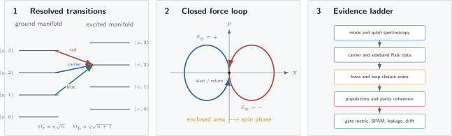
Carrier and first-sideband resonances address different pairs of $|g,n\rangle$ and $|e,n'\rangle$ states. A balanced bichromatic drive can turn those couplings into a spin-dependent force: the motional state follows opposite phase-space trajectories for different spin projections and returns after a closed loop. The enclosed area produces a spin phase, but a gate claim also requires spectroscopy, loop-closure tests, entanglement evidence, and a metric that separates gate error from state preparation and measurement.

Beyond the First-Order Picture

Higher sidebands

The $s$th motional sideband changes $n$ by $s$ and has a leading matrix element proportional to $\eta^{|s|}$. Higher sidebands are weak in a deep Lamb–Dicke regime but can be intentionally driven for state synthesis or can appear as leakage when the mode is hot.

Off-resonant terms

Driving the red sideband also drives the carrier off resonance by $\nu$ and other sidebands by integer multiples of $\nu$. A rough rectangular-pulse scale for an off-resonant carrier contribution is

$$\epsilon_{\mathrm{off}} \sim \left( \frac{\Omega}{\nu} \right)^2,$$

away from accidental cancellations. This is not a universal error formula: the exact probability depends on pulse duration, detuning, phase, AC Stark shifts, and all other levels and modes. It does show why increasing optical power does not indefinitely speed a spectrally selective sideband pulse.

AC Stark shifts

Off-resonant carrier, sideband, and auxiliary-level couplings shift the qubit resonance. A compensated pulse may use:

• a calibrated frequency offset;
• balanced red and blue components;
• pulse shaping;
• additional compensation light;
• a symmetric echo sequence.

The compensation must be validated over intensity and detuning drift. Canceling the mean shift does not automatically cancel its noise.

Direct Optical, Raman, and Microwave Control

Direct optical qubits

A narrow optical transition can directly couple $|g\rangle$ and $|e\rangle$. Its phase is inherited from the optical local oscillator at the ion. Direct sidebands use the single-beam wavevector projection and can be highly resolved, but gate and Ramsey coherence depend on optical phase stability and the excited-state lifetime.

Stimulated Raman transitions

Two optical fields can couple two long-lived states through one or more off-resonant excited states. In a simple three-level, large-detuning model,

$$\Omega_{\mathrm{eff}} \propto \frac{\Omega_1\Omega_2^*}{\Delta},$$

with convention-dependent factors and multilevel sums. The same elimination produces differential AC Stark shifts and spontaneous scattering. Increasing $|\Delta|$ suppresses excited-state population but requires more optical power for a fixed effective rate.

Raman control separates two design choices:

• the frequency difference addresses the qubit;
• the wavevector difference controls motional sensitivity.

Thus one can use nearly copropagating beams for motion-insensitive rotations and a larger $\Delta\mathbf k$ for sidebands and forces.

Microwave and magnetic-gradient control

Microwave wavelengths make the free-space Lamb–Dicke parameter extremely small. Near-field magnetic gradients can restore spin–motion coupling by making the field amplitude or phase vary across the ion wavepacket. These methods can reduce spontaneous optical scattering, but electrode currents, gradient calibration, motional-mode orientation, and microwave crosstalk become central.

Multi-Ion and Multimode Coupling

For ion $j$ and normal mode $m$, define

$$\eta_{jm} = \Delta\mathbf k \cdot \mathbf e_m\, b_{jm} \sqrt{ \frac{\hbar} {2m_j\omega_m} }.$$

Here $\mathbf e_m$ is a mode-polarization direction and $b_{jm}$ is the mass-weighted participation amplitude in the declared normalization. For mixed species or non-Cartesian modes, the normal-mode convention must be stated explicitly.

The interaction phase contains all modes:

$$\exp\!\left[ i \sum_m \eta_{jm} \left( a_me^{-i\omega_mt} + a_m^\dagger e^{i\omega_mt} \right) \right].$$

This expression gives several immediate lessons:

1. an ion can be nearly dark to a mode because $b_{jm}$ is small;
2. a laser can be dark to a mode because its wavevector is perpendicular to the polarization;
3. lower-frequency modes have larger zero-point extent and therefore larger $\eta_{jm}$, all else equal;
4. every occupied spectator mode contributes a Debye–Waller factor;
5. a multi-ion gate must close the phase-space displacement of every significantly coupled mode, not just the target mode.

Mode-frequency drift and avoided crossings can change both $\omega_m$ and $b_{jm}$. Recalibrating only one resonance may miss a changing mode participation pattern.

State Preparation and Ground-State Cooling

Internal preparation

Optical pumping prepares a chosen Zeeman or hyperfine state by repeated absorption and spontaneous emission. A complete preparation model includes polarization impurity, magnetic-field alignment, branching ratios, off-resonant excitation, metastable leakage, and repumping. A dark fluorescence result after pumping can represent successful preparation, population in an unintended dark level, or loss; independent checks are needed.

Motional preparation

In resolved-sideband cooling, the controlled step

$$|g,n\rangle \longrightarrow |e,n-1\rangle$$

is followed by dissipative repumping that returns the internal state while usually preserving $n-1$ in the Lamb–Dicke regime. Repetition drives population toward $|g,0\rangle$.

The control perspective emphasizes three requirements:

1. the red-sideband pulse must address the occupied range of $\sqrt n$-dependent Rabi frequencies;
2. repumping must remove internal entropy without adding too many motional quanta;
3. all modes needed by the subsequent operation must be cooled or shown to be harmless.

Continuous sideband cooling, pulsed sequences, Raman sideband cooling, EIT cooling, and sympathetic cooling solve different versions of this control problem. Their general dissipative and thermodynamic treatment belongs to Laser Cooling.

Verifying preparation

For a thermal mode under weak resolved-sideband probing,

$$\frac{I_{\mathrm r}}{I_{\mathrm b}} = \frac{\bar n}{\bar n+1}.$$

The platform-level assumptions behind this thermometer are discussed in Ion Traps. For coherent control, one should also inspect Rabi data, because different nonthermal distributions can share the same mean occupation or integrated sideband ratio.

Single-Qubit Control

Resonant rotations

A resonant carrier pulse realizes $R_\phi(\theta)$. Two orthogonal phase choices supply $X$- and $Y$-axis rotations. A frame update changes the phase assigned to subsequent drives and implements an idealized virtual $Z$ rotation without waiting for physical precession.

For a constant detuning error $\Delta$, the rotating-frame Hamiltonian is

$$H_{\mathrm{rot}} = \frac{\hbar}{2} \left( \Omega\sigma_\phi - \Delta\sigma_z \right).$$

The rotation axis tilts and the angular rate becomes

$$\Omega_R = \sqrt{\Omega^2+\Delta^2}.$$

Amplitude, phase, detuning, and timing errors therefore correspond to different geometric errors on the Bloch sphere and should be calibrated separately.

Composite and shaped pulses

Composite pulses can suppress selected systematic errors by arranging a sequence whose leading error terms cancel. Smooth envelopes can limit spectral leakage and transient response. Numerically optimized pulses can address mode crowding, crosstalk, or bandwidth constraints.

Robustness is never absolute. A pulse optimized against quasistatic amplitude error may be more sensitive to high-frequency phase noise or transfer-function distortion. Optimal Control and Dynamical Decoupling own the general control theory.

Motion as a Quantum Bus

The Coulomb interaction makes the secular normal modes collective. A field focused on ion $j$ can add a phonon amplitude to a shared mode, and a field on ion $k$ can respond to that same mode. Motion therefore mediates an interaction between internal states that do not directly couple at useful strength.

The bus analogy has limits:

• the bus contains several modes, not one ideal oscillator;
• heating and dephasing occur while the bus is used;
• the coupling is set by $\eta_{jm}$ and optical phase;
• residual spin–motion entanglement is coherent gate error, not merely a hot final state;
• a gate can be insensitive to the initial motional state only under declared approximations and closure conditions.

Cirac–Zoller Gate Principle

The original Cirac–Zoller proposal uses sideband pulses to map the state of a control ion onto a shared phonon, applies a phonon-conditioned operation to a target ion, and maps the phonon back. In schematic form,

$$\text{control spin} \longrightarrow \text{shared motion} \longrightarrow \text{target spin} \longrightarrow \text{motion reset}.$$

An auxiliary internal level and number-selective sideband dynamics provide the conditional phase. The construction made the physical role of a quantized bus explicit and motivated the first trapped-ion quantum logic experiments.

Its strict form requires near-ground-state motion and precise individual addressing. Modern gates more often use spin-dependent forces whose phase-space loop closes without populating a definite one-phonon bus state. The Cirac–Zoller protocol remains conceptually important because it exposes the sequence of mapping, conditional action, and unmapping.

Closed-Loop Spin-Dependent-Force Gates

Effective force Hamiltonian

A bichromatic field with components near the red and blue sidebands can be chosen at

$$\omega_{L,\pm} = \omega_0 \pm \left( \omega_m+\delta_g \right),$$

where $\delta_g$ is the symmetric detuning from one selected mode. After the internal and vibrational rotating-wave approximations, balanced phases give a spin-dependent force.

Write a convenient one-mode convention as

$$H_F(t) = i\hbar gS_\phi \left( a^\dagger e^{i\delta_gt} - a e^{-i\delta_gt} \right),$$

where:

• $S_\phi$ is a collective spin operator;
• $g$ is a calibrated force rate proportional to a sideband coupling;
• phases have been absorbed into $S_\phi$ and the oscillator coordinates.

For two equally driven ions, take

$$S_\phi = \frac{1}{2} \left( \sigma_\phi^{(1)} + \sigma_\phi^{(2)} \right).$$

Exact propagator in the effective model

Because $H_F$ is linear in $a$ and $a^\dagger$ and its commutator at two times is proportional to $S_\phi^2$, the Magnus expansion terminates after the second term. The propagator is

$$U(t) = D\!\left[ \alpha(t)S_\phi \right] \exp\!\left[ i\Phi(t)S_\phi^2 \right],$$

where

$$D(\zeta) = \exp\!\left( \zeta a^\dagger-\zeta^*a \right),$$

and

$$\alpha(t) = \frac{g}{i\delta_g} \left( e^{i\delta_gt}-1 \right).$$

The geometric phase is

$$\Phi(t) = \left( \frac{g}{\delta_g} \right)^2 \left[ \delta_gt-\sin(\delta_gt) \right].$$

The displacement $D[\alpha S_\phi]$ entangles spin and motion during the gate. The phase $\Phi$ equals the signed area enclosed by the phase-space trajectory, in the chosen normalization.

Loop closure and entanglement

At

$$t_g = \frac{2\pi}{|\delta_g|},$$

the displacement closes:

$$\alpha(t_g)=0.$$

The remaining ideal operation is

$$U_g = \exp\!\left( i\Phi_gS_\phi^2 \right), \qquad \Phi_g = 2\pi \left( \frac{g}{\delta_g} \right)^2.$$

For two ions,

$$S_\phi^2 = \frac{1}{2}I + \frac{1}{2} \sigma_\phi^{(1)} \sigma_\phi^{(2)}.$$

Apart from a global phase,

$$U_g \sim \exp\!\left[ i\frac{\Phi_g}{2} \sigma_\phi^{(1)} \sigma_\phi^{(2)} \right].$$

A maximally entangling operation has

$$|\Phi_g| = \frac{\pi}{2},$$

which in this convention corresponds to

$$\left| \frac{g}{\delta_g} \right| = \frac{1}{2}.$$

Different definitions of $S_\phi$, $\Omega$, or bichromatic amplitude move factors of two between $g$ and $\Phi_g$. A reported gate parameter set must state the Hamiltonian convention or provide a direct calibration.

Why thermal motion can cancel

If $\alpha(t_g)=0$, the ideal final propagator contains no oscillator operator. It therefore acts identically on every initial motional state in the effective model. This is the central robustness of Mølmer–Sørensen and related geometric-phase gates.

It does not mean cooling is unnecessary. The derivation still requires:

• Lamb–Dicke validity over the occupied distribution;
• negligible heating and mode-frequency drift during the loop;
• closure for every coupled mode;
• sufficiently uniform force over the wavepacket;
• controlled off-resonant carrier and spectator transitions.

The correct statement is that the gate need not resolve or populate one specific motional Fock state when the force loop closes.

Multimode Gate Design

With several modes, the effective propagator contains a spin-conditioned multimode displacement of the form

$$\exp\!\left\{ \sum_m \left[ \alpha_m(t)a_m^\dagger - \alpha_m^*(t)a_m \right] S_m \right\},$$

conditioned on collective spin operators. A spin-only gate requires

$$\alpha_m(t_g)=0$$

for every appreciably coupled mode $m$.

Single rectangular pulses generally close one selected mode exactly and leave small spectator loops. Strategies for multimode closure include:

• choosing detunings in a sparse part of the spectrum;
• amplitude or phase modulation;
• segmented pulses whose displacement vectors sum to zero;
• Walsh or other sign modulation;
• numerical optimization with measured mode frequencies and transfer functions;
• transporting ions into smaller interaction zones.

The pulse should be tested against out-of-sample mode-frequency shifts, heating, intensity imbalance, and calibration drift. A mathematically closed loop in a nominal model is not evidence that the laboratory loop closes.

Worked Scale Audit: Optical Sidebands

Consider an idealized $^{40}\mathrm{Ca}^+$ ion with a secular mode at

$$\frac{\nu}{2\pi} = 1.50\ \mathrm{MHz}.$$

For a direct $729\ \mathrm{nm}$ optical drive whose wavevector makes a $45^\circ$ angle with the mode,

$$k_{\mathrm{eff}} = \frac{2\pi}{729\ \mathrm{nm}} \cos45^\circ.$$

Using $m=39.9626\,u$ gives

$$x_0 = \sqrt{\frac{\hbar}{2m\nu}} = 9.18\ \mathrm{nm},$$

and

$$\eta = k_{\mathrm{eff}}x_0 = 0.05596.$$

Suppose the calibrated carrier rate is

$$\frac{\Omega}{2\pi} = 50.0\ \mathrm{kHz}.$$

The carrier $\pi$ time is

$$t_{\pi,\mathrm c} = \frac{\pi}{\Omega} = 10.0\ \mu\mathrm{s}.$$

For $n=1$, the leading red-sideband rate is

$$\frac{\Omega_{\mathrm r}(1)}{2\pi} \simeq \eta \frac{\Omega}{2\pi} = 2.80\ \mathrm{kHz},$$

so

$$t_{\pi,\mathrm r}(1) \simeq 179\ \mu\mathrm{s}.$$

The rough off-resonant-carrier scale is

$$\left( \frac{\Omega}{\nu} \right)^2 = 1.11\times10^{-3}.$$

This is only a scale: the actual error can oscillate with pulse duration and contains AC Stark shifts and other modes. For $\bar n=0.10$, the Lamb–Dicke parameter over the thermal extent is

$$\eta\sqrt{2\bar n+1} = 0.0613,$$

which supports a first-order treatment. At $\bar n=100$, the same quantity is $0.793$, so the geometry and trap frequency alone do not establish the Lamb–Dicke regime.

The example also shows a speed trade-off. Raising $\Omega$ shortens the sideband pulse but increases off-resonant coupling unless the mode frequency or pulse design changes.

Calibrating the Hamiltonian

Frequencies and phases

Measure and track:

• the qubit resonance and its magnetic- or light-shift dependence;
• all relevant motional frequencies and avoided crossings;
• red and blue sideband centers;
• optical, Raman, or microwave phase at the ion;
• phase transients from switches, modulators, and amplifiers.

A frequency counter at the source does not measure phase and amplitude after the complete optical or electrical transfer path.

Coupling strengths

Carrier Rabi data calibrate $\Omega$ only within a state and detuning model. Sideband Rabi data constrain $\eta_{jm}\Omega_j$ and the motional distribution. Independent geometry and mode calculations can separate $\eta_{jm}$ from $\Omega_j$, but their uncertainties must be propagated.

For a multimode gate, fit or bound:

• ion-dependent amplitudes $\Omega_j$;
• mode participations $b_{jm}$;
• bichromatic amplitude imbalance;
• sideband detunings;
• differential AC Stark shifts;
• spectator-mode couplings.

Motional reset

Loop closure can be tested by:

• adding an analysis displacement and reconstructing residual motion;
• varying the gate detuning or duration around the closure point;
• comparing spin coherence for different prepared motional occupations;
• inserting a second loop with reversed phase;
• measuring heating and mode drift over the gate duration.

High Bell-state contrast alone does not uniquely diagnose residual spin–motion entanglement, because other errors can reduce or mimic the same observable.

Evidence for an Entangling Gate

Bell-state evidence

For a target state

$$|\Psi\rangle = \frac{ |00\rangle + e^{i\varphi}|11\rangle }{\sqrt{2}},$$

the optimized fidelity is

$$F_{\mathrm{Bell}} = \frac{P_{00}+P_{11}}{2} + |\rho_{00,11}|.$$

A parity oscillation after a phase-scanned analysis pulse can measure a contrast

$$C=2|\rho_{00,11}|,$$

so under the declared analysis model,

$$F_{\mathrm{Bell}} = \frac{ P_{00}+P_{11}+C }{2}.$$

An entanglement witness is obtained when the fidelity exceeds the appropriate separable bound after uncertainties are included.

Why Bell fidelity is not gate fidelity

A Bell-state experiment combines:

• state preparation;
• one or more single-qubit rotations;
• the entangling pulse;
• idle evolution;
• analysis pulses;
• fluorescence measurement.

Its fidelity is a sequence-level state metric. It does not by itself identify the average fidelity of the entangling operation on arbitrary inputs.

Process tomography, gate-set tomography, interleaved randomized benchmarking, cycle benchmarking, and model-based error amplification answer different questions and make different assumptions. A mature report states:

1. the metric being estimated;
2. whether state-preparation and measurement errors are included or removed;
3. the statistical interval;
4. leakage treatment;
5. drift and temporal correlations;
6. which coherent errors benchmarking may randomize or hide.

Evidence ladder

Claim	Minimum direct evidence
resolved sideband control	spectrum plus coherent Rabi oscillations at the assigned resonance
ground-state preparation	calibrated red/blue asymmetry and a model check against Rabi data
spin-dependent force	force-dependent displacement or dephasing versus pulse phase and detuning
closed-loop gate	closure scan and bounded residual spin–motion correlation
entangled output	populations plus phase-sensitive coherence or another witness
calibrated gate	a gate metric with SPAM, leakage, drift, and uncertainty treatment

Error Budget

Residual displacement

If a mode does not close, the final displacement $\alpha_m$ leaves spin and motion entangled. For a thermal mode, spin coherence is suppressed by factors that scale with

$$|\alpha_m|^2(2\bar n_m+1).$$

The exact coefficient depends on the spin branches and observable. This scaling explains why a small detuning error can become more damaging at high motional occupation.

Motional heating and dephasing

Heating during the gate changes the enclosed trajectory stochastically and prevents perfect return. Mode-frequency noise changes both closure and geometric phase. A single pre-gate $\bar n$ measurement does not bound either effect; gate-duration heating and frequency-noise measurements are needed.

Spontaneous scattering

Raman or optical forces can scatter photons through off-resonant excited states. The error scale contains

$$p_{\mathrm{sc}} \sim \Gamma_{\mathrm{sc}}t_g,$$

but Raman, Rayleigh, leakage, and recoil channels have different effects. Detuning, polarization, fine structure, and laser power determine the trade-off.

Off-resonant excitation and light shifts

Fast gates increase carrier and spectator-sideband coupling. Unbalanced bichromatic fields produce differential Stark shifts and can rotate the spin while applying the force. Pulse shaping can suppress selected terms but may increase duration and heating exposure.

Lamb–Dicke breakdown

Higher powers of $\eta(a+a^\dagger)$ make the force depend on motional amplitude and invalidate exact phase-space closure. A useful diagnostic scale is

$$\eta^2(2\bar n+1).$$

The distribution tail can matter even when the mean passes a nominal test.

Qubit and control noise

Laser phase noise, microwave phase noise, magnetic-field fluctuations, intensity noise, timing jitter, addressing crosstalk, and waveform distortion act during carrier and entangling operations. Their impact depends on noise spectrum and control filter functions, not only RMS drift.

Preparation and measurement

SPAM error does not cease to matter because an experiment reports a background-subtracted contrast. State leakage, dark-state decay, camera crosstalk, threshold bias, and imperfect analysis rotations can all bias an inferred gate metric.

Common Mistakes

Using the wrong detuning sign

With $\delta=\omega_L-\omega_0$, the red sideband is at $\delta=-\nu$ and the blue sideband at $\delta=+\nu$. Other texts define detuning with the opposite sign. Copying a formula without its convention exchanges the labels.

Calling every narrow spectral line a sideband

RF micromotion sidebands, secular motional sidebands, Zeeman components, hyperfine transitions, and modulation artifacts can all flank a carrier. Their voltage, geometry, polarization, and frequency scaling distinguish them.

Treating the Lamb–Dicke parameter as species-only

$\eta$ depends on mass, mode frequency, mode participation, and effective wavevector direction. The regime also depends on the motional occupation.

Equating resolved sidebands with ground-state cooling

Resolution is a spectral condition. Ground-state preparation is a statement about populations and requires thermometry.

Omitting spectator modes

A bichromatic pulse near one mode still couples off resonantly to others. Every appreciable displacement must close or be bounded.

Saying a geometric gate never uses motion

Motion mediates the interaction and is generally entangled with spin during the pulse. The useful property is return to the initial motional state at loop closure.

Saying a Mølmer–Sørensen gate works at any temperature

Initial-state independence holds in the effective closed-loop model. Hot motion can violate the Lamb–Dicke approximation, amplify residual displacement, and increase sensitivity to anharmonicity.

Reporting Bell fidelity as average gate fidelity

The two metrics answer different questions. A Bell-state sequence can have high fidelity while the operation has input-dependent errors, and gate benchmarking can obscure leakage or drift if its model is incomplete.

Exercises

Exercise 1: Identify carrier and sidebands

Using the interaction

$$\begin{aligned} H_I(t) ={}& \frac{\hbar\Omega}{2} \sigma_+ \exp\!\left[ i\eta \left( ae^{-i\nu t} + a^\dagger e^{i\nu t} \right) \right] \\ &\times e^{-i(\delta t+\phi)} + \mathrm{h.c.}, \end{aligned}$$

expand to first order in $\eta$ and identify the resonant term for $\delta=0,-\nu,+\nu$.

Solution

The first-order expansion is

$$\begin{aligned} H_I(t) \simeq \frac{\hbar\Omega}{2}\sigma_+ \big[ 1 + i\eta ae^{-i\nu t} + i\eta a^\dagger e^{i\nu t} \big] e^{-i(\delta t+\phi)} + \mathrm{h.c.} \end{aligned}$$

At $\delta=0$, the constant term is stationary and gives

$$H_{\mathrm c} = \frac{\hbar\Omega}{2} \left( \sigma_+e^{-i\phi} + \sigma_-e^{i\phi} \right).$$

At $\delta=-\nu$, the factor $ae^{-i\nu t}$ multiplies $e^{+i\nu t}$ and is stationary:

$$H_{\mathrm r} = \frac{i\hbar\eta\Omega}{2} \left( \sigma_+a e^{-i\phi} - \sigma_-a^\dagger e^{i\phi} \right).$$

At $\delta=+\nu$, the factor $a^\dagger e^{i\nu t}$ multiplies $e^{-i\nu t}$ and is stationary:

$$H_{\mathrm b} = \frac{i\hbar\eta\Omega}{2} \left( \sigma_+a^\dagger e^{-i\phi} - \sigma_-a e^{i\phi} \right).$$

All other first-order terms rotate at $\nu$ or $2\nu$ and are neglected only when the vibrational rotating-wave approximation is valid.

Exercise 2: Number-dependent Rabi rates

Starting from the first-order sideband Hamiltonians, derive the red and blue Rabi rates from an initial state $|g,n\rangle$. Evaluate their ratio for $n=3$.

Solution

The ladder-operator matrix elements are

$$a|n\rangle = \sqrt n\,|n-1\rangle, \qquad a^\dagger|n\rangle = \sqrt{n+1}\,|n+1\rangle.$$

Therefore

$$\Omega_{\mathrm r}(n) = \eta\Omega\sqrt n, \qquad \Omega_{\mathrm b}(n) = \eta\Omega\sqrt{n+1}.$$

For $n=3$,

$$\frac{\Omega_{\mathrm b}(3)} {\Omega_{\mathrm r}(3)} = \sqrt{\frac{4}{3}} = \frac{2}{\sqrt3} \simeq 1.155.$$

The red rate vanishes at $n=0$, whereas the blue rate remains $\eta\Omega$ because it can create a phonon.

Exercise 3: Exact carrier correction

Use the exact carrier matrix element

$$\Omega_{n,n} = \Omega e^{-\eta^2/2}L_n(\eta^2)$$

to recover its expansion through order $\eta^2$. For $\eta=0.10$, compare the approximate carrier rates for $n=0$ and $n=10$.

Solution

For small $x$,

$$e^{-x/2} \simeq 1-\frac{x}{2}, \qquad L_n(x) \simeq 1-nx.$$

With $x=\eta^2$,

$$\frac{\Omega_{n,n}}{\Omega} \simeq \left( 1-\frac{\eta^2}{2} \right) \left( 1-n\eta^2 \right) \simeq 1-\eta^2 \left( n+\frac{1}{2} \right).$$

For $\eta=0.10$,

$$\frac{\Omega_{0,0}}{\Omega} \simeq 0.995,$$

whereas

$$\frac{\Omega_{10,10}}{\Omega} \simeq 0.895.$$

The difference is about $10\%$ of the bare rate. A broad number distribution therefore produces visible collapse and dephasing of carrier Rabi oscillations even in a closed system.

Exercise 4: Optical-sideband scale audit

Reproduce the worked $^{40}\mathrm{Ca}^+$ values for $x_0$, $\eta$, the $n=1$ red-sideband rate, and its $\pi$ time. How do $\eta$ and the sideband rate change if the optical wavevector is made perpendicular to the mode?

Solution

With

$$m=39.9626\,u, \qquad \nu=2\pi(1.50\ \mathrm{MHz}),$$

the zero-point length is

$$x_0 = \sqrt{\frac{\hbar}{2m\nu}} = 9.18\ \mathrm{nm}.$$

The projected wavevector is

$$k_{\mathrm{eff}} = \frac{2\pi}{729\ \mathrm{nm}} \cos45^\circ,$$

so

$$\eta=k_{\mathrm{eff}}x_0=0.05596.$$

For $\Omega/(2\pi)=50.0\ \mathrm{kHz}$,

$$\frac{\Omega_{\mathrm r}(1)}{2\pi} = \eta \frac{\Omega}{2\pi} = 2.80\ \mathrm{kHz}.$$

Thus

$$t_{\pi,\mathrm r}(1) = \frac{\pi}{\Omega_{\mathrm r}(1)} = \frac{1} {2(2.80\ \mathrm{kHz})} \simeq 179\ \mu\mathrm{s}.$$

If the wavevector is perpendicular to the mode, $k_{\mathrm{eff}}=0$ in the ideal geometry. Then $\eta=0$ and the motional sideband vanishes, while the internal carrier can remain. Small residual sidebands can diagnose angular misalignment, mode rotation, or another wavevector component.

Exercise 5: Sideband thermometry and model checking

A mode has measured weak-probe sideband ratio $I_{\mathrm r}/I_{\mathrm b}=0.20$. Infer $\bar n$ and the thermal ground-state probability. Explain why observing the same ratio at twice the probe power is not automatically a successful consistency check.

Solution

For the ideal thermal weak-probe relation,

$$R = \frac{\bar n}{\bar n+1}.$$

Hence

$$\bar n = \frac{R}{1-R} = \frac{0.20}{0.80} = 0.25.$$

For a thermal oscillator,

$$P_0 = \frac{1}{1+\bar n} = 0.80.$$

At larger probe power, saturation, power broadening, off-resonant carrier excitation, and probe-induced heating can change red and blue areas. If both areas are biased by similar factors, their ratio may remain $0.20$ despite a failed weak-probe model. A useful check also varies pulse duration, fits Rabi data, examines residuals, and tests for nonthermal populations.

Exercise 6: A mode-dark ion

Three equal ions have an ideal axial mode with normalized participation vector

$$\mathbf b = \frac{1}{\sqrt2} \left( 1,0,-1 \right).$$

All ions are illuminated with the same wavevector projection and optical Rabi frequency. Compare their Lamb–Dicke parameters and explain the control consequence.

Solution

For equal masses and a common beam geometry,

$$\eta_{jm} \propto b_{jm}.$$

Therefore

$$\eta_{1m} = \frac{\eta_0}{\sqrt2}, \qquad \eta_{2m}=0, \qquad \eta_{3m} = - \frac{\eta_0}{\sqrt2},$$

for an appropriate common scale $\eta_0$.

The middle ion is dark to this mode at first order, although its carrier can still be driven. The two outer ions couple with equal magnitude and opposite sign, which changes the phase of a spin-dependent force. Addressing the middle ion cannot directly add a phonon to this ideal mode; any observed coupling constrains symmetry breaking, mode mixing, beam gradients, or an incorrect mode assignment.

Exercise 7: Closed-loop entangling phase

For

$$H_F(t) = i\hbar gS_\phi \left( a^\dagger e^{i\delta_gt} - a e^{-i\delta_gt} \right),$$

show that the displacement closes at $t_g=2\pi/|\delta_g|$. If $g/(2\pi)=5.00\ \mathrm{kHz}$ and $\delta_g/(2\pi)=10.0\ \mathrm{kHz}$, find $t_g$ and $\Phi_g$. Is the two-ion gate maximally entangling in the convention of this page?

Solution

The displacement is

$$\alpha(t) = \frac{g}{i\delta_g} \left( e^{i\delta_gt}-1 \right).$$

At

$$t_g = \frac{2\pi}{|\delta_g|},$$

the exponential is unity, so $\alpha(t_g)=0$.

For $\delta_g/(2\pi)=10.0\ \mathrm{kHz}$,

$$t_g = \frac{1}{10.0\ \mathrm{kHz}} = 100\ \mu\mathrm{s}.$$

The geometric phase is

$$\Phi_g = 2\pi \left( \frac{g}{\delta_g} \right)^2 = 2\pi \left( \frac{1}{2} \right)^2 = \frac{\pi}{2}.$$

With $S_\phi=(\sigma_\phi^{(1)}+\sigma_\phi^{(2)})/2$, this gives the entangling part

$$\exp\!\left[ i\frac{\pi}{4} \sigma_\phi^{(1)} \sigma_\phi^{(2)} \right],$$

up to a global phase. It is maximally entangling.

Exercise 8: Design a gate-evidence package

An experiment produces a Bell-state fidelity of $0.985$ after one bichromatic pulse and claims a two-qubit gate fidelity of $0.985$. Identify what is missing and design a minimal set of additional measurements.

Solution

The Bell-state number is a sequence-level state fidelity, not automatically an average gate fidelity. It includes preparation, single-qubit rotations, the entangling pulse, idle evolution, analysis rotations, and measurement. It may also probe only one input state and one coherence.

A minimal additional package would include:

1. raw and corrected populations plus the phase-scanned parity data and fit residuals;
2. independent SPAM and single-qubit calibration, including leakage;
3. gate action on a set of inputs or a validated benchmarking protocol;
4. a loop-closure scan versus gate duration and bichromatic detuning;
5. mode occupations, heating rates, and relevant frequency drift;
6. tests versus bichromatic amplitude balance, optical phase, and spectator modes;
7. repeated or interleaved measurements to expose drift;
8. a statistical interval and an explicit definition of the reported gate metric.

Process tomography could reconstruct a candidate channel but is itself SPAM-sensitive. Interleaved randomized benchmarking can estimate an average error under assumptions about reference gates and temporal stationarity but can obscure leakage or coherent drift. Using more than one diagnostic is valuable because their failure modes differ.

References

1. D. Leibfried, R. Blatt, C. Monroe, and D. Wineland, “Quantum dynamics of single trapped ions,” Reviews of Modern Physics 75, 281–324 (2003), doi:10.1103/RevModPhys.75.281.
2. D. J. Wineland, C. Monroe, W. M. Itano, D. Leibfried, B. E. King, and D. M. Meekhof, “Experimental issues in coherent quantum-state manipulation of trapped atomic ions,” Journal of Research of the National Institute of Standards and Technology 103, 259–328 (1998), doi:10.6028/jres.103.019.
3. D. F. V. James, “Quantum dynamics of cold trapped ions with application to quantum computation,” Applied Physics B 66, 181–190 (1998), doi:10.1007/s003400050373.
4. J. I. Cirac and P. Zoller, “Quantum computations with cold trapped ions,” Physical Review Letters 74, 4091–4094 (1995), doi:10.1103/PhysRevLett.74.4091.
5. C. Monroe, D. M. Meekhof, B. E. King, W. M. Itano, and D. J. Wineland, “Demonstration of a fundamental quantum logic gate,” Physical Review Letters 75, 4714–4717 (1995), doi:10.1103/PhysRevLett.75.4714.
6. D. M. Meekhof, C. Monroe, B. E. King, W. M. Itano, and D. J. Wineland, “Generation of nonclassical motional states of a trapped atom,” Physical Review Letters 76, 1796–1799 (1996), doi:10.1103/PhysRevLett.76.1796.
7. F. Diedrich, J. C. Bergquist, W. M. Itano, and D. J. Wineland, “Laser cooling to the zero-point energy of motion,” Physical Review Letters 62, 403–406 (1989), doi:10.1103/PhysRevLett.62.403.
8. A. Sørensen and K. Mølmer, “Quantum computation with ions in thermal motion,” Physical Review Letters 82, 1971–1974 (1999), doi:10.1103/PhysRevLett.82.1971.
9. A. Sørensen and K. Mølmer, “Entanglement and quantum computation with ions in thermal motion,” Physical Review A 62, 022311 (2000), doi:10.1103/PhysRevA.62.022311.
10. C. A. Sackett et al., “Experimental entanglement of four particles,” Nature 404, 256–259 (2000), doi:10.1038/35005011.
11. D. Leibfried et al., “Experimental demonstration of a robust, high-fidelity geometric two ion-qubit phase gate,” Nature 422, 412–415 (2003), doi:10.1038/nature01492.
12. F. Schmidt-Kaler et al., “Realization of the Cirac–Zoller controlled-NOT quantum gate,” Nature 422, 408–411 (2003), doi:10.1038/nature01494.
13. C. F. Roos, “Ion trap quantum gates with amplitude-modulated laser beams,” New Journal of Physics 10, 013002 (2008), doi:10.1088/1367-2630/10/1/013002.
14. H. Häffner, C. F. Roos, and R. Blatt, “Quantum computing with trapped ions,” Physics Reports 469, 155–203 (2008), doi:10.1016/j.physrep.2008.09.003.
15. J. Benhelm, G. Kirchmair, C. F. Roos, and R. Blatt, “Towards fault-tolerant quantum computing with trapped ions,” Nature Physics 4, 463–466 (2008), doi:10.1038/nphys961.
16. C. J. Ballance, T. P. Harty, N. M. Linke, M. A. Sepiol, and D. M. Lucas, “High-fidelity quantum logic gates using trapped-ion hyperfine qubits,” Physical Review Letters 117, 060504 (2016), doi:10.1103/PhysRevLett.117.060504.
17. J. P. Gaebler et al., “High-fidelity universal gate set for $^9\mathrm{Be}^+$ ion qubits,” Physical Review Letters 117, 060505 (2016), doi:10.1103/PhysRevLett.117.060505.
18. C. D. Bruzewicz, J. Chiaverini, R. McConnell, and J. M. Sage, “Trapped-ion quantum computing: Progress and challenges,” Applied Physics Reviews 6, 021314 (2019), doi:10.1063/1.5088164.

Cross-Links

• Ion Traps develops the confinement and normal modes assumed throughout this page.
• Jaynes–Cummings Model gives the canonical exchange dynamics realized by a red motional sideband.
• Rabi Oscillations develops coherent two-level rotations before motional coupling is included.
• Bell States supplies the entanglement structure used in two-ion state validation.
• Trapped Ions follows the same platform through heating, dephasing, fluorescence, and quantum trajectories.
• Quantum Information Roadmap connects physical gate primitives to the broader formal and computational study path.