Cold Molecules

A cold-molecule platform controls both the center-of-mass motion of a molecule and a declared subset of its electronic, vibrational, rotational, hyperfine, and parity states. Low translational temperature alone is not enough. A sample can be cold in velocity while occupying many unresolved internal states, or it can be internally pure while remaining too hot to trap, collide in a single partial wave, or resolve motional sidebands.

Molecules are attractive quantum systems for the same reason they are difficult ones. Their internal structure supplies:

• microwave-frequency rotational transitions;
• vibrational and electronic transitions over a wide spectral range;
• closely spaced opposite-parity levels;
• large molecule-frame electric dipole moments;
• nuclear-spin and hyperfine degrees of freedom; and
• sensitivity to short-range chemistry and symmetry-violating interactions.

Turning those resources into a trustworthy experiment requires an end-to-end chain:

1. produce slow molecules or assemble them from cold atoms;
2. close unwanted radiative and collisional channels;
3. prepare a resolved internal and motional state;
4. trap the sample without uncontrolled differential shifts;
5. calibrate electric, magnetic, microwave, and optical couplings;
6. measure with a characterized confusion or loss model; and
7. validate the claimed effective Hamiltonian against independent observables.

This page develops that platform layer quantitatively.

Canonical Scope

Molecular Quantum Mechanics owns the laboratory-frame molecular Hamiltonian, Born–Oppenheimer separation, potential-energy surfaces, bonding, and the hierarchy of electronic and nuclear motion. Rotations of Molecules and Vibrations of Diatomics derive the corresponding spectra and approximations.

Laser Cooling owns the general momentum-transfer and scattering-force framework. STIRAP owns the three-state adiabatic-transfer derivation. Optical Dipole Traps and Optical Tweezers own the general conservative-trapping theory and single-site control workflow.

This page instead owns:

• molecular photon-cycle closure and its photon-budget audit;
• direct cooling versus assembly from ultracold atoms;
• state preparation, trapping, and molecule-specific readout;
• field-induced dipoles, dipolar interactions, and collisional loss;
• the platform requirements for precision measurement and quantum simulation; and
• an evidence ladder for molecular control claims.

It does not duplicate full molecular-structure derivations, reaction scattering theory, or a catalog of individual molecular species.

What “Cold” Must Specify

Several temperatures and several purities

For atoms with a simple ground manifold, one temperature can sometimes summarize a useful equilibrium state. For molecules, at least four distributions may matter:

$$\rho \sim \rho_{\mathrm{trans}} \otimes \rho_{\mathrm{rot}} \otimes \rho_{\mathrm{vib}} \otimes \rho_{\mathrm{hf}},$$

when correlations among those sectors can be neglected. The labels

$$T_{\mathrm{trans}}, \qquad T_{\mathrm{rot}}, \qquad T_{\mathrm{vib}},$$

need not agree. Hyperfine populations may not be thermal at all.

An assembled molecule can inherit nanokelvin center-of-mass motion from its constituent atoms and be transferred into one rovibrational level, yet still occupy several unresolved nuclear-spin states. A buffer-gas beam can have kelvin-scale rotational cooling and a narrow forward velocity distribution without being in the ultracold collision regime. A directly laser-cooled sample can be translationally cold but distributed among Zeeman sublevels that must be remixed during cycling.

Therefore a useful sample description reports:

• translational temperature or motional-state distribution;
• density or site occupation;
• electronic, vibrational, rotational, and hyperfine populations;
• trap geometry and dimensionality;
• electric and magnetic bias fields;
• lifetime and loss law; and
• the method used to infer each quantity.

Operational regimes

There is no universal temperature boundary that makes every molecule “cold” or “ultracold.” The physically relevant comparisons are operational:

$$k_B T \quad\text{versus}\quad \hbar\omega_{\mathrm{trap}}, \ B_{\mathrm{rot}}, \ E_{\mathrm{hf}}, \ E_{\mathrm{collision}}, \ \hbar\Gamma,$$

where $B_{\mathrm{rot}}$ here denotes a rotational energy scale rather than a magnetic field.

Examples include:

• resolved motion: $k_B T\lesssim\hbar\omega_{\mathrm{trap}}$ or direct evidence of a large ground-state occupation;
• few-partial-wave collisions: the collision energy is below relevant centrifugal barriers;
• resolved internal control: drive linewidths and inhomogeneous shifts are smaller than the selected level spacings;
• quantum degeneracy: phase-space density and statistics, not temperature alone, meet the appropriate many-body criterion.

Calling a sample ultracold should be followed by the operational fact that the low temperature enables.

Why Molecules Are Harder Than Atoms

A useful platform Hamiltonian

After selecting a tractable internal manifold, a molecular apparatus is often organized as

$$H = \frac{\mathbf p^2}{2M} +H_{\mathrm{int}} +H_{\mathrm{trap}}(\mathbf r) +H_{\mathrm{field}} +H_{\mathrm{drive}} +\sum_{i<j}V_{ij}.$$

The terms carry coupled responsibilities:

• $H_{\mathrm{int}}$ contains rotational, vibrational, spin-rotation, hyperfine, parity-doublet, and Zeeman structure;
• $H_{\mathrm{trap}}$ can depend on the internal state through scalar, vector, and tensor polarizabilities;
• $H_{\mathrm{field}}$ mixes parity and angular-momentum states;
• $H_{\mathrm{drive}}$ addresses optical, microwave, or radio-frequency transitions; and
• $V_{ij}$ may include anisotropic dipolar coupling and short-range loss.

An effective two-level or spin model follows only after unwanted levels, motion, micromotion, photon scattering, and loss are bounded on the experimental timescale.

Radiative branching

An electronically excited atom often decays predominantly to one ground manifold. A molecule can decay into many vibrational and rotational levels. Every unaddressed branch is a path to a state dark to the cooling light.

The problem is multiplicative. A leak probability of only $10^{-4}$ per photon is large if a slowing stage needs $10^4$ photons.

Angular momentum and dark states

Rotational, spin-rotation, hyperfine, Zeeman, and parity labels produce many sublevels. Polarization selection rules can pump population into coherent or incoherent dark states even when vibrational branching is favorable. Magnetic remixing, polarization switching, radio-frequency modulation, or multiple optical frequencies may be part of the cooling mechanism rather than optional refinements.

State-dependent trapping

Molecular polarizability is generally anisotropic. Trap depth and ac Stark shift can depend on rotational projection, polarization, and field angle. The trapping light can therefore dephase a rotational superposition or move a two-photon resonance while still confining the molecule.

Short-range loss

Two molecules that reach short range may react chemically, change internal state, or form a long-lived collision complex that is subsequently lost. Even nominally nonreactive species can exhibit substantial loss. A large electric dipole moment does not guarantee a long-lived gas; it strengthens both useful long-range coupling and the need to control close encounters.

A molecule-frame dipole is not a laboratory dipole

A heteronuclear molecule can have a permanent body-fixed electric dipole moment $d$, while a field-free parity eigenstate has

$$\langle\mathbf d\rangle_{\mathrm{lab}} = 0.$$

A static electric field or microwave dressing must mix suitable opposite-parity rotational states to produce an oriented or induced laboratory-frame dipole. The relevant interaction is set by that dressed matrix element, not by the maximum body-fixed value quoted for the species.

Rotational and Vibrational Complexity

The usual hierarchy and its limits

For a stable electronic state of a small molecule, one often finds

$$\Delta E_{\mathrm{electronic}} \gg \Delta E_{\mathrm{vibrational}} \gg \Delta E_{\mathrm{rotational}} \gtrsim \Delta E_{\mathrm{hf}}.$$

This hierarchy is a guide, not a universal theorem. Spin-orbit coupling, parity doubling, near-degenerate vibrational modes, and accidental level crossings can reorder the smaller scales.

In a simple diatomic approximation,

$$E(v,N) \approx G(v) +B_vN(N+1) -D_v[N(N+1)]^2 +E_{\mathrm{fine/hf}},$$

where $v$ is vibrational and $N$ is rotational angular momentum excluding spin. The structural meaning of $G(v)$, $B_v$, and $D_v$ belongs to the canonical molecular pages. Here the operational point is that a cooling or control laser must respect all populated branches of this level structure.

Franck–Condon factors are necessary, not sufficient

For an electronic transition between vibrational states, the Franck–Condon factor is

$$q_{v'v} = \left| \langle \chi_{v'}^{(e)} | \chi_v^{(g)} \rangle \right|^2.$$

A nearly diagonal matrix, with $q_{00}$ close to unity, makes a short repump scheme possible. The actual spontaneous-emission branching fraction also contains transition-frequency and rotational line-strength factors:

$$b_{a\to f} = \frac{ \omega_{af}^3 q_{v'v} S_{af} }{ \displaystyle \sum_{f'} \omega_{af'}^3 q_{v'v'} S_{af'} }.$$

Here $S_{af}$ includes the relevant rotational, spin, hyperfine, and polarization matrix elements after unresolved components are summed consistently. A large $q_{00}$ does not by itself close rotation, parity, hyperfine structure, or decay through perturbing electronic states.

Closure is an engineering statement

A usable cycling scheme specifies:

1. the driven electronic branch and parity;
2. the vibrational levels addressed by repump lasers;
3. the rotational closure argument;
4. every resolved hyperfine or spin-rotation component;
5. the mechanism that destabilizes dark states;
6. the measured photon-scattering rate; and
7. the residual probability of leaving the addressed manifold.

Selection rules identify exact zeros in an ideal Hamiltonian. Cycle closure requires measured bounds after field mixing, off-resonant excitation, laser-spectrum impurities, and weak electronic-state mixing are included.

Direct Laser Cooling

Photon-cycle survival

Let $\epsilon$ be the total probability per spontaneous-emission event of entering an unaddressed state. If the leak is independent from cycle to cycle, the probability of remaining in the optical cycle after $N_\gamma$ photons is

$$P_{\mathrm{cyc}} = (1-\epsilon)^{N_\gamma} \approx \exp(-N_\gamma\epsilon),$$

where the exponential form requires $\epsilon\ll1$.

For a target survival $P_\star$,

$$\epsilon \lesssim -\frac{\ln P_\star}{N_\gamma}.$$

This relation is more informative than saying that a transition is “highly diagonal.” The acceptable leak depends on whether the experiment needs ten photons for detection, hundreds for cooling, or ten thousand for beam slowing.

Momentum budget

Absorption from a directed laser transfers momentum $\hbar k$. Spontaneous emission has zero mean momentum in an isotropic cycle but adds diffusion. Ignoring projection factors and transverse heating, changing the molecular speed by $\Delta v$ requires approximately

$$N_\gamma \approx \frac{M\Delta v}{\hbar k} = \frac{M\lambda\Delta v}{h}.$$

The single-photon recoil velocity is

$$v_r = \frac{\hbar k}{M} = \frac{h}{M\lambda}.$$

For an ideal saturated two-level transition, the largest scattering rate is of order $\Gamma/2$. A molecule generally has several ground sublevels and finite power distributed among sidebands and repumps, so the observed rate can be substantially smaller. Slowing distance must use the measured scattering force rather than the two-level upper bound.

Worked audit: a CaF-scale slowing stage

Take a molecule of mass

$$M = 59\,u = 9.80\times10^{-26}\,\mathrm{kg},$$

cycled at

$$\lambda = 606\,\mathrm{nm}.$$

Its recoil velocity is

$$\begin{aligned} v_r &= \frac{h}{M\lambda} \\ &= 1.12\times10^{-2}\,\mathrm{m\,s^{-1}}. \end{aligned}$$

Removing $\Delta v=100\,\mathrm{m\,s^{-1}}$ therefore takes

$$\begin{aligned} N_\gamma &\approx \frac{\Delta v}{v_r} \\ &= 8.96\times10^3. \end{aligned}$$

Requiring 90% of the molecules to remain in the addressed manifold gives

$$\begin{aligned} \epsilon &\lesssim -\frac{\ln(0.90)}{8.96\times10^3} \\ &= 1.18\times10^{-5} \end{aligned}$$

per scattered photon. That is the unaddressed total after all repumps and angular branches are counted. It is not merely $1-q_{00}$.

Rotational closure

Electric-dipole spontaneous emission obeys angular-momentum and parity selection rules. In laser-coolable diatomics, one commonly selects a branch whose excited angular momentum and parity prevent decay into higher rotational levels that would otherwise require many rotational repumps. A frequent design starts from an $N=1$ ground rotational manifold and an excited $J'=1/2$ manifold.

The exact closure argument is species and coupling-case dependent. It must use:

• the correct angular momentum excluding and including electron spin;
• excited- and ground-state parity;
• hyperfine resolution;
• magnetic-field-induced mixing; and
• weak admixture of nearby electronic states.

“$\Delta N=\pm1$” by itself is not a complete molecular cycling proof.

Dark-state destabilization

Many molecular cycling transitions are type-II systems, in which the excited manifold does not have more magnetic sublevels than the ground manifold. Fixed laser polarization can then create dark superpositions. Remedies include:

• rapidly switching polarization;
• switching the magnetic-field gradient synchronously;
• applying a remixing magnetic field;
• adding radio-frequency or microwave couplings; and
• driving all relevant hyperfine sidebands.

These methods change the steady-state force and sometimes its sign. A molecular magneto-optical trap is therefore characterized by measured restoring force, damping, capture velocity, scattering rate, cloud size, temperature, and lifetime, not merely by the presence of six beams and a quadrupole field.

From a beam to a trapped sample

A typical direct-cooling pipeline is:

1. create a cryogenic buffer-gas or slowed molecular beam;
2. transverse-cool and collimate it;
3. apply radiation-pressure or frequency-chirped slowing;
4. capture it in a molecular magneto-optical trap;
5. use sub-Doppler molasses where available;
6. load a magnetic, optical dipole, lattice, or tweezer trap; and
7. cool and pump into a selected internal and motional state.

Each handoff has an efficiency and a possible state-selection bias. Reporting only the final molecule number hides whether loss arose from photon-cycle leakage, phase-space mismatch, internal-state pumping, or trap loading.

Association from Ultracold Atoms

Pair preparation

The association route starts with two laser-coolable atomic species, or two internal states of one species, already cold and trapped. Molecule formation requires atom pairs to overlap in the same collision or motional channel. The pair-conversion probability therefore depends on:

• density and phase-space density in a bulk gas;
• double occupation in an optical lattice;
• relative motional ground-state occupation in a tweezer pair;
• spin preparation;
• magnetic-field stability; and
• the width and character of the chosen resonance.

Cooling the atoms first transfers much of the difficult entropy-removal problem to mature atomic techniques. It does not guarantee unit molecule filling.

Magnetoassociation

Near a magnetic Feshbach resonance, an open-channel atom pair is coupled to a closed-channel molecular state. Sweeping the magnetic field across the avoided crossing can convert an atom pair into a weakly bound Feshbach molecule.

The resulting molecule is large and weakly bound. It usually does not yet have the chemical stability, body-frame dipole, or rovibrational purity wanted for a platform. Its value is as a coherent bridge whose motional distribution remains inherited from the atoms.

Magnetoassociation efficiency should be reported conditional on verified atom-pair occupancy. Otherwise empty sites, singly occupied sites, and failed association are conflated.

Coherent transfer to a selected state

Let $|f\rangle$ be the Feshbach molecule, $|e\rangle$ an electronically excited bridge state, and $|g\rangle$ a deeply bound target state. Pump and Stokes couplings $\Omega_P$ and $\Omega_S$ form the instantaneous dark state

$$|D(t)\rangle = \cos\theta(t)|f\rangle - e^{i\phi(t)} \sin\theta(t)|g\rangle,$$

with

$$\tan\theta(t) = \frac{\Omega_P(t)}{\Omega_S(t)}.$$

Applying the Stokes field before the pump field rotates the dark state from $|f\rangle$ to $|g\rangle$ while ideally suppressing population of $|e\rangle$. Full adiabaticity, detuning, phase-noise, and dissipation conditions are developed on the STIRAP page.

For molecular assembly, the additional practical requirements are:

• sufficient transition dipole on both legs despite very different internuclear separations;
• an excited level with favorable singlet–triplet or other state mixing;
• two-photon linewidth narrower than the target resonance;
• calibrated differential Stark and Zeeman shifts;
• stable optical phase during the pulse pair;
• negligible motional excitation from photon recoil and trap change; and
• a reverse-transfer pathway for detection.

Low intermediate-state population is not evidence of perfect transfer. Population can remain in $|f\rangle$, enter other ground states, or be lost without producing obvious fluorescence.

End-to-end assembly efficiency

For a site-resolved experiment, a useful factorization is

$$P_{\mathrm{mol}} = P_{\mathrm{pair}} P_{\mathrm{assoc}} P_{\mathrm{ST}} P_{\mathrm{surv}},$$

where:

• $P_{\mathrm{pair}}$ is the probability of preparing the required atom pair;
• $P_{\mathrm{assoc}}$ is magnetoassociation efficiency conditioned on that pair;
• $P_{\mathrm{ST}}$ is transfer efficiency into the selected molecular state; and
• $P_{\mathrm{surv}}$ covers trapping and hold-time survival.

Round-trip STIRAP measures approximately $P_{\mathrm{ST}}^2$ only if forward and reverse transfer have equal efficiency and loss in the target state is separately bounded. Taking the square root without those checks can misestimate one-way fidelity.

Direct cooling and assembly are complementary

Criterion	Direct laser cooling	Assembly from ultracold atoms
Initial source	Molecular beam or pre-cooled molecules	Laser-cooled atoms
Main structural requirement	Quasi-closed optical cycle	Suitable atom pair, resonance, and transfer path
Translational entropy removal	Molecular photon scattering and trapping	Mostly completed in the atoms
Species reach	Includes radicals and some polyatomics	Strongest for atom pairs that can both be cooled
Internal-state endpoint	Requires pumping and repumping	Can target one rovibrational state coherently
Typical bottleneck	Branching, dark states, capture	Pair filling, association, coherent transfer
Natural readout	Fluorescence or state-selective loss	Reverse transfer, dissociation, atom imaging

Neither route is intrinsically more “quantum.” The appropriate comparison uses final state purity, phase-space density, number or filling, lifetime, control fidelity, and measurement performance.

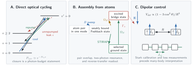
Three complementary layers of molecular control. A: direct cooling requires the unrepumped branching probability $\epsilon$ to be small on the full photon budget $N_\gamma$. B: atom-pair assembly separates magnetoassociation from coherent transfer and its lossy bridge state. C: a body-frame dipole becomes a calibrated laboratory interaction only after field dressing; loss and Stark-shift measurements are part of the Hamiltonian validation.

Trapping, State Preparation, and Readout

Conservative traps

Cold molecules can be confined in:

• magnetic traps, for low-field- or high-field-seeking magnetic states allowed by the geometry;
• electrostatic or alternating-gradient traps for suitable Stark states;
• optical dipole traps and optical lattices;
• optical tweezers for single-molecule control; and
• microwave-dressed traps in specialized regimes.

For an optical field, a selected state $|a\rangle$ experiences an ac Stark shift schematically of the form

$$U_a(\mathbf r) = -\frac{1}{4} \mathbf E_0^\ast(\mathbf r) \cdot \boldsymbol{\alpha}_a(\omega_L) \cdot \mathbf E_0(\mathbf r).$$

The tensor polarizability $\boldsymbol{\alpha}_a$ can mix rotational sublevels and create angle-dependent differential shifts. A trap wavelength or polarization that is benign for one transition need not be magic for another.

Trap characterization should include:

• depth and frequencies for each relevant internal state;
• differential ac Stark shift over the occupied spatial distribution;
• photon-scattering rate;
• parametric and technical heating;
• polarization purity and pointing stability; and
• lifetime with one molecule and with multiple molecules present.

Internal-state preparation

A state label should include every resolved quantum number needed to predict control and collisions. Depending on species and fields, a practical label may be

$$|\alpha;\,v,N,m_N;\,I,m_I;\,\mathcal P\rangle,$$

where $\alpha$ summarizes electronic structure and $\mathcal P$ denotes parity where it remains useful. In intermediate fields, such labels may be only adiabatic correlates; eigenstate composition should then be obtained from a diagonalized effective Hamiltonian.

Preparation tools include:

• optical pumping with vibrational and rotational repumps;
• microwave transfer among rotational and hyperfine states;
• radio-frequency transfer among Zeeman or nuclear-spin states;
• STIRAP or Raman transfer;
• adiabatic electric- or magnetic-field ramps; and
• state-selective removal of unwanted populations.

Preparation fidelity is measured by applying at least one independent analysis basis or transfer path. A single depletion pulse cannot distinguish perfect preparation from poor detection unless its own efficiency is known.

Readout modalities

Different production routes naturally support different detectors:

• cycling fluorescence: powerful for laser-coolable species, but photon collection and cycling survival must be calibrated;
• reverse association: transfer the molecule back to a Feshbach state, dissociate it, and image the atoms;
• state-selective depletion: remove one internal state and compare surviving populations;
• resonance-enhanced ionization: sensitive and state selective but destructive;
• absorption or fluorescence imaging: useful for ensembles when optical depth and branching are controlled; and
• loss detection in tweezers: site resolved, but intrinsically ambiguous unless molecular loss is distinguished from state transfer.

For a binary molecular-state measurement, write

$$\begin{pmatrix} q_{\mathrm{M}} \\ q_{\mathrm{not\,M}} \end{pmatrix} = \begin{pmatrix} 1-\epsilon_{\mathrm{fn}} & \epsilon_{\mathrm{fp}} \\ \epsilon_{\mathrm{fn}} & 1-\epsilon_{\mathrm{fp}} \end{pmatrix} \begin{pmatrix} p_{\mathrm{M}} \\ p_{\mathrm{not\,M}} \end{pmatrix}.$$

Here $\epsilon_{\mathrm{fn}}$ is the probability that an actual target molecule is reported absent, and $\epsilon_{\mathrm{fp}}$ is the probability that another condition is reported as the target. Inverting this matrix is useful only when its entries and uncertainties are independently measured and the matrix is well conditioned.

Electric-Field Control

Rigid-rotor polarization

For a linear rigid rotor with body-frame dipole magnitude $d$,

$$H_{\mathrm{rot+Stark}} = B_{\mathrm{rot}}\mathbf N^2 -d\mathcal E\cos\theta.$$

At zero field, parity makes the laboratory expectation of $d_z$ vanish. For the $N=0$ ground state, the leading coupling is to $N=1,m_N=0$, with matrix element

$$\langle 1,0|\cos\theta|0,0\rangle = \frac{1}{\sqrt3}.$$

When $d\mathcal E\ll B_{\mathrm{rot}}$, second-order perturbation theory gives

$$\Delta E_{00} \approx -\frac{d^2\mathcal E^2}{6B_{\mathrm{rot}}},$$

and the induced dipole is

$$d_{\mathrm{ind}} = -\frac{\partial\Delta E_{00}}{\partial\mathcal E} \approx \frac{d^2\mathcal E}{3B_{\mathrm{rot}}}.$$

This linear low-field result eventually saturates toward the body-frame scale as many rotational states mix. The exact Stark curve should be obtained by diagonalizing enough rotational levels and then checked spectroscopically.

Opposite-parity doublets

Some molecules possess a much smaller opposite-parity splitting $\delta$. In a two-state model,

$$H_{\mathcal P} = \begin{pmatrix} -\delta/2 & -d_{+-}\mathcal E \\ -d_{+-}\mathcal E & \delta/2 \end{pmatrix}.$$

The lower eigenenergy is

$$E_- = -\sqrt{ \left(\frac{\delta}{2}\right)^2 +d_{+-}^2\mathcal E^2 },$$

so

$$d_{\mathrm{ind}} = -\frac{\partial E_-}{\partial\mathcal E} = \frac{ d_{+-}^2\mathcal E }{ \sqrt{ (\delta/2)^2+d_{+-}^2\mathcal E^2 } }.$$

A small $\delta$ permits strong polarization at modest field. It also makes the state sensitive to stray electric fields and field gradients.

Field calibration

Electrode voltage is not the same as electric field at the molecules. Calibrate $\mathcal E$ by fitting measured Stark shifts to an internal-state Hamiltonian that includes:

• electrode geometry and voltage offsets;
• tensor Stark coupling;
• hyperfine and Zeeman terms;
• nearby avoided crossings;
• spatial gradients over the cloud or array; and
• microwave or optical dressing used during the measurement.

Reversing the applied voltage separates even and odd responses only after static offsets and imperfect reversal are included.

Dipolar Interactions

Pair interaction

Two laboratory-frame electric dipoles separated by $\mathbf R=R\hat{\mathbf R}$ interact as

$$V_{dd}(\mathbf R) = \frac{1}{4\pi\epsilon_0R^3} \left[ \mathbf d_1\cdot\mathbf d_2 -3 (\mathbf d_1\cdot\hat{\mathbf R}) (\mathbf d_2\cdot\hat{\mathbf R}) \right].$$

For parallel dipoles aligned by a field,

$$V_{dd} = \frac{ d_{\mathrm{ind}}^2 }{ 4\pi\epsilon_0R^3 } \left( 1-3\cos^2\theta \right),$$

where $\theta$ is the angle between the field and the intermolecular axis. The interaction is repulsive side by side, attractive head to tail, and vanishes at the magic angle

$$\cos^2\theta_m = \frac13.$$

This point-dipole form applies when $R$ is large compared with molecular size and the interaction does not strongly mix states omitted from the chosen manifold.

A one-Debye interaction audit

For

$$d_{\mathrm{ind}} = 1\,\mathrm D = 3.33564\times10^{-30}\,\mathrm{C\,m}$$

and $R=1\,\mu\mathrm m$, the base frequency scale is

$$\begin{aligned} \frac{1}{h} \frac{d_{\mathrm{ind}}^2}{4\pi\epsilon_0R^3} &= 151\,\mathrm{Hz}. \end{aligned}$$

Thus the side-by-side shift is $+151\,\mathrm{Hz}$ and the head-to-tail shift is $-302\,\mathrm{Hz}$. At $R=0.5\,\mu\mathrm m$, the base scale increases by $2^3=8$ to about $1.21\,\mathrm{kHz}$.

The sixth-power sensitivity of blockade radii does not appear here; direct dipolar coupling scales as $R^{-3}$. Position uncertainty and angular misalignment should therefore be propagated through both $R^{-3}$ and $1-3\cos^2\theta$.

Rotational spin exchange

Choose two rotational states $|\downarrow\rangle$ and $|\uparrow\rangle$. Dipole matrix elements can generate resonant exchange even when each field-free state has zero static dipole. In a pinned array, projection into the two-state manifold often yields

$$H_{\mathrm{spin}} = \sum_{i<j} \left[ \frac{J_{ij}^{\perp}}{2} \left( S_i^+S_j^- +S_i^-S_j^+ \right) +J_{ij}^zS_i^zS_j^z \right] +\sum_i h_iS_i^z.$$

The couplings inherit the spatial kernel

$$J_{ij} \propto \frac{ 1-3\cos^2\theta_{ij} }{ R_{ij}^3 }.$$

The coefficients depend on static and transition dipole matrix elements, microwave dressing, and the selected hyperfine states. Quoting only the body-frame dipole does not determine $J_{ij}^{\perp}$ or $J_{ij}^z$.

A credible spin-model realization verifies:

• single-molecule transition frequencies and Rabi couplings;
• differential Stark shifts across the array;
• field angle and polarization;
• pair or dilute-array exchange dynamics;
• occupancy and spatial correlations;
• loss and decoherence; and
• sensitivity to interactions outside the truncated manifold.

Collision and loss rates

For two-body loss in a homogeneous sample,

$$\frac{dn}{dt} = -\beta n^2,$$

so

$$n(t) = \frac{n_0}{1+\beta n_0t}.$$

The initial two-body loss timescale is

$$\tau_2 = \frac{1}{\beta n_0}.$$

At

$$\beta = 10^{-10}\,\mathrm{cm^3\,s^{-1}}, \qquad n_0 = 10^{11}\,\mathrm{cm^{-3}},$$

one obtains $\tau_2=0.10\,\mathrm s$. Reducing $\beta$ by two orders of magnitude increases this initial timescale to $10\,\mathrm s$, provided one-body loss and heating remain negligible.

For evaporative or rethermalizing collisions, the useful comparison is

$$\gamma_{\mathrm{el/loss}} = \frac{K_{\mathrm{el}}}{K_{\mathrm{loss}}},$$

not the elastic rate alone. A large ratio is needed for many elastic collisions before loss.

Suppressing short-range encounters

Strategies include:

• pinning molecules in a deep optical lattice or separated tweezers;
• confining fermionic molecules to exploit threshold and Pauli suppression;
• choosing field geometry that creates repulsive side-by-side interactions;
• microwave or static-field shielding;
• preparing nonreactive chemical species and selected spin states; and
• lowering density when coherence matters more than collision rate.

Shielding is a dressed multichannel scattering problem. Its evidence should include both reduced loss and the elastic interaction or thermalization that remains. A longer lifetime alone could result from lower density, poorer state preparation, or reduced overlap.

Precision Measurement

Why molecules can be sensitive

Molecular spectra contain ratios of electronic, vibrational, rotational, and hyperfine scales. Some states have strong internal effective electric fields or closely spaced opposite-parity partners. These properties can enhance sensitivity to:

• permanent electric dipole moments and other symmetry-violating interactions;
• variation of dimensionless constants;
• nuclear moments and nuclear-spin-dependent effects;
• parity violation; and
• isotope-dependent short-range physics.

Enhancement is not accuracy. Closely spaced states are also sensitive to stray fields, geometric phases, leakage, tensor light shifts, and imperfect reversal.

Phase accumulation and sensitivity coefficients

For a Ramsey-like interrogation of duration $T$, a small frequency shift $\delta\omega$ gives

$$\delta\phi = \delta\omega T.$$

If a transition frequency $\nu$ depends on a dimensionless parameter $X$, a sensitivity coefficient is

$$K_X = \frac{\partial\ln\nu}{\partial\ln X},$$

so

$$\frac{\delta\nu}{\nu} = K_X \frac{\delta X}{X}$$

to first order. The Precision Spectroscopy page owns frequency estimation and uncertainty budgets. The platform task here is to make state preparation, interrogation time, reversals, and readout sufficiently controlled that the inferred line shift has the claimed interpretation.

Reversal channels

A symmetry-sensitive experiment commonly changes signs of electric field, magnetic field, molecular orientation, polarization, propagation direction, or internal-state label. Let $s_k=\pm1$ denote reversal switches. A measured phase can be expanded as

$$\phi(\mathbf s) = \sum_A c_A \prod_{k\in A}s_k.$$

The desired signal occupies one parity channel in this switch space. Leakage into that channel occurs when reversals are correlated with field magnitude, detuning, contrast, trajectory, or readout. Randomization, blinding, auxiliary channels, and explicit covariance analysis are therefore part of molecular control rather than post-processing decoration.

Quantum Simulation

What molecules add

Rotational states offer stable microwave-addressed basis states, while electric dipole matrix elements provide anisotropic interactions extending beyond nearest neighbors. Field and microwave dressing can tune:

• exchange versus Ising-like coupling;
• interaction sign and angular dependence;
• internal-state-dependent hopping;
• spin-motion coupling; and
• collision pathways.

Optical lattices suppress motion and close encounters. Tweezers provide geometry and single-site readout. Bulk gases permit mobile dipolar matter and controlled chemistry but place greater demands on collisional stability.

Validation before extrapolation

A many-body observation should be tied to independently measured microscopic parameters. A useful progression is:

1. fit single-molecule spectroscopy and Stark shifts;
2. measure preparation and readout matrices;
3. calibrate two-molecule exchange or collisional rates;
4. validate a small system where exact modeling is possible;
5. vary density, spacing, angle, and dressing parameters;
6. test omitted couplings and loss channels; and
7. only then interpret large-system dynamics with an effective model.

Agreement at one time or one observable does not uniquely validate a Hamiltonian. Spatially resolved correlations, reversal of interaction sign, and parameter-scaling tests are stronger evidence.

Platform Error and Evidence Ledger

Layer	Quantity to calibrate	Independent observable	Common confounder
Source	Flux and velocity distribution	Time of flight	State-dependent detection
Optical cycle	Branching and scattering rate	Repump removal, fluorescence versus time	Dark-state pumping
Capture	Restoring force and capture velocity	Displacement response, loading curve	Beam imbalance
Motion	Temperature or mode occupation	Release–recapture, sideband asymmetry	Nonthermal tails
Internal state	Rovibrational and hyperfine populations	Microwave/optical spectroscopy	Transfer-dependent loss
Trap	Frequencies, differential shifts, lifetime	Parametric heating, Stark map	Intensity drift
Dipole	Stark eigenstate composition	Field-dependent transition frequencies	Electrode offset
Interaction	$J_{ij}$, $V_{dd}$, or rate coefficient	Pair dynamics or density scaling	Occupancy uncertainty
Readout	Confusion and erasure probabilities	Prepared calibration states	Loss interpreted as state
Model	Truncation and open-system terms	Multi-observable small-system test	Parameter fitting absorbs error

A compact success probability

For one experimental shot, a coarse bookkeeping identity is

$$P_{\mathrm{usable}} = P_{\mathrm{load}} P_{\mathrm{state}} P_{\mathrm{mot}} P_{\mathrm{surv}} P_{\mathrm{read}},$$

only if the factors are conditional probabilities in sequence. For example, $P_{\mathrm{state}}$ must be conditioned on a loaded molecule and $P_{\mathrm{surv}}$ on the completed control sequence. Correlations can make this product inadequate, in which case a joint likelihood or hidden-state model is needed.

The formula is useful because improving an already excellent factor has little effect when another factor dominates. It also prevents a conditional coherence measurement on surviving molecules from being reported as an end-to-end experimental fidelity.

Minimal evidence package

A mature molecular-platform result should make it possible to reconstruct:

• the full preparation sequence and conditional efficiencies;
• the relevant internal-state Hamiltonian and conventions;
• laser, microwave, electric-field, and magnetic-field calibrations;
• trap frequencies, temperature or motional populations, and lifetime;
• density or site-occupation distribution;
• state-resolved readout response;
• interaction and loss measurements;
• uncertainty and covariance propagation; and
• the domain over which the effective model was tested.

Common Mistakes

“A permanent dipole means a polarized molecule”

The quoted permanent dipole is usually a molecule-frame property. A field-free parity eigenstate has zero laboratory orientation. Use the field-dressed static or transition dipole appropriate to the chosen states.

“A diagonal Franck–Condon matrix closes the cycle”

It closes only the leading vibrational branch. Rotational, parity, hyperfine, electronic-state, and field-induced leakage must also be addressed.

“A molecular MOT is an atomic MOT with more repumps”

Many molecular transitions contain dark states and unusual Zeeman structures. Polarization or field switching can be essential to the restoring force.

“STIRAP efficiency is the molecule-production efficiency”

STIRAP is one conditional step. Pair preparation, magnetoassociation, trapping, target-state survival, reverse transfer, and atom detection also enter.

“A round trip proves the one-way fidelity”

Only under symmetric, independently checked forward and reverse transfer. Loss and state-dependent detection can break the square-root inference.

“Long lifetime proves shielding”

Lifetime also changes with density, dimensionality, temperature, overlap, internal-state purity, and one-body background loss. Extract rate coefficients and measure the retained elastic interaction.

“Temperature proves quantum degeneracy”

Degeneracy depends on density, trap geometry, and statistics. Report phase-space density or occupation measures.

“A fitted spin model validates the platform”

Flexible fitted parameters can absorb state-preparation, occupancy, inhomogeneity, and loss errors. Calibrate microscopic terms independently and test more than one observable.

Exercises

1. Photon-cycle leakage budget

A slowing stage requires $N_\gamma=1.2\times10^4$ scattered photons. Find the largest constant leak probability per photon compatible with (a) 50% and (b) 95% cycle survival. Use the small-leak approximation and check whether it is self-consistent.

Solution

From

$$P_{\mathrm{cyc}} \approx e^{-N_\gamma\epsilon},$$

the leak is

$$\epsilon \approx -\frac{\ln P_{\mathrm{cyc}}}{N_\gamma}.$$

For 50% survival,

$$\begin{aligned} \epsilon_{50} &= \frac{\ln2}{1.2\times10^4} \\ &= 5.78\times10^{-5}. \end{aligned}$$

For 95% survival,

$$\begin{aligned} \epsilon_{95} &= -\frac{\ln0.95}{1.2\times10^4} \\ &= 4.27\times10^{-6}. \end{aligned}$$

Both are much smaller than one, so the exponential approximation is self-consistent. The stricter survival target requires more than an order of magnitude smaller leakage.

2. Recoil and stopping distance

For the $59\,u$, $606\,\mathrm{nm}$ molecule used in the worked audit:

1. verify the recoil velocity and photon number needed for $\Delta v=100\,\mathrm{m\,s^{-1}}$;
2. assume an observed scattering rate of $R_{\mathrm{sc}}=2.0\times10^6\,\mathrm{s^{-1}}$ and estimate the slowing time; and
3. estimate the distance traveled under constant deceleration from $100\,\mathrm{m\,s^{-1}}$ to rest.

Solution

The recoil velocity is

$$v_r = \frac{h}{M\lambda} = 1.116\times10^{-2}\,\mathrm{m\,s^{-1}}.$$

Therefore

$$N_\gamma = \frac{100}{1.116\times10^{-2}} = 8.96\times10^3.$$

At the stated scattering rate,

$$t_{\mathrm{slow}} = \frac{N_\gamma}{R_{\mathrm{sc}}} = 4.48\,\mathrm{ms}.$$

Constant deceleration gives mean speed $50\,\mathrm{m\,s^{-1}}$, so

$$L = \frac{v_i+v_f}{2} t_{\mathrm{slow}} = 0.224\,\mathrm m.$$

This idealized result neglects changing Doppler detuning, transverse recoil diffusion, finite laser spectrum, intensity variation, and molecules that leave the cycling manifold.

3. Repump hierarchy

An excited level decays into ground vibrational levels with branching fractions

$$b_0=0.98700, \quad b_1=0.01280, \quad b_2=0.00018, \quad b_{\ge3}=0.00002.$$

Assume every addressed vibrational level is returned perfectly to the same excited level. Estimate the survival after $8000$ photons when the lasers address (a) $v=0,1$ and (b) $v=0,1,2$.

Solution

With $v=0,1$ addressed, the unaddressed probability is

$$\epsilon_{01} = b_2+b_{\ge3} = 2.0\times10^{-4}.$$

Thus

$$P_{01} \approx e^{-8000(2.0\times10^{-4})} = e^{-1.6} = 0.202.$$

With $v=0,1,2$ addressed,

$$\epsilon_{012} = 2.0\times10^{-5},$$

and

$$P_{012} \approx e^{-0.16} = 0.852.$$

One additional repump changes survival by more than a factor of four. The calculation still assumes no rotational, hyperfine, electronic, or off-resonant leakage.

4. Diagnose a proposed optical cycle

A proposal reports $q_{00}=0.9997$ and concludes that a molecule can scatter $10^4$ photons with negligible loss. Give a quantitative first check and list four additional closure tests.

Solution

If $1-q_{00}=3\times10^{-4}$ were the full unaddressed leak, the survival would be

$$P \approx e^{-10^4(3\times10^{-4})} = e^{-3} \approx 0.050.$$

Thus even the vibrational number alone does not support the claim unless repumps recover the leaked levels.

Additional tests include:

1. rotational and parity closure using the correct coupled angular momenta;
2. hyperfine and spin-rotation sideband coverage;
3. destabilization of Zeeman and coherent dark states;
4. decay through perturbing electronic states;
5. field-induced or off-resonant branching; and
6. a direct survival-versus-photon-number measurement.

Any four of these identify distinct failure modes.

5. Molecular STIRAP dark state

At the midpoint of a transfer sequence,

$$\Omega_P = \Omega_S, \qquad \phi = \frac{\pi}{3}.$$

Write the normalized dark state in the basis $\{|f\rangle,|e\rangle,|g\rangle\}$. What population occupies the excited state in the ideal instantaneous eigenstate? Why does that not prove perfect experimental transfer?

Solution

Equal couplings give $\theta=\pi/4$, so

$$|D\rangle = \frac{1}{\sqrt2} \left( |f\rangle - e^{i\pi/3}|g\rangle \right).$$

In the ordered basis, its column vector is

$$|D\rangle = \frac{1}{\sqrt2} \begin{pmatrix} 1 \\ 0 \\ -e^{i\pi/3} \end{pmatrix}.$$

The ideal instantaneous excited-state population is zero. Real transfer can still fail through nonadiabatic following, two-photon detuning, phase noise, differential Stark shifts, imperfect endpoint pulse ratios, loss from the initial or target state, and couplings to levels outside the three-state model.

6. Polarization and dipolar scale

A linear molecule has body-frame dipole $d=3.0\,\mathrm D$ and rotational constant $B_{\mathrm{rot}}/h=5.0\,\mathrm{GHz}$. In the weak-field $N=0$ limit:

1. find the electric field required for $d_{\mathrm{ind}}=0.30\,\mathrm D$;
2. estimate the side-by-side dipolar interaction frequency for two such induced dipoles separated by $0.75\,\mu\mathrm m$.

Use $d_{\mathrm{ind}}\approx d^2\mathcal E/(3B_{\mathrm{rot}})$.

Solution

The field is

$$\mathcal E = \frac{ 3B_{\mathrm{rot}}d_{\mathrm{ind}} }{ d^2 }.$$

Using

$$B_{\mathrm{rot}} = h(5.0\times10^9\,\mathrm{s^{-1}}),$$

$1\,\mathrm D=3.33564\times10^{-30}\,\mathrm{C\,m}$, and the stated dipoles gives

$$\mathcal E \approx 9.93\times10^4\,\mathrm{V\,m^{-1}} = 0.993\,\mathrm{kV\,cm^{-1}}.$$

The weak-field parameter is

$$\frac{d\mathcal E}{B_{\mathrm{rot}}} \approx 0.30.$$

This is below one but not asymptotically small, so the perturbative value is a useful estimate rather than a precision result. A multilevel Stark diagonalization should replace it for quantitative work.

The interaction frequency scales from the one-Debye, one-micrometre result:

$$\begin{aligned} \frac{V_{dd}}{h} &= (151\,\mathrm{Hz}) \left(\frac{0.30}{1}\right)^2 \left(\frac{1}{0.75}\right)^3 \\ &= 32.2\,\mathrm{Hz}. \end{aligned}$$

This is the side-by-side value. The head-to-tail value would be twice as large in magnitude and negative.

7. Loss and useful collisions

A molecular gas has

$$n_0 = 3.0\times10^{10}\,\mathrm{cm^{-3}}, \quad K_{\mathrm{loss}} = 4.0\times10^{-11}\,\mathrm{cm^3\,s^{-1}},$$

and

$$K_{\mathrm{el}} = 1.2\times10^{-9}\,\mathrm{cm^3\,s^{-1}}.$$

Find the initial two-body loss timescale and the elastic-to-loss ratio. After shielding, $K_{\mathrm{loss}}$ falls by a factor of 20 while $K_{\mathrm{el}}$ falls by a factor of 2. Recompute both quantities and state what else must be measured before claiming improved evaporative cooling.

Solution

Initially,

$$\tau_2 = \frac{1}{K_{\mathrm{loss}}n_0} = \frac{1}{ (4.0\times10^{-11})(3.0\times10^{10}) } = 0.833\,\mathrm s.$$

The rate-coefficient ratio is

$$\gamma_{\mathrm{el/loss}} = \frac{1.2\times10^{-9}}{4.0\times10^{-11}} = 30.$$

After shielding,

$$K_{\mathrm{loss}}' = 2.0\times10^{-12}\,\mathrm{cm^3\,s^{-1}},$$

so

$$\tau_2' = 16.7\,\mathrm s.$$

The elastic coefficient becomes

$$K_{\mathrm{el}}' = 6.0\times10^{-10}\,\mathrm{cm^3\,s^{-1}},$$

and therefore

$$\gamma_{\mathrm{el/loss}}' = 300.$$

The ratio improves by a factor of ten. A cooling claim still requires a measured rethermalization rate, temperature evolution, density and trap calibration, evaporation efficiency, one-body lifetime, and evidence that shielding does not create uncontrolled heating or state mixing.

8. Design an evidence package

Two groups report a 0.90 final target-state fraction. Group A directly cools a molecular beam and reads out by fluorescence. Group B assembles molecules from atom pairs and reads out by reverse STIRAP and dissociation. Design the minimum measurements needed to compare the two platforms fairly.

Solution

The common endpoint must first be defined: molecule number or filling, translational state, resolved internal state, trap geometry, hold time, and whether 0.90 is conditional on survival.

For Group A, measure:

• initial beam flux and velocity distribution;
• photon-scattering rate and cycle survival versus photon number;
• repump and dark-state-remixing performance;
• capture and trap-loading efficiency;
• translational and internal-state distributions;
• trap lifetime and density-dependent loss; and
• fluorescence confusion and erasure probabilities.

For Group B, measure:

• atom-pair filling and relative motional state;
• magnetoassociation efficiency conditioned on a pair;
• one-way and reverse STIRAP efficiencies with asymmetry checks;
• target-state lifetime and differential trap shifts;
• dissociation and atom-imaging response; and
• false positives from surviving unassociated atoms or other molecular states.

For both, report an end-to-end probability with conditional factors, uncertainties and covariance, plus the usable coherent-control time and interaction calibration. The same final-state fraction can otherwise hide very different source flux, duty cycle, erasure rate, motion, and conditional selection.

References

1. L. D. Carr, D. DeMille, R. V. Krems, and J. Ye, “Cold and ultracold molecules: science, technology and applications,” New Journal of Physics 11, 055049 (2009), doi:10.1088/1367-2630/11/5/055049.
2. J. L. Bohn, A. M. Rey, and J. Ye, “Cold molecules: Progress in quantum engineering of chemistry and quantum matter,” Science 357, 1002–1010 (2017), doi:10.1126/science.aam6299.
3. M. R. Tarbutt, “Laser cooling of molecules,” Contemporary Physics 59, 356–376 (2018), doi:10.1080/00107514.2018.1576338.
4. N. R. Hutzler, H.-I. Lu, and J. M. Doyle, “The buffer gas beam: An intense, cold, and slow source for atoms and molecules,” Chemical Reviews 112, 4803–4827 (2012), doi:10.1021/cr200362u.
5. E. S. Shuman, J. F. Barry, and D. DeMille, “Laser cooling of a diatomic molecule,” Nature 467, 820–823 (2010), doi:10.1038/nature09443.
6. J. F. Barry, D. J. McCarron, E. B. Norrgard, M. H. Steinecker, and D. DeMille, “Magneto-optical trapping of a diatomic molecule,” Nature 512, 286–289 (2014), doi:10.1038/nature13634.
7. E. B. Norrgard, D. J. McCarron, M. H. Steinecker, M. R. Tarbutt, and D. DeMille, “Sub-millikelvin dipolar molecules in a radio-frequency magneto-optical trap,” Physical Review Letters 116, 063004 (2016), doi:10.1103/PhysRevLett.116.063004.
8. L. Anderegg et al., “Laser cooling of optically trapped molecules,” Nature Physics 14, 890–893 (2018), doi:10.1038/s41567-018-0191-z.
9. N. B. Vilas et al., “Magneto-optical trapping and sub-Doppler cooling of a polyatomic molecule,” Nature 606, 70–74 (2022), doi:10.1038/s41586-022-04620-5.
10. K.-K. Ni et al., “A high phase-space-density gas of polar molecules,” Science 322, 231–235 (2008), doi:10.1126/science.1163861.
11. J. G. Danzl et al., “An ultracold high-density sample of rovibronic ground-state molecules in an optical lattice,” Nature Physics 6, 265–270 (2010), doi:10.1038/nphys1533.
12. J. W. Park, S. A. Will, and M. W. Zwierlein, “Ultracold dipolar gas of fermionic $^{23}\mathrm{Na}^{40}\mathrm K$ molecules in their absolute ground state,” Physical Review Letters 114, 205302 (2015), doi:10.1103/PhysRevLett.114.205302.
13. L. Anderegg et al., “An optical tweezer array of ultracold molecules,” Science 365, 1156–1158 (2019), doi:10.1126/science.aax1265.
14. S. Ospelkaus et al., “Quantum-state controlled chemical reactions of ultracold potassium-rubidium molecules,” Science 327, 853–857 (2010), doi:10.1126/science.1184121.
15. K.-K. Ni et al., “Dipolar collisions of polar molecules in the quantum regime,” Nature 464, 1324–1328 (2010), doi:10.1038/nature08953.
16. B. Yan et al., “Observation of dipolar spin-exchange interactions with lattice-confined polar molecules,” Nature 501, 521–525 (2013), doi:10.1038/nature12483.
17. A. Micheli, G. K. Brennen, and P. Zoller, “A toolbox for lattice-spin models with polar molecules,” Nature Physics 2, 341–347 (2006), doi:10.1038/nphys287.
18. A. V. Gorshkov et al., “Tunable superfluidity and quantum magnetism with ultracold polar molecules,” Physical Review Letters 107, 115301 (2011), doi:10.1103/PhysRevLett.107.115301.
19. ACME Collaboration, “Improved limit on the electric dipole moment of the electron,” Nature 562, 355–360 (2018), doi:10.1038/s41586-018-0599-8.
20. N. R. Hutzler, “Polyatomic molecules as quantum sensors for fundamental physics,” Quantum Science and Technology 5, 044011 (2020), doi:10.1088/2058-9565/abb9c5.

Cross-Links

• Cold Molecule Frontiers maintains the dated assessment of polyatomic cooling, molecular quantum degeneracy, dipolar droplets, molecular arrays, qubits, and precision symmetry programmes.
• Molecular Quantum Mechanics develops the internal Hamiltonian whose selected states become platform resources.
• Rotations of Molecules derives rotor eigenstates, parity, Stark-relevant matrix elements, and rotational spectroscopy.
• Vibrations of Diatomics develops vibrational wavefunctions and Franck–Condon structure.
• Selection Rules in Spectroscopy explains exact symmetry zeros, polarization dependence, and state mixing.
• Laser Cooling gives the general radiative force, recoil, diffusion, and saturation framework.
• Magneto-Optical Traps develops capture, damping, restoring forces, and trap diagnostics.
• STIRAP gives the complete dark-state and adiabatic-transfer theory used in assembly.
• Optical Lattices develops band, Hubbard, calibration, and confinement concepts for pinned molecular arrays.
• Optical Tweezers develops rearrangement, single-site trapping, and readout workflows.
• Precision Spectroscopy owns line-center estimation, systematic corrections, and uncertainty propagation.
• Precision Measurement Applications maps symmetry-sensitive observables and reversal strategies.
• Tests of Fundamental Symmetries owns EDM and atomic-parity-violation estimators, current limits, systematic validation, and effective-operator interpretation.
• Precision Molecular Measurements develops molecular orientation, effective-field and nuclear response calibration, protected comparisons, chiral parity searches, and the precision tradeoffs of cold platforms.
• Feshbach Projection Formalism supplies the open- and closed-subspace language behind resonance models.