Quantum Control in AMO

Quantum control is the deliberate steering of a quantum system with time-dependent fields, potentials, measurements, or engineered environments. In atomic, molecular, and optical physics, the programmed controls may be laser amplitudes and phases, microwave voltages, magnetic fields, trap positions, lattice depths, cavity drives, or timed measurements. Their purposes range from a single population transfer to a many-body state preparation, a quantum gate, a spectroscopic interrogation, or stabilization of a nonequilibrium state.

A useful abstract model is

$$H(t;\boldsymbol{\xi}) = H_0(\boldsymbol{\xi}) + \sum_{j=1}^{m} u_j(t)H_j(\boldsymbol{\xi}),$$

where $H_0$ is the drift Hamiltonian, $H_j$ are control operators, $u_j(t)$ are delivered control waveforms, and $\boldsymbol{\xi}$ collects uncertain parameters. The abstraction is powerful, but it hides much of the experimental problem. A waveform stored in an arbitrary-waveform generator is not generally the same waveform seen by an atom. A two-level Hamiltonian may omit neighboring Zeeman states, motional sidebands, spontaneous scattering, field gradients, and correlations between calibration errors.

The central control question is therefore not merely

Which pulse gives the desired evolution in the nominal model?

It is

Which experimentally deliverable protocol meets a declared task metric across the relevant uncertainty and noise, and what measurement demonstrates that it does?

This page develops that control-design viewpoint. It connects resonant pulses, rotating frames, adiabatic passage, composite pulses, numerical optimal control, decoherence, and calibration without replacing their canonical detailed treatments.

Canonical Scope

Rabi Oscillations owns the quantitative two-level derivation, pulse-area convention, Rabi chevrons, and extraction of coupling and detuning. STIRAP owns the three-state dark-state derivation, counterintuitive pulse order, detuning sensitivity, optical phase, and dissipative transfer error. Pulse Sequences owns the general notation for Ramsey, echo, CPMG, XY, and elementary composite sequences.

Driven Open Systems owns time-dependent Lindblad dynamics and the transformation of both Hamiltonians and jump operators between frames. Dynamical Decoupling owns toggling-frame and filter-function theory. Optimal Control owns adjoint gradients, GRAPE, Krotov methods, robust optimization, and general objective design. Control Limits and Noise owns general bandwidth, speed, leakage, drift, and open-system limits. Measurement-Based Feedback owns conditioned states, causal estimators, and feedback-loop theory.

This page owns:

• the AMO control model from programmed waveform to delivered Hamiltonian;
• the relation among laboratory, rotating, toggling, dressed, and adiabatic frames;
• a method-selection map for resonant, composite, adiabatic, optimal, and feedback protocols;
• an AMO-oriented BB1 composite-pulse example;
• the distinction between nominal, robust, and experimentally validated performance;
• the combined coherent, dissipative, leakage, and hardware error budget;
• a calibration ladder from component response to task-level validation; and
• a reproducible reporting checklist for control claims.

The page is a design and validation guide. It cross-links rather than duplicating full derivations whose canonical homes are listed above.

Control Objectives and Conventions

State transfer, gates, and observables

Different tasks require different objective functions. For state transfer from $|\psi_i\rangle$ to $|\psi_{\mathrm{tar}}\rangle$, a natural closed-system fidelity is

$$F_{\mathrm{state}} = \left| \langle\psi_{\mathrm{tar}}| U(T) |\psi_i\rangle \right|^2.$$

This objective says nothing about what $U(T)$ does to states orthogonal to $|\psi_i\rangle$. A gate objective must compare the operation on an entire computational subspace. For a $d$-dimensional closed subspace, one common phase-insensitive unitary overlap is

$$F_{\mathrm{pro}} = \frac{1}{d^2} \left| \operatorname{Tr} \left( U_{\mathrm{tar}}^\dagger U(T) \right) \right|^2.$$

If population can leak out of the subspace, the projected propagator

$$U_P = P U(T)P$$

is not unitary. Reporting only the normalized overlap of $U_P$ can then hide loss. A useful evaluation reports both an in-subspace operation metric and a survival quantity such as

$$S = \frac{1}{d} \operatorname{Tr} \left( U_P^\dagger U_P \right).$$

For sensing or spectroscopy, the target may instead be a response. Examples include maximizing a Ramsey fringe slope, minimizing estimator variance, creating a narrow excitation profile, or suppressing response to one frequency band while retaining another. Control quality is always task-relative.

Angular-frequency convention

Unless stated otherwise, $\Omega$, $\Delta$, and $\delta$ denote angular frequencies in radians per second. The corresponding ordinary frequencies are $\Omega/2\pi$, $\Delta/2\pi$, and $\delta/2\pi$ in hertz. For a resonant two-level drive, the rotating-frame Hamiltonian is written

$$H_{\mathrm{rot}}(t) = \frac{\hbar}{2} \left[ \Delta(t)\sigma_z + \Omega_x(t)\sigma_x + \Omega_y(t)\sigma_y \right].$$

Define the complex envelope

$$\Omega_c(t) = \Omega_x(t)+i\Omega_y(t) = \Omega(t)e^{i\phi(t)}.$$

With this convention, the control phase $\phi$ sets an equatorial rotation axis

$$\hat{\mathbf n}_\phi = \left( \cos\phi,\, \sin\phi,\, 0 \right).$$

Changing the sign used for $\sigma_y$, the optical phase, or the rotating transformation changes some intermediate formulas. A consistent calibration fixes the physical meaning.

Open-system model

When irreversible processes matter, a commonly used effective model is

$$\dot{\rho} = -\frac{i}{\hbar} \left[ H(t),\rho \right] + \sum_k \mathcal D[L_k]\rho,$$

with

$$\mathcal D[L]\rho = L\rho L^\dagger - \frac{1}{2} \left\{ L^\dagger L,\rho \right\}.$$

The rates and jump operators may themselves depend on the controls. A far-detuned Raman pulse, for example, changes the AC Stark shift and spontaneous-scattering rate when its intensity changes. Treating the dissipator as fixed while optimizing only the coherent Hamiltonian can therefore produce a misleading optimum.

From Programmed Waveform to Physical Control

The control chain

The experimental chain has several layers:

1. a digital representation with a finite sample rate and numerical precision;
2. digital-to-analog conversion, filtering, mixing, amplification, and switching;
3. propagation through cables, fibers, free-space optics, resonators, and impedance mismatches;
4. conversion from field amplitude and polarization to a Hamiltonian matrix element;
5. evolution of the multilevel quantum system; and
6. state preparation and measurement used to infer performance.

A simple linear time-invariant approximation to the first three layers is

$$u_{\mathrm{del}}(t) = \int_{-\infty}^{\infty} h(t-t')u_{\mathrm{prog}}(t')\,dt' + b(t) + n(t),$$

or, in the frequency domain,

$$\widetilde u_{\mathrm{del}}(\omega) = G(\omega) \widetilde u_{\mathrm{prog}}(\omega) + \widetilde b(\omega) + \widetilde n(\omega).$$

Here $G(\omega)$ is the complex transfer function, $b$ is a systematic offset or drift, and $n$ is stochastic noise. Real chains may also have compression, saturation, hysteresis, frequency conversion, and amplitude-dependent phase. Predistortion based on $G^{-1}$ is useful only over a band where the inversion is stable and the response remains linear.

The Hamiltonian calibration

Even a perfectly known electric field is not yet a Rabi frequency. For an electric-dipole transition,

$$\Omega_c = -\frac{ \langle e| \mathbf d\mathbin{\cdot}\mathbf E_c |g\rangle }{\hbar}.$$

The matrix element contains angular factors, polarization projections, spatial mode dependence, and possible sums over intermediate states. In a Raman transition, the effective coupling and light shift usually depend differently on intensity and detuning. A calibration should therefore identify the map

$$\left\{ \text{digital controls} \right\} \longrightarrow \left\{ \Omega_x,\Omega_y,\Delta, \text{leakage couplings}, \text{dissipative rates} \right\},$$

not only a single volts-to-hertz conversion.

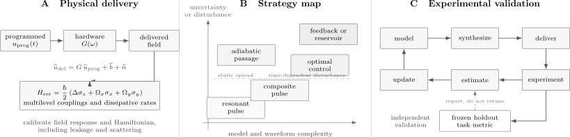
An AMO control protocol connects three levels of reasoning. A: a programmed waveform passes through hardware before defining a rotating-frame Hamiltonian. B: pulse, composite, adiabatic, optimal, and feedback methods address different uncertainty and time-scale regimes. C: model, synthesis, delivery, experiment, estimation, and update form a closed validation loop; task-level data must remain separate from the data used to tune the control.

Identifiability matters

Several parameter changes can produce similar observations. A reduced Rabi contrast may arise from detuning, amplitude inhomogeneity, state-preparation error, readout error, leakage, or decoherence. A single population trace cannot generally distinguish them. Useful calibration experiments vary independent knobs:

• pulse duration and amplitude to reveal coherent frequency;
• drive detuning to produce a chevron;
• phase to identify quadrature signs and imbalance;
• waiting time to separate coherent error from relaxation;
• spatial position or motional state to expose inhomogeneity;
• sequence length to amplify small coherent errors; and
• prepared input state and measurement basis to identify axis errors.

Parameter fitting is not validation when the same data both determine the model and establish its claimed accuracy.

Pulses and Pulse Areas

Resonant rotations

For $\Delta=0$ and constant phase, Hamiltonians at different times commute:

$$\left[ H_{\mathrm{rot}}(t), H_{\mathrm{rot}}(t') \right] = 0.$$

The propagator depends only on the signed pulse area

$$\Theta = \int_{t_i}^{t_f} \Omega(t)\,dt,$$

and is

$$R_\phi(\Theta) = \exp \left[ -\frac{i\Theta}{2} \left( \cos\phi\,\sigma_x + \sin\phi\,\sigma_y \right) \right].$$

A $\pi$ pulse swaps the two basis-state populations up to phases. A $\pi/2$ pulse creates an equal superposition, but the relative phase depends on $\phi$ and on the adopted basis convention. The pulse-area statement fails when detuning, phase, or the rotation axis changes during the pulse, because the Hamiltonians need not commute.

Worked Gaussian pulse audit

Consider a Gaussian envelope

$$\Omega(t) = \Omega_0 \exp \left[ -\frac{(t-t_0)^2}{2\sigma^2} \right].$$

If the pulse is integrated over a range much wider than $\sigma$,

$$\Theta \simeq \Omega_0\sigma\sqrt{2\pi}.$$

A nominal $\pi$ pulse therefore requires

$$\frac{\Omega_0}{2\pi} = \frac{1}{ 2\sigma\sqrt{2\pi} }.$$

For $\sigma=2.00\ \mu\mathrm{s}$,

$$\frac{\Omega_0}{2\pi} = 99.7\ \mathrm{kHz}.$$

This number is an infinite-support estimate. Truncating the pulse at $t_0\pm 2\sigma$ retains only

$$\operatorname{erf} \left( \frac{2}{\sqrt{2}} \right) \simeq 0.9545$$

of the area. The programmed peak must then be increased by about $4.77\%$ if all other assumptions remain valid. A waveform report that gives $\Omega_0$ and $\sigma$ but not the truncation convention is incomplete.

Detuning and noncommuting errors

For a rectangular pulse with constant $\Omega$, phase zero, and detuning $\Delta$, define

$$\Omega_R = \sqrt{\Omega^2+\Delta^2}.$$

Starting in $|g\rangle$,

$$P_e(t) = \frac{\Omega^2}{\Omega_R^2} \sin^2 \left( \frac{\Omega_Rt}{2} \right).$$

Suppose $\Omega/2\pi=100\ \mathrm{kHz}$ and $\Delta/2\pi=20\ \mathrm{kHz}$. A resonant calibration would choose $t_\pi=5.00\ \mu\mathrm{s}$. At that duration,

$$P_e(t_\pi) = \frac{1}{1+0.2^2} \sin^2 \left[ \frac{\pi}{2} \sqrt{1+0.2^2} \right] \simeq 0.9606.$$

The loss is mainly the tilt of the rotation axis, not a wrong pulse area. Stretching the pulse alone cannot make the maximum transfer exceed

$$P_{e,\max} = \frac{\Omega^2}{\Omega^2+\Delta^2} \simeq 0.9615.$$

Amplitude and phase errors

Let a nominal rotation $R_\phi(\Theta)$ experience a common fractional amplitude error $\epsilon$. The actual angle is

$$\Theta_{\mathrm{act}} = (1+\epsilon)\Theta.$$

For a nominal $\pi$ pulse applied to $|g\rangle$,

$$1-P_e = \sin^2 \left( \frac{\pi\epsilon}{2} \right) = \frac{\pi^2}{4}\epsilon^2 + O(\epsilon^4).$$

A $5\%$ amplitude error therefore gives an idealized transfer error

$$1-P_e \simeq 6.16\times10^{-3}.$$

This quadratic population error should not be confused with the coherent unitary error amplitude, which is first order in $\epsilon$ and can accumulate coherently in a longer sequence.

A constant phase offset rotates the control axis in the equatorial plane. If every pulse and every analysis operation shares the same offset, some measurements are insensitive to it. Relative phase errors between pulses, between sites, or between control and local oscillator are observable and often more consequential.

Spectral selectivity

A pulse of duration $\tau$ necessarily has a finite spectral width. A rectangular envelope produces sinc-like sidelobes, while smooth envelopes reduce abrupt high-frequency content. Selectivity is not determined by duration alone; it depends on the complete complex envelope and on the matrix elements of unwanted transitions.

For a leakage transition detuned by $\Delta_L$, a rough weak-drive scale is

$$P_{\mathrm{leak}} \sim \left| \frac{\Omega_L}{\Delta_L} \right|^2,$$

away from pulse-spectrum zeros and assuming negligible coherent return. Faster control raises $\Omega_L$ and can therefore conflict with state selectivity. Shaping redistributes the error; it does not repeal the bandwidth constraint.

Rotating Frames

Removing the carrier

Consider a laboratory Hamiltonian

$$H_{\mathrm{lab}}(t) = \frac{\hbar\omega_0}{2}\sigma_z + \hbar\Omega_d(t) \cos \left[ \omega_dt+\phi(t) \right] \sigma_x.$$

Choose

$$R(t) = \exp \left( -\frac{i\omega_dt}{2}\sigma_z \right),$$

and define the rotating-frame state

$$|\psi_{\mathrm{rot}}\rangle = R^\dagger(t)|\psi_{\mathrm{lab}}\rangle.$$

The transformed Hamiltonian is

$$H_{\mathrm{rot}} = R^\dagger H_{\mathrm{lab}}R - i\hbar R^\dagger\dot R.$$

After discarding terms oscillating near $2\omega_d$ under the rotating-wave approximation,

$$H_{\mathrm{rot}}(t) \simeq \frac{\hbar}{2} \left[ \Delta\sigma_z + \Omega_d(t) \cos\phi\,\sigma_x - \Omega_d(t) \sin\phi\,\sigma_y \right],$$

where $\Delta=\omega_0-\omega_d$ for this transformation and phase convention. The sign of the $\sigma_y$ term changes under other common definitions. An experimental document should state the convention or specify control axes operationally.

The rotating-wave approximation is a model reduction

Dropping the counter-rotating term requires more than a slowly drawn envelope. A representative condition is

$$|\Omega_d|, \ |\Delta|, \ \left|\frac{\dot\Omega_d}{\Omega_d}\right|, \ |\dot\phi| \ll \omega_0+\omega_d,$$

with care near envelope zeros. Strong or ultrafast drives produce counter-rotating effects, including a Bloch–Siegert shift of scale

$$\delta_{\mathrm{BS}} \sim \frac{\Omega_d^2}{4\omega_0}$$

for a near-resonant, weak sinusoidal drive, up to convention-dependent factors. In multilevel atoms, additional near-resonant transitions can fail before the two-level counter-rotating term becomes important.

Frequency and phase modulation

If the control phase is time dependent, the instantaneous drive frequency is shifted. Writing the laboratory phase as

$$\Phi_d(t) = \omega_{\mathrm{ref}}t+\phi(t),$$

gives

$$\omega_d(t) = \dot\Phi_d(t) = \omega_{\mathrm{ref}}+\dot\phi(t).$$

Phase ramps and frequency offsets are therefore two descriptions of the same operation. A discontinuity in the digital phase may be a deliberate axis jump, while a discontinuity in phase derivative is a frequency jump. Hardware that resets oscillator phase between pulses can silently change the intended sequence.

A frame dictionary

No single frame is best for every question:

Frame	Transformation removes	Best use	Main caution
Laboratory	nothing	physical frequencies, polarization, hardware phase	carrier obscures slow dynamics
Interaction	selected drift $H_0$	perturbation theory and resonant terms	depends on the chosen partition
Rotating	carrier or local oscillator	pulse axes, detuning, Rabi dynamics	signs and phase conventions vary
Toggling	applied control propagator	error averaging and dynamical decoupling	control imperfections also transform
Dressed	strong static or periodic drive	protected states, Autler–Townes structure	preparation and measurement must be mapped back
Adiabatic	instantaneous eigenbasis	passage and ramps	frame coupling $-i\hbar V^\dagger\dot V$ drives nonadiabatic transitions

For a general unitary frame transformation $V(t)$ with $|\widetilde\psi\rangle=V^\dagger|\psi\rangle$,

$$\widetilde H = V^\dagger HV - i\hbar V^\dagger\dot V.$$

The second term is not optional. It is the source of detuning terms in rotating frames and nonadiabatic couplings in instantaneous eigenbases.

Open systems in a new frame

For a master equation, the jump operators transform too:

$$\widetilde L_k(t) = V^\dagger(t)L_kV(t).$$

A frame change cannot remove physical decoherence. It can make a noise operator time dependent and reveal which spectral components drive transitions between dressed states. Leaving $L_k$ unchanged while transforming only $H$ generally defines a different model.

Adiabatic Passage

Following an instantaneous eigenstate

For the two-level Hamiltonian

$$H(t) = \frac{\hbar}{2} \left[ \Delta(t)\sigma_z + \Omega(t)\sigma_x \right],$$

define

$$\Omega_R(t) = \sqrt{\Delta^2(t)+\Omega^2(t)}$$

and a mixing angle satisfying

$$\tan\theta(t) = \frac{\Omega(t)}{\Delta(t)}.$$

The instantaneous eigenstates point parallel and antiparallel to

$$\mathbf h(t) = \left( \Omega(t),0,\Delta(t) \right)$$

on the Bloch sphere. Sweeping $\Delta$ from large negative to large positive values while keeping a nonzero gap can invert the population by following one eigenstate.

In the instantaneous eigenbasis, the geometric coupling has scale

$$\frac{|\dot\theta|}{2},$$

while the eigenfrequency gap is $\Omega_R$. A useful local condition is

$$|\dot\theta| \ll \Omega_R.$$

Equivalently,

$$\left| \Delta\dot\Omega-\Omega\dot\Delta \right| \ll \left( \Delta^2+\Omega^2 \right)^{3/2}.$$

The condition must hold where the gap is smallest, not only at the beginning and end.

Linear chirp and the Landau–Zener estimate

For constant $\Omega$ and a linear sweep

$$\Delta(t) = \alpha t$$

extended far beyond the avoided crossing, the ideal Landau–Zener diabatic-transition probability in this convention is

$$P_{\mathrm D} = \exp \left( -\frac{\pi\Omega^2}{2|\alpha|} \right).$$

The dimensionless ratio

$$\Lambda = \frac{\Omega^2}{|\alpha|}$$

is therefore a useful first audit. For a target $P_{\mathrm D}\le 10^{-3}$,

$$\Lambda \ge \frac{2\ln 10^3}{\pi} \simeq 4.40.$$

Finite sweep endpoints, envelope turn-on, decoherence, field inhomogeneity, and extra levels can dominate before this asymptotic formula is accurate.

STIRAP and dark-state passage

STIRAP uses an instantaneous dark state in a three-level system rather than a single avoided crossing. A Stokes pulse precedes and overlaps a pump pulse so that adiabatic following maps the initial state to the target while ideally suppressing occupation of a lossy intermediate state. Its robustness is structured:

• common amplitude variations can preserve the path while changing the adiabatic margin;
• two-photon detuning can directly destroy the dark state;
• finite pulse overlap creates nonadiabatic loss;
• optical phase noise changes transferred coherence; and
• multilevel couplings and differential light shifts modify the nominal three-state Hamiltonian.

The complete derivation and error analysis are at STIRAP.

Robustness, time, and dissipation

Adiabatic passage trades sensitivity to some pulse details for longer exposure and larger integrated control action. If a lossy state has instantaneous occupation $p_\ell(t)$ and decay rate $\Gamma_\ell(t)$, a small-loss estimate is

$$P_{\mathrm{loss}} \simeq \int_0^T \Gamma_\ell(t)p_\ell(t)\,dt.$$

Making a protocol slower can reduce nonadiabatic transitions while increasing this integral. The optimum duration is finite whenever both effects matter.

Shortcuts to adiabaticity add controls or redesign schedules so that the desired endpoint is reached faster. They are not free: the auxiliary Hamiltonian may require an unavailable operator, greater amplitude, additional bandwidth, or more accurate calibration. A shortcut should be evaluated against the same delivered-control and decoherence constraints as any other pulse.

Composite Pulses

Error cancellation by noncommuting rotations

A composite pulse replaces one intended rotation by a sequence of rotations with chosen phases and angles. Each constituent pulse suffers an error, but the error rotations point along different axes and can cancel order by order.

Write an ideal equatorial rotation as

$$R_\phi(\theta) = \exp \left[ -\frac{i\theta}{2} \sigma_\phi \right],$$

where

$$\sigma_\phi = \cos\phi\,\sigma_x + \sin\phi\,\sigma_y.$$

Under a common fractional pulse-length error $\epsilon$,

$$\widetilde R_\phi(\theta) = R_\phi \left[ (1+\epsilon)\theta \right].$$

The sequence is designed so that its ideal product gives the target and the first several terms in the error expansion vanish.

BB1 for amplitude error

One symmetric BB1 implementation of a target $x$ rotation $R_0(\theta)$ executes the following pulses in the listed time order:

$$R_0\left(\frac{\theta}{2}\right), \quad R_\phi(\pi), \quad R_{3\phi}(2\pi), \quad R_\phi(\pi), \quad R_0\left(\frac{\theta}{2}\right),$$

with

$$\phi = \arccos \left( -\frac{\theta}{4\pi} \right).$$

For a target $\theta=\pi$,

$$\phi = \arccos \left( -\frac{1}{4} \right) \simeq 104.48^\circ,$$

and $3\phi$ may be reduced modulo $360^\circ$.

In the ideal limit, the middle $\pi$–$2\pi$–$\pi$ correction block is an identity up to global phase. Under a common small amplitude error, its error rotation cancels the leading error of the target pulse. The residual propagator error begins at order $\epsilon^3$, so the small-error infidelity begins at order $\epsilon^6$. A primitive pulse has infidelity of order $\epsilon^2$.

This asymptotic statement is not a universal guarantee. BB1 is much longer than a primitive pulse:

$$\Theta_{\mathrm{tot}} = |\theta|+4\pi.$$

For a $\pi$ target, it accumulates five times the absolute rotation angle. It can therefore suffer more decoherence, off-resonant excitation, time-dependent noise, phase-transient error, and hardware distortion.

Error model determines the sequence

Composite-pulse families target different errors:

Dominant error	Representative strategy	What must be checked
Common pulse-length or amplitude error	BB1, SK1, broadband sequences	phase accuracy, detuning sensitivity, duration
Static detuning or off-resonance error	CORPSE-type sequences	amplitude error, finite bandwidth, sign convention
Simultaneous systematic errors	concatenated or numerically designed sequences	sequence length and cross terms
Spatial selectivity	narrowband or passband sequences	profile over the full spatial distribution
Time-dependent noise	filter-designed control or dynamically corrected gates	noise spectrum and pulse imperfections

A sequence robust to static amplitude error need not reject rapid amplitude noise. The former is an ensemble or calibration uncertainty; the latter is a stochastic process with a spectrum. These require different objective functions.

How to validate a composite pulse

Testing only at zero imposed error cannot show robustness. A useful experiment measures a response surface over deliberately varied amplitude and detuning:

$$F_{\mathrm{exp}} = F_{\mathrm{exp}} \left( \epsilon,\Delta \right).$$

The validation range should be declared before tuning. Compare the composite and primitive pulse at equal target, using:

• the same preparation and readout correction;
• confidence intervals from repeated trials;
• a duration-matched control when decoherence is important;
• a holdout set of amplitudes and detunings not used for calibration; and
• leakage-sensitive measurements, not only target population.

A broader plateau in a one-dimensional parameter scan does not establish robustness to all relevant errors.

Optimal Control Overview

Turning a physical task into an objective

Numerical optimal control searches over parameterized waveforms rather than choosing from a small analytic family. A representative objective is

$$J[\mathbf u] = 1-F[\mathbf u] + \lambda_A \sum_j \int_0^T |u_j(t)|^2\,dt + \lambda_S \sum_j \int_0^T |\dot u_j(t)|^2\,dt + \lambda_L L[\mathbf u].$$

The terms can penalize infidelity, control energy, slew or bandwidth, and leakage. Hard constraints may be more appropriate than penalties:

$$|u_j(t)|\le u_{j,\max}, \qquad |\dot u_j(t)|\le s_{j,\max}.$$

Changing the weights changes the question. A pulse described as “optimal” is meaningful only after the objective, constraints, model, duration, and optimization method are stated.

Piecewise-constant propagation

In a common discretization, each control is constant in $N$ intervals of duration $\Delta t$. The propagator is

$$U(T) = U_NU_{N-1}\cdots U_1,$$

with

$$U_n = \exp \left[ -\frac{i\Delta t}{\hbar} \left( H_0+\sum_j u_{j,n}H_j \right) \right].$$

Gradient methods such as GRAPE reuse forward and backward partial propagators to compute derivatives efficiently. Krotov-type methods update controls using forward and adjoint states while enforcing a monotonic improvement property under their assumptions. Basis methods such as CRAB optimize a lower-dimensional waveform expansion. The canonical algorithmic discussion is at Optimal Control.

Robust and ensemble objectives

Let $\boldsymbol{\xi}$ label detuning, intensity scale, position, motional occupation, transfer-function parameters, or other uncertain quantities. An average robust objective is

$$\overline F = \int p(\boldsymbol{\xi}) F(\boldsymbol{\xi})\, d\boldsymbol{\xi},$$

approximated by a weighted sample

$$\overline F \simeq \sum_{r=1}^{N_\xi} w_rF(\boldsymbol{\xi}_r).$$

This is appropriate when $p(\boldsymbol{\xi})$ is a justified operating distribution. A worst-case objective,

$$F_{\min} = \min_{\boldsymbol{\xi}\in\Xi} F(\boldsymbol{\xi}),$$

protects the weakest point in a declared set $\Xi$ but is harder to optimize. A tail-risk objective can interpolate between mean and strict worst case.

Correlations matter. Laser intensity and AC Stark shift may vary together; trap depth, motional frequency, and thermal occupation may not be independent. Sampling each parameter independently can optimize for unphysical combinations while missing the actual uncertainty manifold.

Model-based and closed-loop optimization

Three workflows are common:

1. Open-loop model-based design: optimize in a calibrated model, then deploy the waveform.
2. Model-assisted calibration: optimize in simulation, then tune a small number of correction parameters experimentally.
3. Closed-loop experimental optimization: use measured task performance directly as the objective and update waveform parameters.

Closed-loop optimization can compensate unknown static distortions, but it does not eliminate experimental design. The measured objective can be noisy, biased by readout, or insensitive to leakage. The optimizer may exploit a detector artifact or a parameter drift. Safety constraints, holdout tests, and an independently defined success metric remain necessary.

Controllability is not pulse quality

Lie-algebraic controllability asks whether the available Hamiltonians can generate a desired set of unitaries in an ideal model with sufficient time and admissible controls. It does not answer:

• how long the operation takes;
• how much amplitude or bandwidth it requires;
• whether it is robust;
• whether decoherence destroys it;
• whether the waveform is identifiable from measurements; or
• whether the hardware can deliver it.

Controllability is a reachability statement, not an experimental fidelity claim.

Decoherence, Leakage, and Robustness

A control error budget

It is useful to separate at least five classes of error:

$$\epsilon_{\mathrm{task}} \sim \epsilon_{\mathrm{coh}} + \epsilon_{\mathrm{diss}} + \epsilon_{\mathrm{leak}} + \epsilon_{\mathrm{SPAM}} + \epsilon_{\mathrm{model}},$$

only as a bookkeeping mnemonic. These contributions generally do not add linearly; coherent errors interfere, leakage can return, and SPAM can bias the inferred dynamics. The classes are:

• coherent control error: amplitude, phase, detuning, timing, crosstalk, and unwanted Hamiltonian terms;
• dissipative error: spontaneous emission, relaxation, dephasing, heating, and particle loss;
• leakage: population outside the declared computational or target manifold;
• SPAM error: imperfect state preparation and measurement; and
• model error: omitted levels, wrong transfer function, parameter drift, and invalid approximations.

Each requires a different diagnostic.

Relaxation during a pulse

Suppose a resonant $\pi$ pulse has duration $t_\pi=5.00\ \mu\mathrm{s}$ and the excited state relaxes with $T_1=1.00\ \mathrm{ms}$. For an ideal resonant rotation from the ground state,

$$p_e(t) = \sin^2 \left( \frac{\pi t}{2t_\pi} \right),$$

whose time average is $1/2$. A first-order jump estimate is

$$P_{\mathrm{jump}} \simeq \int_0^{t_\pi} \frac{p_e(t)}{T_1}\,dt = \frac{t_\pi}{2T_1} = 2.50\times10^{-3}.$$

This is already comparable to the primitive-pulse error from a few-percent amplitude miscalibration. A five-times-longer composite sequence may greatly suppress the systematic amplitude error while accumulating a larger relaxation contribution. The crossover must be calculated, not assumed.

Spontaneous scattering in Raman control

For a simplified far-detuned three-level Raman process, effective coupling and scattering scale schematically as

$$\Omega_{\mathrm{eff}} \sim \frac{\Omega_1\Omega_2^*}{2\Delta},$$ $$\Gamma_{\mathrm{sc}} \sim \Gamma \frac{ |\Omega_1|^2+|\Omega_2|^2 }{4\Delta^2},$$

with multilevel sums and convention-dependent factors in real atoms. Increasing $|\Delta|$ suppresses scattering at fixed single-photon Rabi frequencies but also slows the coherent process. Holding $\Omega_{\mathrm{eff}}$ fixed requires more optical intensity and changes the scaling. Differential light shifts must be included in the same optimization.

Leakage and coherent return

Leakage is not always monotonic. An unwanted level may be transiently populated and coherently return by the end of a pulse. Endpoint leakage can therefore be small while transient occupation exposes the system to decay or creates sensitivity to timing. Useful metrics include

$$L_{\mathrm{end}} = 1- \operatorname{Tr} \left[ P\rho(T) \right],$$

and

$$L_{\mathrm{int}} = \int_0^T \left\{ 1- \operatorname{Tr} \left[ P\rho(t) \right] \right\} dt.$$

The first measures final leakage; the second is an exposure measure. Which one matters depends on whether leaked states decay, dephase, collide, or remain detectable.

Quasi-static uncertainty and stochastic noise

An uncertain but constant detuning during one shot should be modeled by an ensemble:

$$\rho(T) = \int p(\Delta) U_\Delta(T)\rho(0)U_\Delta^\dagger(T) \,d\Delta.$$

Rapid detuning noise requires a stochastic or open-system description. Two noise processes with the same variance but different spectra can respond very differently to a pulse sequence. Composite pulses, adiabatic passage, and dynamical decoupling cannot be ranked from a single root-mean-square noise number.

Robustness is multidimensional

A robust protocol should declare:

• the uncertain parameters and their joint range or distribution;
• which errors are static within a shot and which vary during it;
• the performance metric and acceptable threshold;
• the duration, amplitude, bandwidth, and energy constraints;
• the training or calibration points;
• the independent validation points; and
• the behavior outside the intended range.

Calling a pulse “robust” without these qualifiers is not an experimentally testable statement.

Choosing a Control Strategy

Method-selection map

The following map is a starting point, not a ranking:

Situation	First method to test	Why	Failure mode to audit
Well-isolated transition, accurate resonance, short task	resonant shaped pulse	simple, fast, interpretable	area, detuning, leakage
Dominant repeatable amplitude bias	composite pulse or robust shaped pulse	analytic or numerical cancellation	added duration and phase transients
Broad static detuning distribution	adiabatic rapid passage or robust optimization	follows a gapped eigenstate or trains over ensemble	long exposure and endpoint errors
Lossy intermediate state in a lambda system	STIRAP	dark-state pathway suppresses intermediate occupation	two-photon detuning and phase noise
Dense multilevel spectrum with several constraints	numerical optimal control	uses interference and full model	model mismatch and bandwidth
Slowly drifting hardware	model-assisted closed-loop calibration	updates a small parameter set	estimator bias and overfitting
Time-dependent dephasing noise	filter-designed control or dynamical decoupling	targets a noise spectrum	pulse errors and incompatible signal filtering
State stabilization under ongoing disturbance	measurement feedback or reservoir engineering	continuously removes deviations	latency, inefficiency, backaction

The simplest protocol that meets the task and validation requirements is usually easiest to maintain. Complexity is justified when it removes a measured limitation.

Time-scale hierarchy

Before selecting a method, compare

$$\tau_{\mathrm{carrier}}, \quad \tau_{\mathrm{rise}}, \quad \tau_{\mathrm{ctrl}}, \quad \tau_{\mathrm{noise}}, \quad T_2^*, \quad T_2, \quad T_1, \quad \tau_{\mathrm{drift}}.$$

Here $\tau_{\mathrm{rise}}$ characterizes hardware bandwidth, $\tau_{\mathrm{ctrl}}$ the protocol duration, $\tau_{\mathrm{noise}}$ a relevant noise correlation time, and $\tau_{\mathrm{drift}}$ the calibration lifetime. A typical coherent-control window seeks

$$\tau_{\mathrm{rise}} \ll \tau_{\mathrm{ctrl}} \ll T_1,T_2,$$

but selectivity, adiabaticity, and motional resolution may impose lower bounds on $\tau_{\mathrm{ctrl}}$. There is no universal preference for faster or slower.

Platform-specific constraints

The same mathematical pulse can encounter different physical limits:

• neutral atoms: Doppler shifts, differential light shifts, spatial intensity variation, atom loss, Rydberg decay, and site crosstalk;
• trapped ions: motional mode crowding, heating, residual spin–motion entanglement, optical phase, and spectator transitions;
• molecules: dense rovibrational structure, incomplete branching closure, tensor Stark shifts, and state-dependent loss;
• cavity QED: photon loss, cooperativity, cavity filtering, atomic transit, and measurement backaction;
• circuit QED: anharmonic leakage, microwave transfer functions, residual photons, crosstalk, and relaxation; and
• atom interferometers: laser phase noise, vibration, wavefront aberrations, momentum closure, and ensemble inhomogeneity.

The platform pages develop these constraints in their physical context.

Calibration and Validation

A calibration ladder

A defensible workflow moves from simple, identifiable tests to the final task:

1. Reference and timing: lock or measure oscillator frequencies, clock alignment, trigger latency, and phase-reset behavior.
2. Hardware response: measure gain, phase, impulse response, compression, switching transients, and crosstalk over the used amplitude and frequency range.
3. Hamiltonian primitives: use spectroscopy, Rabi oscillations, Ramsey fringes, and chevrons to estimate detuning, coupling, phase axes, and coherence.
4. Multilevel checks: search for leakage, spectator excitation, sidebands, light shifts, and power-dependent resonance shifts.
5. Sequence checks: amplify coherent errors with repeated pulses, echoes, phase cycles, or deliberately inserted error scans.
6. Task validation: measure the declared state, gate, sensing, or simulation metric on data not used to tune the control.
7. Drift monitoring: repeat compact sentinels and define recalibration thresholds.

Skipping directly to a high final population makes it difficult to know which assumption failed when performance drifts.

Training, validation, and stress tests

Separate data into three logical roles:

• calibration data estimate model and hardware parameters;
• training data tune a pulse or optimizer;
• validation data test the frozen protocol; and
• stress data probe outside the nominal operating region.

The first two may overlap in a carefully modeled workflow, but validation must remain independent enough to detect overfitting. For a robustness claim, predeclare the validation grid or distribution.

Uncertainty propagation

Suppose fitted parameters have posterior or sampling distribution $p(\boldsymbol{\xi}\mid D)$. Predictive control performance is then

$$p(F\mid D) = \int \delta \left[ F-F(\boldsymbol{\xi}) \right] p(\boldsymbol{\xi}\mid D) \,d\boldsymbol{\xi}.$$

Reporting only $F$ at the best-fit parameter values ignores calibration uncertainty. Monte Carlo propagation through the full control simulation is often more transparent than a local linear estimate when the response is nonlinear.

Task metrics and diagnostic metrics

A diagnostic metric should identify an error; a task metric should measure the intended use. Examples:

Diagnostic	Identifies	Does not by itself prove
Rabi chevron	coupling, detuning, asymmetry	gate fidelity
Ramsey fringe	relative phase and detuning	leakage-free control
population transfer	endpoint occupation	coherent phase preservation
process tomography	operation in tested basis set	performance under long sequences
randomized benchmarking	average sequence error under assumptions	worst-case coherent error or leakage details
robustness scan	sensitivity over chosen axes	robustness to omitted axes
task observable	end-use performance	microscopic error mechanism

Several complementary measurements are usually needed.

Reproducible control record

A mature control result should preserve:

• Hamiltonian and dissipative model, including basis ordering;
• frame, phase, and angular-frequency conventions;
• waveform samples or an exact parameterization;
• sample rate, truncation, interpolation, and synchronization;
• hardware transfer-function and predistortion version;
• amplitude, bandwidth, slew, and duration constraints;
• uncertainty distribution or robustness set;
• objective function and all weights;
• optimizer, initialization, stopping rule, and random seeds;
• calibration data and date;
• validation protocol, raw counts, uncertainty method, and holdout policy;
• leakage and SPAM treatment; and
• conditions that trigger recalibration.

This record turns a plotted pulse into a reproducible scientific object.

Common Mistakes

Treating the programmed envelope as the delivered field

Finite bandwidth, dispersion, mixers, resonators, and nonlinear amplifiers change amplitude and phase. Measure or bound the transfer function in the operating regime.

Mixing hertz and radians per second

The error is a factor of $2\pi$ in pulse times, chirp rates, and adiabaticity parameters. State conventions near the first equation and carry units through numerical audits.

Using pulse area off resonance

Area alone determines a rotation only for a fixed resonant axis. Detuning tilts the axis; time-dependent phase and multilevel coupling make Hamiltonians at different times noncommuting.

Omitting the frame derivative

Under $V(t)$, the Hamiltonian is $V^\dagger HV-i\hbar V^\dagger\dot V$. The derivative term creates detuning and nonadiabatic couplings.

Transforming the Hamiltonian but not the noise

Jump and noise operators also transform. Keeping them fixed can change the physical model.

Calling adiabatic passage insensitive

Adiabatic methods are insensitive to some waveform variations only when the gap, endpoint, detuning, phase, and dissipation requirements remain satisfied.

Calling one composite sequence robust

BB1 targets a common pulse-length error. It does not automatically correct detuning, stochastic noise, phase transients, leakage, or decoherence.

Optimizing an incomplete objective

A high projected-subspace overlap can hide leakage. A high state-transfer fidelity can hide wrong action on other inputs. Penalties and constraints must reflect the physical task.

Training and testing on the same scan

The optimizer can fit noise or a readout artifact. Freeze the protocol and evaluate independent validation points.

Reporting simulation fidelity as experimental fidelity

Simulation validates code against a model. Experiment tests the model, hardware, preparation, control, and measurement together.

Assuming the longest coherence time sets the control limit

Leakage spacing, spontaneous scattering, motional heating, bandwidth, crosstalk, and drift can dominate even when $T_1$ and $T_2$ are long.

Key Results

For a resonant fixed-axis pulse,

$$R_\phi(\Theta) = \exp \left[ -\frac{i\Theta}{2} \left( \cos\phi\,\sigma_x + \sin\phi\,\sigma_y \right) \right], \qquad \Theta=\int\Omega(t)\,dt.$$

For a time-dependent unitary frame,

$$\widetilde H = V^\dagger HV - i\hbar V^\dagger\dot V, \qquad \widetilde L_k = V^\dagger L_kV.$$

For a two-level adiabatic passage,

$$\left| \Delta\dot\Omega-\Omega\dot\Delta \right| \ll \left( \Delta^2+\Omega^2 \right)^{3/2}.$$

For a linear Landau–Zener sweep in the stated convention,

$$P_{\mathrm D} = \exp \left( -\frac{\pi\Omega^2}{2|\dot\Delta|} \right).$$

For BB1 amplitude compensation,

$$\phi = \arccos \left( -\frac{\theta}{4\pi} \right),$$

and the small common-amplitude-error infidelity scales as $O(\epsilon^6)$ rather than $O(\epsilon^2)$, at the cost of a longer sequence.

For robust optimal control,

$$\overline F = \int p(\boldsymbol{\xi}) F(\boldsymbol{\xi})\,d\boldsymbol{\xi},$$

but a trustworthy result also requires delivered-waveform calibration, leakage and decoherence modeling, and independent task-level validation.

Further Connections

• Rabi Oscillations develops pulse areas, detuned rotations, chevrons, and Rabi diagnostics.
• Ramsey Interferometry develops phase-coherent separated-pulse control.
• Optical Bloch Equations connects coherent drive to relaxation and dephasing.
• STIRAP gives the canonical three-state adiabatic-passage derivation.
• Trapped-Ion Control applies these ideas to internal states and collective motion.
• Rydberg Blockade applies them to interacting neutral-atom gates and many-body dynamics.
• Circuit QED Overview maps microwave synthesis, dispersive readout, and calibration onto artificial atoms.
• Atom Interferometry uses phase-coherent pulses as matter-wave beam splitters and mirrors.
• Pulse Sequences defines standard sequence notation and echo families.
• Driven Open Systems gives the canonical time-dependent master-equation framework.
• Dynamical Decoupling treats toggling frames and spectral noise filtering.
• Optimal Control develops objectives, gradients, GRAPE, Krotov methods, and validation.
• Control Limits and Noise develops bandwidth, leakage, speed, drift, and measurement limits.
• Measurement-Based Feedback treats causal state estimation and feedback stabilization.

References

1. B. W. Shore, Manipulating Quantum Structures Using Laser Pulses (Cambridge University Press, 2011), doi:10.1017/CBO9780511844222.
2. C. Cohen-Tannoudji, J. Dupont-Roc, and G. Grynberg, Atom–Photon Interactions: Basic Processes and Applications (Wiley, 1992).
3. L. M. K. Vandersypen and I. L. Chuang, “NMR techniques for quantum control and computation,” Reviews of Modern Physics 76, 1037–1069 (2005), doi:10.1103/RevModPhys.76.1037.
4. N. V. Vitanov, A. A. Rangelov, B. W. Shore, and K. Bergmann, “Stimulated Raman adiabatic passage in physics, chemistry, and beyond,” Reviews of Modern Physics 89, 015006 (2017), doi:10.1103/RevModPhys.89.015006.
5. K. Bergmann, H. Theuer, and B. W. Shore, “Coherent population transfer among quantum states of atoms and molecules,” Reviews of Modern Physics 70, 1003–1025 (1998), doi:10.1103/RevModPhys.70.1003.
6. D. Guéry-Odelin, A. Ruschhaupt, A. Kiely, E. Torrontegui, S. Martínez-Garaot, and J. G. Muga, “Shortcuts to adiabaticity: concepts, methods, and applications,” Reviews of Modern Physics 91, 045001 (2019), doi:10.1103/RevModPhys.91.045001.
7. M. H. Levitt, “Composite pulses,” Progress in Nuclear Magnetic Resonance Spectroscopy 18, 61–122 (1986), doi:10.1016/0079-6565(86)80005-X.
8. S. Wimperis, “Broadband, narrowband, and passband composite pulses for use in advanced NMR experiments,” Journal of Magnetic Resonance, Series A 109, 221–231 (1994), doi:10.1006/jmra.1994.1159.
9. H. K. Cummins, G. Llewellyn, and J. A. Jones, “Tackling systematic errors in quantum logic gates with composite rotations,” Physical Review A 67, 042308 (2003), doi:10.1103/PhysRevA.67.042308.
10. K. R. Brown, A. W. Harrow, and I. L. Chuang, “Arbitrarily accurate composite pulse sequences,” Physical Review A 70, 052318 (2004), doi:10.1103/PhysRevA.70.052318.
11. N. Khaneja, T. Reiss, C. Kehlet, T. Schulte-Herbrüggen, and S. J. Glaser, “Optimal control of coupled spin dynamics: design of NMR pulse sequences by gradient ascent algorithms,” Journal of Magnetic Resonance 172, 296–305 (2005), doi:10.1016/j.jmr.2004.11.004.
12. J. P. Palao and R. Kosloff, “Quantum computing by an optimal control algorithm for unitary transformations,” Physical Review Letters 89, 188301 (2002), doi:10.1103/PhysRevLett.89.188301.
13. S. J. Glaser et al., “Training Schrödinger’s cat: quantum optimal control,” European Physical Journal D 69, 279 (2015), doi:10.1140/epjd/e2015-60464-1.
14. R. S. Judson and H. Rabitz, “Teaching lasers to control molecules,” Physical Review Letters 68, 1500–1503 (1992), doi:10.1103/PhysRevLett.68.1500.
15. S. van Frank et al., “Optimal control of complex atomic quantum systems,” Scientific Reports 6, 34187 (2016), doi:10.1038/srep34187.
16. J. Kelly et al., “Optimal quantum control using randomized benchmarking,” Physical Review Letters 112, 240504 (2014), doi:10.1103/PhysRevLett.112.240504.
17. C. Kabytayev, T. J. Green, K. Khodjasteh, M. J. Biercuk, L. Viola, and K. R. Brown, “Robustness of composite pulses to time-dependent control noise,” Physical Review A 90, 012316 (2014), doi:10.1103/PhysRevA.90.012316.
18. H. J. Metcalf and P. van der Straten, Laser Cooling and Trapping (Springer, 1999), doi:10.1007/978-1-4612-1470-0.
19. D. Leibfried, R. Blatt, C. Monroe, and D. Wineland, “Quantum dynamics of single trapped ions,” Reviews of Modern Physics 75, 281–324 (2003), doi:10.1103/RevModPhys.75.281.
20. M. Saffman, T. G. Walker, and K. Mølmer, “Quantum information with Rydberg atoms,” Reviews of Modern Physics 82, 2313–2363 (2010), doi:10.1103/RevModPhys.82.2313.

Exercises

1. Audit a truncated Gaussian pulse

A Gaussian Rabi envelope is

$$\Omega(t) = \Omega_0 \exp \left( -\frac{t^2}{2\sigma^2} \right)$$

and is truncated to $|t|\le 2\sigma$.

1. Derive the retained fraction of the infinite-support pulse area.
2. Find $\Omega_0/2\pi$ for a truncated $\pi$ pulse with $\sigma=2.00\ \mu\mathrm{s}$.
3. Explain why matching the area is not sufficient if a constant detuning is present.

Solution

The truncated area is

$$\Theta_{\mathrm{tr}} = \Omega_0 \int_{-2\sigma}^{2\sigma} \exp \left( -\frac{t^2}{2\sigma^2} \right) dt.$$

With $x=t/(\sqrt{2}\sigma)$,

$$\Theta_{\mathrm{tr}} = \Omega_0\sigma\sqrt{2\pi} \operatorname{erf} \left( \sqrt{2} \right).$$

The retained fraction is

$$f_2 = \operatorname{erf} \left( \sqrt{2} \right) \simeq 0.95450.$$

Setting $\Theta_{\mathrm{tr}}=\pi$ gives

$$\frac{\Omega_0}{2\pi} = \frac{1}{ 2\sigma\sqrt{2\pi}f_2 }.$$

For $\sigma=2.00\ \mu\mathrm{s}$,

$$\frac{\Omega_0}{2\pi} \simeq 104.5\ \mathrm{kHz}.$$

With detuning, the rotation axis has a nonzero $z$ component. Hamiltonians with a shaped transverse amplitude and constant detuning generally do not commute at different times, so the final propagator is not determined by the transverse area alone.

2. Compare nominal and detuned pi pulses

A square pulse is calibrated with $\Omega/2\pi=100\ \mathrm{kHz}$ and applied for $t_\pi=5.00\ \mu\mathrm{s}$. During the experiment, $\Delta/2\pi=20.0\ \mathrm{kHz}$.

1. Find the generalized Rabi frequency.
2. Calculate the excited-state probability at $t_\pi$.
3. Find the largest excited-state probability possible without correcting the detuning.
4. Identify a calibration scan that can distinguish detuning from a simple amplitude error.

Solution

The generalized angular frequency is

$$\Omega_R = \sqrt{\Omega^2+\Delta^2},$$

so

$$\frac{\Omega_R}{2\pi} = \sqrt{ (100\ \mathrm{kHz})^2 + (20.0\ \mathrm{kHz})^2 } = 102.0\ \mathrm{kHz}.$$

At the nominal pulse time,

$$P_e = \frac{\Omega^2}{\Omega_R^2} \sin^2 \left( \frac{\Omega_Rt_\pi}{2} \right) = \frac{1}{1.04} \sin^2 \left( \frac{\pi}{2}\sqrt{1.04} \right) \simeq 0.9606.$$

The maximum is the prefactor,

$$P_{e,\max} = \frac{1}{1.04} \simeq 0.9615.$$

A two-dimensional Rabi chevron that scans both drive frequency and pulse duration identifies the resonance center and separates detuning from the on-resonance coupling. A duration scan at only one nominal frequency is more ambiguous.

3. Derive the adiabatic coupling

For

$$H = \frac{\hbar}{2} \left( \Delta\sigma_z+\Omega\sigma_x \right),$$

let

$$\tan\theta = \frac{\Omega}{\Delta}.$$

1. Show that $\dot\theta=(\Delta\dot\Omega-\Omega\dot\Delta)/ (\Delta^2+\Omega^2)$.
2. Compare the geometric coupling to the eigenfrequency gap.
3. For a linear sweep $\Delta=\alpha t$ and constant $\Omega$, state where the local adiabatic condition is hardest to satisfy.

Solution

Differentiate $\theta=\arctan(\Omega/\Delta)$:

$$\dot\theta = \frac{ \Delta\dot\Omega-\Omega\dot\Delta }{ \Delta^2+\Omega^2 }.$$

A rotation about $y$ diagonalizes the Hamiltonian. Its frame derivative produces an off-diagonal term of magnitude $\hbar|\dot\theta|/2$. The eigenenergy separation is $\hbar\Omega_R$, where

$$\Omega_R = \sqrt{\Delta^2+\Omega^2}.$$

Thus a local adiabatic requirement is

$$|\dot\theta| \ll \Omega_R,$$

or

$$\left| \Delta\dot\Omega-\Omega\dot\Delta \right| \ll \left( \Delta^2+\Omega^2 \right)^{3/2}.$$

For $\Delta=\alpha t$ and constant $\Omega$,

$$|\dot\theta| = \frac{|\alpha|\Omega}{ \alpha^2t^2+\Omega^2 }.$$

The geometric coupling is largest and the gap is smallest at the avoided crossing $t=0$. That is the hardest part of the sweep.

4. Construct a BB1 pi pulse

Use the symmetric BB1 sequence for a target $R_x(\pi)$.

1. Calculate the correction phase $\phi$.
2. List the pulse angles and phases in time order.
3. Find the total absolute rotation angle.
4. Explain why the sequence can perform worse than a primitive pulse even though its static amplitude-error scaling is better.

Solution

For $\theta=\pi$,

$$\phi = \arccos \left( -\frac{\theta}{4\pi} \right) = \arccos \left( -\frac14 \right) \simeq 104.48^\circ.$$

The pulses are, in time order,

$$R_0\left(\frac{\pi}{2}\right), \quad R_\phi(\pi), \quad R_{3\phi}(2\pi), \quad R_\phi(\pi), \quad R_0\left(\frac{\pi}{2}\right).$$

The phase $3\phi\simeq313.43^\circ$ after reduction modulo $360^\circ$. The total absolute angle is

$$\Theta_{\mathrm{tot}} = \frac{\pi}{2}+\pi+2\pi+\pi+\frac{\pi}{2} = 5\pi.$$

BB1 changes the small common amplitude-error infidelity from order $\epsilon^2$ to order $\epsilon^6$, but it is five times as long at fixed Rabi rate. Decoherence, detuning, phase transients, time-dependent noise, and leakage can then outweigh the static-amplitude benefit.

5. Decide when BB1 helps

Compare a primitive $\pi$ pulse with a BB1 $\pi$ pulse. Assume:

• the primitive static amplitude-error contribution is $c_2\epsilon^2$;
• the BB1 contribution is $c_6\epsilon^6$;
• both accumulate an incoherent error at constant rate $\gamma$ per unit absolute rotation angle; and
• BB1 has total angle $5\pi$ while the primitive has angle $\pi$.

1. Write approximate total errors for both.
2. Derive the inequality for BB1 to help.
3. Explain what experimental scan would test the model.

Solution

In this simplified additive model,

$$\varepsilon_{\mathrm{prim}} \simeq c_2\epsilon^2+\gamma\pi,$$

and

$$\varepsilon_{\mathrm{BB1}} \simeq c_6\epsilon^6+5\gamma\pi.$$

BB1 helps when

$$c_2\epsilon^2-c_6\epsilon^6 > 4\gamma\pi.$$

The left side is the coherent-error reduction; the right side is the added incoherent cost. The coefficients depend on the fidelity definition and sequence convention.

Experimentally, impose a calibrated range of amplitude scale errors and measure both protocols, including a duration-matched control and a leakage-sensitive readout. Repeating the sequence several times can amplify coherent residuals. A simultaneous detuning scan checks whether an apparent advantage is confined to one axis.

6. Build a robust-control objective

An optical transition has uncertain fractional intensity scale $s\in[0.9,1.1]$ and detuning $\Delta/2\pi\in[-20,20]\ \mathrm{kHz}$. Population can also leak into $|\ell\rangle$.

1. Propose a sampled average-fidelity objective.
2. Add a final-leakage penalty and a slew penalty.
3. State one reason to prefer a worst-case objective.
4. Give one correlation that independent sampling might miss.

Solution

Choose samples $(s_r,\Delta_r)$ with justified weights $w_r$. One objective to minimize is

$$J = 1- \sum_r w_rF(s_r,\Delta_r) + \lambda_L \sum_r w_r \langle\ell| \rho_r(T) |\ell\rangle + \lambda_S \sum_j \int_0^T |\dot u_j(t)|^2dt.$$

The weights should represent the operating distribution if average performance is the goal. A worst-case objective is useful when every atom, site, or operating point must exceed a threshold and a small bad tail is unacceptable.

Independent sampling could miss a correlation between intensity and AC Stark detuning, because both arise from the same optical field. It could also miss correlations among trap depth, motional frequency, temperature, and coupling.

7. Estimate dissipation during control

A resonant $\pi$ pulse lasts $5.00\ \mu\mathrm{s}$ and drives an excited state with lifetime $T_1=1.00\ \mathrm{ms}$.

1. Using the ideal excited-state trajectory, estimate the probability of a relaxation jump to first order.
2. Repeat the estimate for a sequence with the same average excited-state population but duration $25.0\ \mu\mathrm{s}$.
3. Why is this not a complete comparison between a primitive and composite pulse?

Solution

For a resonant primitive pulse,

$$p_e(t) = \sin^2 \left( \frac{\pi t}{2t_\pi} \right),$$

and

$$\int_0^{t_\pi} p_e(t)\,dt = \frac{t_\pi}{2}.$$

Thus

$$P_{\mathrm{jump}} \simeq \frac{t_\pi}{2T_1} = \frac{5.00\ \mu\mathrm{s}}{ 2(1.00\ \mathrm{ms}) } = 2.50\times10^{-3}.$$

For $25.0\ \mu\mathrm{s}$ with the same average population,

$$P_{\mathrm{jump}} \simeq 1.25\times10^{-2}.$$

The comparison is incomplete because a composite pulse has a different time-dependent state trajectory, not necessarily the same average excited population. Relaxation events can repopulate states, phase errors can interfere, and the longer sequence may also alter leakage, detuning sensitivity, and readout. A master-equation or trajectory simulation with the actual sequence is needed.

8. Design an independent validation campaign

A numerically optimized Raman pulse was trained in simulation over laser intensity and two-photon detuning, then adjusted experimentally using final target population.

Design a validation campaign that can support the claim:

The pulse transfers the coherent state across the declared operating range with at least $99\%$ fidelity.

Your answer should identify calibration data, holdout data, coherence and leakage diagnostics, uncertainty treatment, and a drift policy.

Solution

There is no unique campaign, but a defensible one includes the following.

First, freeze the pulse and all predistortion after training. Record the Hamiltonian model, waveform samples, hardware settings, and calibration timestamp. Predeclare a two-dimensional holdout grid or a random sample from the operating distribution that was not used for tuning.

At each holdout point, measure target population with independently calibrated state preparation and readout. Population alone does not prove coherent transfer, so insert an analysis pulse or Ramsey-type interference that tests the target phase relative to a reference. Measure populations in known leakage states or use a loss-aware readout. Include a primitive or analytic control as a baseline.

Use repeated binomial trials and propagate uncertainty in SPAM calibration, intensity, and detuning. Report pointwise confidence intervals and the predeclared aggregate metric, such as a lower confidence bound on the worst-case fidelity. Do not discard failed operating points after looking at the data.

Finally, define short sentinel experiments, for example a Rabi frequency, Ramsey detuning, Raman light shift, and leakage check. Recalibrate when a sentinel crosses a predeclared threshold or after a maximum elapsed time. The validation claim then applies only within that calibration regime.

Frontier Context

Molecular Control Frontiers tracks dated evidence and open claims in molecular STIRAP, coherent pathway interference, reaction selectivity, response-aware pulse design, and steering through nonadiabatic regions. The control models, objective design, calibration logic, robustness tests, and validation workflow developed here remain canonical.