Ion Traps

An ion trap confines charged particles with electromagnetic fields while preserving optical access to their internal states. In the most common AMO implementation, a radio-frequency Paul trap supplies dynamic transverse confinement, static electrodes confine the remaining direction, laser cooling reduces the secular motion, and state-dependent fluorescence reveals the internal state.

The compact description

$$\text{electrode voltages} \longrightarrow \text{Mathieu motion} \longrightarrow \text{secular oscillator} \longrightarrow \text{quantized modes}$$

contains several distinct approximations. The exact trajectory in a Paul trap is periodically driven. A time-independent harmonic pseudopotential is a controlled reduction of that dynamics, not the literal electric potential. The fast motion does not vanish when the slow secular motion is cold, and a fluorescing ion is not automatically known to occupy the motional ground state. Keeping those distinctions explicit is essential in precision spectroscopy, quantum information, and motional-state engineering.

Canonical Scope

This page owns the platform-level account of:

1. why static electric fields alone cannot produce a three-dimensional free-space minimum for a charged particle;
2. ideal quadrupole Paul traps, Mathieu parameters, stability, and the pseudopotential approximation;
3. secular motion, intrinsic micromotion, and excess micromotion;
4. linear RF traps with static axial confinement;
5. quantized single-ion motion and normal modes of Coulomb crystals;
6. internal-state encodings, loading, cooling, fluorescence measurement, and the calibrations that connect them;
7. a validity and error ledger for claims about confinement and preparation.

The general mathematics of periodically driven quantum systems belongs to Floquet Theory in Quantum Mechanics. The Quantum Harmonic Oscillator owns oscillator eigenstates, ladder operators, and phase-space structure. Laser Cooling and Doppler Cooling own their general force, diffusion, and temperature derivations.

The Trapped Ions application map owns the open-system description of fluorescence backaction, electric-field-noise heating, engineered dissipation, trajectories, and internal-state dephasing. Detailed carrier and sideband control, Lamb–Dicke expansions, and entangling gates belong to Trapped-Ion Control. Here they appear only as preparation and diagnostic tools. Trapped-Ion Qubits owns the processor-level account of encodings, connectivity, QCCD routing, photonic interconnects, and scaling.

Why Dynamic Confinement Is Needed

For a charge $Q$ in an electrostatic potential $\Phi(\mathbf r)$, the potential energy is

$$U(\mathbf r)=Q\Phi(\mathbf r).$$

In a charge-free trapping region, Laplace’s equation requires

$$\nabla^2\Phi=0.$$

At a putative smooth minimum of $\Phi$, all three principal curvatures would have to be positive, but their sum is $\nabla^2\Phi=0$. A static potential can focus a positive charge in one direction only by defocusing it in at least one other direction. Reversing the sign of $Q$ reverses maxima and minima but does not evade the argument. This is the electrostatic content of Earnshaw’s theorem.

There are two standard ways around the obstruction:

• a Paul trap uses a time-periodic electric quadrupole, so alternating focusing can be dynamically stable;
• a Penning trap combines a static electric quadrupole with a static magnetic field, so the Lorentz force supplies radial confinement.

Paul traps dominate laser-cooled quantum-control experiments because they can provide strong confinement without a large bias magnetic field. Penning traps remain indispensable for precision mass measurements, fundamental-particle studies, clocks, and rotating ion crystals. The remainder of this page focuses on linear Paul traps.

Ideal Quadrupole Paul Trap

Convention ledger

Consider an ideal two-dimensional quadrupole potential

$$\Phi(x,y,t) = \frac{U_{\mathrm{dc}}-V_{\mathrm{rf}}\cos(\Omega_{\mathrm{rf}}t)} {2r_0^2} \left(x^2-y^2\right).$$

The symbols mean:

Symbol	Meaning
$U_{\mathrm{dc}}$	static quadrupole voltage in this idealized model
$V_{\mathrm{rf}}$	zero-to-peak RF voltage, not peak-to-peak voltage
$\Omega_{\mathrm{rf}}$	RF angular drive frequency
$r_0$	characteristic electrode distance for the chosen potential convention
$Q,m$	ion charge and mass

Changing the sign or phase of the RF term changes intermediate signs but not the stability physics. Real electrodes introduce dimensionless geometry factors and higher multipoles. Therefore a voltage and electrode spacing do not define a trap frequency until the electrostatic model and voltage convention are stated.

Equations of motion

The electric field is $\mathbf E=-\boldsymbol{\nabla}\Phi$. Newton’s equation in the $x$ direction is

$$m\ddot{x} + \frac{Q}{r_0^2} \left[ U_{\mathrm{dc}} - V_{\mathrm{rf}}\cos(\Omega_{\mathrm{rf}}t) \right]x =0.$$

Introduce dimensionless time

$$\tau=\frac{\Omega_{\mathrm{rf}}t}{2}.$$

Then the transverse equations take Mathieu form,

$$\begin{aligned} \frac{d^2x}{d\tau^2} + \left(a_x-2q_x\cos 2\tau\right)x &=0, \\ \frac{d^2y}{d\tau^2} + \left(a_y-2q_y\cos 2\tau\right)y &=0, \end{aligned}$$

with

$$\begin{aligned} a_x &= \frac{4QU_{\mathrm{dc}}} {mr_0^2\Omega_{\mathrm{rf}}^2}, & q_x &= \frac{2QV_{\mathrm{rf}}} {mr_0^2\Omega_{\mathrm{rf}}^2}, \\ a_y&=-a_x, & q_y&=-q_x. \end{aligned}$$

The opposite signs express alternating focusing: when the instantaneous field focuses along $x$, it defocuses along $y$, and half an RF period later the roles reverse.

Stability is a Floquet property

A Mathieu solution has the Floquet form

$$x(\tau) = e^{i\beta_x\tau}P_x(\tau) + e^{-i\beta_x\tau}P_x^*(\tau),$$

where $P_x(\tau+\pi)=P_x(\tau)$ and $\beta_x$ is a characteristic exponent. Bounded classical motion requires real $\beta_x$. The condition is therefore a property of the complete periodic equation, not of the sign of the instantaneous curvature.

The stable regions form tongues in the $(a,q)$ plane. Along $a=0$, the first stable region extends approximately to

$$|q|<0.908.$$

This boundary is not a recommended operating point. Quantum-control experiments commonly use smaller $|q|$, often of order $0.1$ to $0.4$, to reduce micromotion and make the secular approximation accurate. Exact stability must be evaluated with the actual DC curvatures and electrode geometry when $a$ or $q$ is not small.

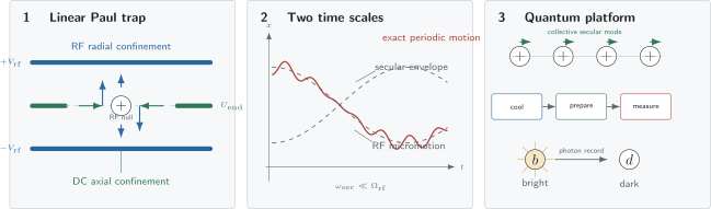
A linear Paul trap separates dynamical radial confinement from static axial confinement. Within the first Mathieu stability region, the exact periodic trajectory can be decomposed approximately into slow secular motion and an RF modulation. Laser cooling prepares quantized secular modes; internal bright–dark states are then inferred from a calibrated fluorescence record.

Secular Motion and the Pseudopotential

Small-parameter solution

For $|a_x|\ll1$ and $q_x^2\ll1$, the characteristic exponent is

$$\beta_x \simeq \sqrt{a_x+\frac{q_x^2}{2}},$$

so the slow secular angular frequency is

$$\omega_x \simeq \frac{\Omega_{\mathrm{rf}}}{2} \sqrt{a_x+\frac{q_x^2}{2}}.$$

To first order in $q_x$, a representative trajectory is

$$x(t) \simeq X\cos(\omega_xt+\varphi) \left[ 1-\frac{q_x}{2} \cos(\Omega_{\mathrm{rf}}t) \right].$$

This expression displays two time scales:

• $X\cos(\omega_xt+\varphi)$ is the slow secular motion;
• the factor oscillating at $\Omega_{\mathrm{rf}}$ is micromotion.

The sign of the modulation depends on the RF phase convention. Its magnitude relative to the secular displacement is $|q_x|/2$ at this order.

Effective potential energy

Let $\mathbf E_{\mathrm{rf}}(\mathbf r)$ be the amplitude of the RF electric field, so that the rapidly oscillating field is $\mathbf E_{\mathrm{rf}}(\mathbf r)\cos\Omega_{\mathrm{rf}}t$. Averaging over the fast motion gives the ponderomotive or pseudopotential energy

$$U_{\mathrm{ps}}(\mathbf r) = \frac{Q^2} {4m\Omega_{\mathrm{rf}}^2} \left| \mathbf E_{\mathrm{rf}}(\mathbf r) \right|^2.$$

For the ideal quadrupole,

$$U_{\mathrm{ps}}(x,y) = \frac{Q^2V_{\mathrm{rf}}^2} {4m\Omega_{\mathrm{rf}}^2r_0^4} \left(x^2+y^2\right).$$

Matching this to

$$U_{\mathrm{ps}} = \frac{m\omega_{\mathrm{rf}}^2}{2} \left(x^2+y^2\right)$$

gives

$$\omega_{\mathrm{rf}} = \frac{|Q|V_{\mathrm{rf}}} {\sqrt{2}\,m\Omega_{\mathrm{rf}}r_0^2} = \frac{|q|\Omega_{\mathrm{rf}}} {2\sqrt{2}}$$

when $a=0$.

The effective confinement becomes weaker when the drive frequency is increased at fixed voltage, because the ion has less time to acquire the correlated fast displacement that produces the average restoring force. Holding $q$ fixed while increasing $\Omega_{\mathrm{rf}}$, however, requires $V_{\mathrm{rf}}\propto\Omega_{\mathrm{rf}}^2$ and increases the secular frequency. Statements about scaling must say which control variable is held fixed.

Domain of validity

The pseudopotential is reliable when:

1. $|q|$ and $|a|$ are sufficiently small;
2. secular amplitudes remain in the nearly quadrupolar region;
3. the secular spectrum is well separated from the RF drive and dangerous nonlinear resonances;
4. applied forces vary slowly compared with $\Omega_{\mathrm{rf}}$;
5. micromotion-sensitive observables are either averaged correctly or modeled with the full periodic dynamics.

It can fail near stability boundaries, in strongly anharmonic electrode fields, during rapid transport, for large Coulomb crystals, or when laser coupling resolves RF sidebands. The effective potential predicts secular confinement; it does not erase the periodic kinetic energy.

Micromotion

Intrinsic micromotion

Intrinsic micromotion is the RF modulation tied to secular displacement. In the lowest-order solution,

$$x_{\mathrm{imm}}(t) \simeq - \frac{q_x}{2} x_{\mathrm{sec}}(t) \cos(\Omega_{\mathrm{rf}}t).$$

Cooling the secular oscillator toward its ground state reduces the spatial extent sampled by this term, but the exact trapped state remains a Floquet state with periodic motion. It is therefore imprecise to say that ground-state cooling removes all micromotion.

Excess micromotion from a displaced equilibrium

A static stray field $E_s$ displaces an ion from the RF null. In one harmonic direction,

$$x_d = \frac{QE_s} {m\omega_x^2}.$$

The corresponding first-order excess-micromotion amplitude is

$$x_{\mathrm{emm}} \simeq \frac{|q_x|}{2}|x_d|.$$

This motion persists even if the secular state has $\bar n\ll1$. It can produce:

• first-order Doppler modulation and RF sidebands;
• second-order Doppler shifts;
• RF AC Stark shifts;
• altered laser-cooling forces;
• collision energy that cannot be represented by a secular temperature;
• gate and spectroscopy errors.

Compensation electrodes apply static fields that move the equilibrium back toward the RF null. A complete three-dimensional compensation also addresses RF phase imbalance between electrodes, which can create driven motion along a nominally field-free axis.

Detecting and compensating micromotion

Three established diagnostics probe different projections and systematics:

Diagnostic	Observable	Important caveat
position versus confinement strength	displacement changes as the secular frequency is varied	requires calibrated imaging and distinguishes static-force directions
resolved RF sidebands	modulation index on a narrow optical transition	optical phase and AC Stark modulation can contribute
photon correlation	fluorescence modulation relative to the RF phase	depends on cooling-transition detuning, saturation, and laser direction

No single laser beam is sensitive to motion perpendicular to its wavevector. Micromotion should be bounded along enough independent directions, under the same voltages used for the experiment, and rechecked after loading or charging events. Berkeland et al. give the classic quantitative treatment of these methods.

Linear Paul Traps

A linear Paul trap uses an approximately two-dimensional RF quadrupole for radial confinement and static end electrodes for axial confinement. Near the center, write the endcap potential as

$$\Phi_{\mathrm{end}} \simeq \frac{\kappa U_{\mathrm{end}}}{z_0^2} \left[ z^2-\frac{x^2+y^2}{2} \right],$$

where $\kappa$ is a dimensionless geometry factor. The axial frequency is

$$\omega_z^2 = \frac{2Q\kappa U_{\mathrm{end}}} {mz_0^2}.$$

Laplace’s equation forces the accompanying radial curvature to be defocusing. In an ideal symmetric trap,

$$\omega_x^2 \simeq \omega_{\mathrm{rf}}^2 - \frac{\omega_z^2}{2}, \qquad \omega_y^2 \simeq \omega_{\mathrm{rf}}^2 - \frac{\omega_z^2}{2}.$$

Additional DC quadrupoles intentionally split $\omega_x$ and $\omega_y$ or rotate the radial principal axes. The sum of the three static electric curvatures must still vanish. Thus axial confinement is not an independent addition to the radial problem: it spends part of the radial stability margin.

Practical trap geometries include:

• three-dimensional ring-and-endcap traps;
• four-rod linear traps;
• segmented linear traps for axial shaping and ion transport;
• surface-electrode traps fabricated in one plane;
• cryogenic traps used to reduce some noise and vacuum limitations.

The ideal Mathieu model remains the organizing approximation, but numerical electrostatics is normally required to convert electrode voltages into curvatures, RF fields, anharmonicities, and transport waveforms.

Quantized Secular Motion

One ion

Near a stable equilibrium, the secular Hamiltonian is

$$H_{\mathrm{mot}} = \sum_{\alpha=x,y,z} \hbar\omega_\alpha \left( a_\alpha^\dagger a_\alpha+\frac{1}{2} \right).$$

For one mode,

$$x = x_0(a+a^\dagger), \qquad x_0 = \sqrt{\frac{\hbar}{2m\omega}}.$$

The oscillator quantum number $n$ refers to the secular mode in the effective description. The exact periodically driven quantum state has RF-periodic micromotion dressing. This distinction matters when comparing oscillator tomography, Doppler shifts, and full time-resolved trajectories.

A laser with wavevector projection $k_{\mathrm{eff}}$ couples to motion through

$$e^{ik_{\mathrm{eff}}x} = \exp\!\left[ i\eta(a+a^\dagger) \right], \qquad \eta=k_{\mathrm{eff}}x_0.$$

The Lamb–Dicke condition

$$\eta\sqrt{2\bar n+1}\ll1$$

means that the optical phase changes little across the occupied wavepacket. It is a condition on mode, beam geometry, and motional state, not a universal property of an ion species.

Trap depth is not an oscillator frequency

The local curvature determines $\omega$, whereas escape is controlled by the global time-dependent electrode potential, nonlinear resonances, collisions, and finite electrode apertures. A harmonic fit alone cannot establish trap depth. Conversely, a large nominal pseudopotential depth does not ensure low heating or good optical control.

Coulomb Crystals and Motional Modes

For $N$ equal ions in a harmonic secular potential, a useful effective potential energy is

$$\begin{aligned} U &= \sum_{i=1}^{N} \frac{m}{2} \left( \omega_x^2x_i^2 + \omega_y^2y_i^2 + \omega_z^2z_i^2 \right) \\ &\quad + \sum_{i<j} \frac{Q^2} {4\pi\epsilon_0 |\mathbf r_i-\mathbf r_j|}. \end{aligned}$$

At sufficiently low secular temperature, the ions localize near equilibrium positions that minimize $U$. The term Coulomb crystal describes this ordered configuration; it does not imply electronic crystalline bonding.

Linear chains

When radial confinement is much stronger than axial confinement, the equilibrium positions form a chain along the RF null. If radial confinement is reduced, a transverse normal-mode frequency softens and the chain can undergo a zigzag structural transition. Large crystals can sample anharmonicity and RF fields away from the null, so the single-particle pseudopotential test must be repeated for the many-ion configuration.

Normal-mode construction

Let $u_{i\alpha}$ be a small displacement from equilibrium. Expand to second order:

$$U \simeq U_0 + \frac{1}{2} \sum_{i\alpha,j\beta} K_{i\alpha,j\beta} u_{i\alpha}u_{j\beta},$$

where

$$K_{i\alpha,j\beta} = \left. \frac{\partial^2U} {\partial u_{i\alpha}\partial u_{j\beta}} \right|_{\mathrm{eq}}.$$

For equal masses, diagonalizing $K/m$ gives eigenvalues $\omega_m^2$ and orthonormal eigenvectors $b_{i\alpha,m}$. Quantization gives

$$u_{i\alpha} = \sum_m b_{i\alpha,m} \sqrt{\frac{\hbar}{2m\omega_m}} \left(a_m+a_m^\dagger\right).$$

Each laser couples to a mode with a participation factor $\mathbf k_{\mathrm{eff}}\cdot\mathbf b_{i,m}$. A mode can be cold yet nearly invisible to a poorly oriented probe, or strongly driven by spatially correlated electric-field noise. Quoting one “ion temperature” can hide this mode dependence.

Two-ion benchmark

For two equal ions at $z=\pm z_e$, force balance gives

$$z_e^3 = \frac{Q^2} {16\pi\epsilon_0m\omega_z^2}.$$

The axial center-of-mass and stretch frequencies are

$$\omega_{\mathrm{COM}}=\omega_z, \qquad \omega_{\mathrm{str}}=\sqrt{3}\,\omega_z.$$

These values are a useful calibration benchmark. Significant disagreement can signal unequal masses, anharmonic confinement, incorrect frequency assignment, or a geometry outside the assumed one-dimensional equilibrium.

Internal States

Confinement acts on the ion’s center of mass, while spectroscopy and quantum control usually use electronic, fine-structure, hyperfine, or Zeeman states. The mapping from an atomic spectrum to an effective two-level system is an engineering choice.

Encoding	Typical control	Strengths	Leading qualifications
optical qubit	narrow electric-quadrupole or octupole transition	direct optical addressing; useful for clocks and coherent control	laser coherence, finite excited-state lifetime, off-resonant levels
hyperfine clock qubit	microwaves or stimulated Raman fields	long coherence near field-insensitive points	Raman scattering, differential light shifts, extra repumping levels
Zeeman qubit	RF, microwave, or Raman fields	simple level structure and control	first-order magnetic-field sensitivity unless protected
metastable shelving state	optical excitation and fluorescence mapping	large bright–dark contrast	spontaneous decay and imperfect state transfer

Common species include $^9\mathrm{Be}^+$, $^{25}\mathrm{Mg}^+$, $^{40}\mathrm{Ca}^+$, $^{88}\mathrm{Sr}^+$, $^{138}\mathrm{Ba}^+$, and ytterbium isotopes. Species choice determines wavelengths, level complexity, branching ratios, isotope structure, clock transitions, and available photoionization paths. It does not by itself determine coherence or measurement fidelity; the magnetic environment, lasers, collection optics, and control protocol remain part of the system.

Hyperfine Structure, The Zeeman Effect in Atoms, and Atomic Selection Rules provide the atomic-structure background.

Loading and Initial Preparation

A typical preparation sequence is:

1. produce neutral atoms from an oven, ablation source, or atomic beam;
2. ionize the desired isotope, preferably with isotope-selective photoionization;
3. capture the ion within the trap’s stable phase-space region;
4. Doppler cool and detect fluorescence;
5. compensate static fields and characterize micromotion;
6. optically pump the internal state;
7. cool selected secular modes further if the protocol requires it.

Electron-impact ionization can load many species but often adds charging, background gas, and poor isotope selectivity. Resonant photoionization offers more control but can still charge exposed dielectrics. Loading therefore changes the trap environment and may invalidate a previously measured micromotion compensation.

Background-gas collisions can reorder a mixed-species chain, transfer motional energy, cause chemical reactions, or eject an ion. A long storage lifetime is evidence about rare loss processes; it is not a direct measurement of the low-frequency electric-field noise that controls motional heating.

Cooling the Secular Modes

Doppler cooling

Radiation pressure from red-detuned light provides velocity-dependent damping while spontaneous emission supplies momentum diffusion. In the ideal low-saturation two-level limit, the familiar minimum temperature is

$$k_BT_D = \frac{\hbar\Gamma}{2},$$

where $\Gamma$ is the excited-state population decay rate in angular-frequency units. Real ions require repump lasers, polarization control, magnetic fields, and treatment of multilevel dark states. The ideal formula is therefore a scale, not a universal thermometer.

For a thermal oscillator,

$$\bar n = \frac{1} {\exp(\hbar\omega/k_BT)-1}.$$

When $k_BT\gg\hbar\omega$,

$$\bar n \simeq \frac{k_BT}{\hbar\omega}.$$

Because typical optical linewidths can greatly exceed secular frequencies, Doppler cooling often leaves $\bar n\gg1$ even though the ion is localized on a microscopic scale.

Resolved-sideband cooling

If motional sidebands are spectrally resolved,

$$\omega_m\gg\Gamma_{\mathrm{eff}},$$

one can drive a red sideband

$$|g,n\rangle \longrightarrow |e,n-1\rangle$$

and use dissipative repumping to return the internal state while usually preserving the reduced motional number in the Lamb–Dicke regime. Repetition accumulates population near $n=0$, where the red sideband vanishes.

Ground-state cooling was demonstrated in one dimension by Diedrich et al. and in all three dimensions with Raman sideband cooling by Monroe et al. The present platform page uses those results as evidence that the oscillator description is experimentally addressable; detailed cooling-rate derivations belong to the cooling pages.

Other cooling strategies

• EIT cooling can cool multiple modes over a broader engineered spectral window than a single narrow red sideband.
• Sympathetic cooling uses a second ion species to remove motion without directly scattering photons from a protected spectroscopy or logic ion.
• Continuous cooling can stabilize spectator modes but may introduce scattering and differential forces during coherent operations.

Cooling is mode specific. A reported $\bar n$ should identify the mode, diagnostic, fit model, and delay between cooling and use.

Measuring Internal and Motional States

State-dependent fluorescence

The standard internal-state measurement maps one state to a nearly closed cycling transition and leaves another state dark or shelved. During a detection interval, the apparatus records a photon count $n$ or a time-resolved sequence of counts.

In the simplest static model,

$$\begin{aligned} P(n|b) &= e^{-\mu_b} \frac{\mu_b^n}{n!}, \\ P(n|d) &= e^{-\mu_d} \frac{\mu_d^n}{n!}, \end{aligned}$$

with $\mu_b\gg\mu_d$. A threshold or likelihood-ratio rule classifies the state. This model must be enlarged when the dark state decays, off-resonant pumping changes the state during detection, the collection rate drifts, or neighboring ions overlap on a camera.

Electron shelving made individual quantum jumps directly visible as bright and dark fluorescence intervals. Modern time-resolved likelihood methods can outperform a fixed count threshold because the timing of photons helps distinguish a genuinely bright state from a dark state that decays partway through detection.

The canonical open-system and trajectory interpretation is given in Trapped Ions and Quantum-Jump Trajectories.

Motional diagnostics

Common diagnostics include:

• secular-frequency spectroscopy with a weak electric or optical drive;
• red-to-blue sideband asymmetry near the ground state;
• Rabi oscillations whose $n$-dependent frequencies reveal a number distribution;
• controlled displacement followed by internal-state mapping;
• imaging of equilibrium positions and thermally broadened spatial distributions;
• heating-rate measurements after a variable delay without cooling.

For an ideal thermal mode in the Lamb–Dicke and weak-excitation limits, integrated first-sideband strengths obey

$$\frac{I_{\mathrm{red}}} {I_{\mathrm{blue}}} = \frac{\bar n} {\bar n+1}.$$

This is a self-calibrating thermometer only within its assumptions. Probe saturation, off-resonant carrier excitation, nonthermal distributions, micromotion sidebands, mode overlap, and state-preparation error can bias the inferred $\bar n$.

Heating and Environmental Coupling

For a single mode polarized along unit vector $\mathbf e_m$, electric-field noise near $\omega_m$ drives transitions between oscillator levels. With one common one-sided spectral-density convention,

$$\dot{\bar n}_m = \frac{Q^2} {4m\hbar\omega_m} S_{E,m}(\omega_m).$$

The numerical prefactor changes with one-sided versus two-sided and angular- frequency versus ordinary-frequency conventions. A heating-rate result should therefore report the convention before converting to $S_E$.

Technical pickup, electrode-voltage noise, dielectric charging, fluctuating surface potentials, RF noise near secular sidebands, and collisions can all contribute. The extensive evidence and open questions concerning surface-related electric-field noise belong to the open-system trapped-ion page and the review by Brownnutt et al.

Worked Scale Audit: One Calcium Ion

Consider an idealized $^{40}\mathrm{Ca}^+$ ion with

$$\begin{gathered} Q=e, \qquad m=39.9626\,u, \\ r_0=0.500\ \mathrm{mm}, \qquad V_{\mathrm{rf}}=200\ \mathrm{V}, \\ \frac{\Omega_{\mathrm{rf}}}{2\pi} = 20.0\ \mathrm{MHz}, \qquad U_{\mathrm{dc}}=0. \end{gathered}$$

Here $V_{\mathrm{rf}}$ is the zero-to-peak voltage in the ideal quadrupole potential. The Mathieu parameter is

$$q = \frac{2eV_{\mathrm{rf}}} {mr_0^2\Omega_{\mathrm{rf}}^2} = 0.2446.$$

The RF-only secular frequency is

$$\frac{\omega_{\mathrm{rf}}}{2\pi} = \frac{q\Omega_{\mathrm{rf}}} {4\sqrt{2}\,\pi} = 1.730\ \mathrm{MHz}.$$

The associated zero-point length is

$$x_0 = \sqrt{\frac{\hbar}{2m\omega_{\mathrm{rf}}}} = 8.55\ \mathrm{nm}.$$

If static end electrodes produce $\omega_z/(2\pi)=0.500\ \mathrm{MHz}$, the ideal radial defocusing estimate gives

$$\frac{\omega_r}{2\pi} \simeq \frac{1}{2\pi} \sqrt{ \omega_{\mathrm{rf}}^2-\frac{\omega_z^2}{2} } = 1.693\ \mathrm{MHz}.$$

Now suppose a transverse static stray field is $E_s=10.0\ \mathrm{V\,m^{-1}}$. Using the RF-only curvature for a transparent scale estimate,

$$x_d = \frac{eE_s} {m\omega_{\mathrm{rf}}^2} = 204\ \mathrm{nm},$$

and

$$x_{\mathrm{emm}} \simeq \frac{q}{2}x_d = 25.0\ \mathrm{nm}.$$

The excess-micromotion amplitude is about three times the secular zero-point length despite the apparently modest static field. This comparison explains why micromotion compensation is a precision calibration, not merely a visual centering step.

These numbers are not predictions for a particular electrode structure. Replacing the ideal quadrupole by a real trap requires geometry factors from electrostatic modeling, measured secular frequencies, RF-voltage calibration, and a check for phase-driven micromotion.

Calibration and Validation Ladder

A credible trapped-ion platform claim should move through several layers of evidence.

1. Electrical and geometric model

Document:

• electrode geometry and coordinate convention;
• voltage amplitudes, offsets, phases, and RF frequency;
• filters, resonator response, and electrode transfer functions;
• simulated basis potentials and the mesh or convergence test;
• expected quadrupole curvature and leading anharmonic terms.

2. Stable confinement

Measure:

• secular frequencies and principal-axis orientations;
• stability margin under voltage variation;
• equilibrium positions and ion order;
• storage and collision statistics;
• dependence on ion number and species.

Agreement between one measured frequency and an ideal formula does not validate the global potential.

3. Micromotion

Bound:

• static-field displacement along independent directions;
• RF-correlated fluorescence or resolved RF sidebands;
• phase-imbalance-driven motion;
• variation after loading, transport, and dielectric illumination.

The relevant bound is set by the observable: a quantum gate, collision experiment, and optical clock can require different projections and sensitivities.

4. Motional preparation

Report:

• $\bar n_m$ or a fuller distribution for each relevant mode;
• the thermometry model and probe regime;
• heating rates and delays between cooling and operation;
• mode-frequency drift and avoided crossings;
• evidence that spectator modes do not invalidate the model.

5. Internal preparation and measurement

Characterize:

• optical-pumping leakage;
• bright and dark count distributions;
• state changes during the detection interval;
• detector dead time, background, and spatial crosstalk;
• calibration drift and uncertainty propagation.

Preparation and measurement errors should be separated when possible. A single observed bright fraction combines both unless independently constrained.

6. Task-level validation

Finally, test the actual operation under the same trap settings, laser powers, timing, ion number, and analysis pipeline used for the claimed result. A beautiful micromotion scan performed under different voltages is supporting evidence, not a substitute for task-level validation.

Model and Error Ledger

Layer	Working model	Leading failure modes	Direct checks
RF confinement	ideal Mathieu equation	geometry factors, higher multipoles, RF imbalance	boundary-element or finite-element model; stability scan
secular dynamics	harmonic pseudopotential	large $q$, anharmonicity, nonlinear resonances	frequency versus amplitude and voltage
ion crystal	quadratic normal modes	structural transition, mode mixing, unequal masses	imaging and mode spectroscopy
cooling	thermal or near-ground-state mode	dark states, recoil, unresolved modes, nonthermal tails	sideband asymmetry and Rabi data
fluorescence	fixed bright/dark count models	pumping and decay during readout, crosstalk	time-tagged calibration records
heating	stationary electric-field noise	drift, bursts, collisions, nonstationarity	delay scans over multiple times and days

The point of the ledger is not to demand every possible measurement. It is to match the validation burden to the approximation on which the scientific claim depends.

Common Mistakes

Calling the pseudopotential the electric potential

The pseudopotential is an averaged effective energy proportional to $|\mathbf E_{\mathrm{rf}}|^2$. The instantaneous electric potential remains a sign-changing quadrupole.

Mixing voltage conventions

A zero-to-peak amplitude $V_{\mathrm{rf}}$, an RMS voltage $V_{\mathrm{rf}}/\sqrt{2}$, and a peak-to-peak voltage $2V_{\mathrm{rf}}$ produce different numerical $q$ values if substituted without conversion.

Replacing angular frequency by ordinary frequency

The Mathieu parameter contains $\Omega_{\mathrm{rf}}^2$, not $f_{\mathrm{rf}}^2$. Omitting $2\pi$ changes $q$ by $4\pi^2$.

Treating stability as instantaneous focusing

The trap is stable because the periodic equation has bounded Floquet solutions. At each instant, one quadrupole direction is defocusing.

Equating secular ground-state cooling with zero motion

The secular ground state has zero-point fluctuations, and Paul-trap states retain periodic micromotion dressing. Excess micromotion is a separate calibration.

Assigning one temperature to every mode

Normal modes have different frequencies, cooling couplings, heating rates, and occupations. A scalar temperature is justified only after establishing an appropriate thermal distribution.

Inferring state-readout fidelity from histogram separation alone

State changes during detection can produce errors even when static Poisson histograms barely overlap. Time-resolved records and independently prepared states are needed for a defensible model.

Using ion lifetime as a heating-rate measurement

Loss probes rare excursions out of the trapping region. Motional heating probes noise near a secular frequency. The two observables constrain different parts of the environment.

Exercises

Exercise 1: Derive the Mathieu parameters

Starting from

$$\Phi(x,y,t) = \frac{U_{\mathrm{dc}}-V_{\mathrm{rf}}\cos\Omega_{\mathrm{rf}}t} {2r_0^2} (x^2-y^2),$$

derive the Mathieu equations for $x$ and $y$. Explain why the signs of both $a$ and $q$ reverse between the two directions.

Solution

The fields are

$$E_x = - \frac{U_{\mathrm{dc}}-V_{\mathrm{rf}}\cos\Omega_{\mathrm{rf}}t} {r_0^2}x,$$

and

$$E_y = + \frac{U_{\mathrm{dc}}-V_{\mathrm{rf}}\cos\Omega_{\mathrm{rf}}t} {r_0^2}y.$$

Using $m\ddot{x}=QE_x$ gives

$$m\ddot{x} + \frac{Q}{r_0^2} \left( U_{\mathrm{dc}} - V_{\mathrm{rf}}\cos\Omega_{\mathrm{rf}}t \right)x =0.$$

Set $\tau=\Omega_{\mathrm{rf}}t/2$, so $d^2/dt^2=(\Omega_{\mathrm{rf}}^2/4)d^2/d\tau^2$. Then

$$\frac{d^2x}{d\tau^2} + \left[ \frac{4QU_{\mathrm{dc}}} {mr_0^2\Omega_{\mathrm{rf}}^2} - \frac{4QV_{\mathrm{rf}}} {mr_0^2\Omega_{\mathrm{rf}}^2} \cos2\tau \right]x =0.$$

Comparison with $x''+(a_x-2q_x\cos2\tau)x=0$ gives

$$a_x = \frac{4QU_{\mathrm{dc}}} {mr_0^2\Omega_{\mathrm{rf}}^2}, \qquad q_x = \frac{2QV_{\mathrm{rf}}} {mr_0^2\Omega_{\mathrm{rf}}^2}.$$

Because $\Phi$ contains $-y^2$ where it contains $+x^2$, the force curvature changes sign:

$$a_y=-a_x, \qquad q_y=-q_x.$$

This is the mathematical statement that the instantaneous quadrupole focuses one transverse direction while defocusing the other.

Exercise 2: Recover the pseudopotential frequency

For the ideal quadrupole with $U_{\mathrm{dc}}=0$, show that the pseudopotential gives

$$\omega_{\mathrm{rf}} = \frac{|q|\Omega_{\mathrm{rf}}}{2\sqrt{2}}.$$

Why does $\omega_{\mathrm{rf}}$ decrease with increasing $\Omega_{\mathrm{rf}}$ if $V_{\mathrm{rf}}$ is held fixed?

Solution

The RF-field amplitude is

$$\mathbf E_{\mathrm{rf}} = \frac{V_{\mathrm{rf}}}{r_0^2} (-x\,\mathbf e_x+y\,\mathbf e_y),$$

so

$$|\mathbf E_{\mathrm{rf}}|^2 = \frac{V_{\mathrm{rf}}^2}{r_0^4} (x^2+y^2).$$

The pseudopotential energy is

$$U_{\mathrm{ps}} = \frac{Q^2V_{\mathrm{rf}}^2} {4m\Omega_{\mathrm{rf}}^2r_0^4} (x^2+y^2).$$

Equating its coefficient to $m\omega_{\mathrm{rf}}^2/2$ gives

$$\omega_{\mathrm{rf}} = \frac{|Q|V_{\mathrm{rf}}} {\sqrt{2}\,m\Omega_{\mathrm{rf}}r_0^2}.$$

Since

$$|q| = \frac{2|Q|V_{\mathrm{rf}}} {mr_0^2\Omega_{\mathrm{rf}}^2},$$

substitution yields

$$\omega_{\mathrm{rf}} = \frac{|q|\Omega_{\mathrm{rf}}}{2\sqrt{2}}.$$

At fixed $V_{\mathrm{rf}}$, the fast displacement induced during one RF cycle decreases as the drive becomes faster, so the averaged restoring energy scales as $\Omega_{\mathrm{rf}}^{-2}$ and the frequency as $\Omega_{\mathrm{rf}}^{-1}$. At fixed $q$, by contrast, $V_{\mathrm{rf}}\propto\Omega_{\mathrm{rf}}^2$ and $\omega_{\mathrm{rf}}\propto\Omega_{\mathrm{rf}}$.

Exercise 3: Audit a calcium-ion trap

Use the parameters in the worked example to calculate $q$, $\omega_{\mathrm{rf}}/(2\pi)$, and $x_0$. Then repeat the $q$ calculation if the quoted $200\ \mathrm{V}$ were mistakenly interpreted as zero-to-peak when it was actually peak-to-peak.

Solution

With

$$\begin{gathered} m=39.9626\,u, \quad r_0=5.00\times10^{-4}\ \mathrm{m}, \\ \Omega_{\mathrm{rf}} = 2\pi(20.0\times10^6)\ \mathrm{s^{-1}}, \quad V_{\mathrm{rf}}=200\ \mathrm{V}, \end{gathered}$$

one finds

$$q = \frac{2eV_{\mathrm{rf}}} {mr_0^2\Omega_{\mathrm{rf}}^2} = 0.2446.$$

Then

$$\frac{\omega_{\mathrm{rf}}}{2\pi} = \frac{q}{2\sqrt{2}} \frac{\Omega_{\mathrm{rf}}}{2\pi} = 1.730\ \mathrm{MHz},$$

and

$$x_0 = \sqrt{\frac{\hbar}{2m\omega_{\mathrm{rf}}}} = 8.55\ \mathrm{nm}.$$

If $200\ \mathrm{V}$ is peak to peak, the zero-to-peak amplitude is only $100\ \mathrm{V}$. Because $q$ is linear in voltage,

$$q=0.1223.$$

The small-$q$ secular frequency is also halved, and the zero-point length increases by $\sqrt{2}$. Voltage convention is therefore not metadata; it changes the inferred dynamics.

Exercise 4: Excess micromotion from a stray field

An ion with secular frequency $\omega_x$ experiences a static field $E_s$. Derive its displaced equilibrium and first-order excess-micromotion amplitude. If $\omega_x$ is doubled while $q$ and $E_s$ are held fixed, by what factor does the excess-micromotion amplitude change?

Solution

The slow effective force is

$$F_{\mathrm{eff}} = - m\omega_x^2x+QE_s.$$

Setting it to zero gives

$$x_d = \frac{QE_s}{m\omega_x^2}.$$

The small-$q$ Mathieu solution modulates a static displacement by a fractional amplitude $|q|/2$, so

$$x_{\mathrm{emm}} \simeq \frac{|q|}{2} \frac{|Q E_s|}{m\omega_x^2}.$$

At fixed $q$ and $E_s$, doubling $\omega_x$ reduces both $x_d$ and $x_{\mathrm{emm}}$ by a factor of four. In a real trap, changing $\omega_x$ may also change $q$, the principal axes, or the stray field, so the experimental scaling test must track those quantities.

Exercise 5: Two-ion equilibrium and normal modes

Two equal ions are confined to the $z$ axis by a harmonic potential of frequency $\omega_z$. Derive their equilibrium positions and the axial center-of-mass and stretch frequencies.

Solution

Let the ions sit at $z_1=z_e$ and $z_2=-z_e$. With $C=Q^2/(4\pi\epsilon_0)$, the potential is

$$U(z_e) = m\omega_z^2z_e^2 + \frac{C}{2z_e}.$$

Force balance gives

$$\frac{dU}{dz_e} = 2m\omega_z^2z_e - \frac{C}{2z_e^2} =0,$$

and hence

$$z_e^3 = \frac{C}{4m\omega_z^2} = \frac{Q^2} {16\pi\epsilon_0m\omega_z^2}.$$

For small displacements $u_1,u_2$, the axial Hessian is

$$K = m\omega_z^2 \begin{pmatrix} 2 & -1\\ -1 & 2 \end{pmatrix}.$$

The normalized eigenvectors are proportional to $(1,1)$ and $(1,-1)$, with eigenvalues $m\omega_z^2$ and $3m\omega_z^2$. Therefore

$$\omega_{\mathrm{COM}}=\omega_z, \qquad \omega_{\mathrm{str}}=\sqrt{3}\,\omega_z.$$

The Coulomb force does not change the center-of-mass frequency because a uniform translation leaves the separation unchanged.

Exercise 6: Why Doppler cooling need not reach the ground state

For a hypothetical two-level ion with $\Gamma/(2\pi)=21.6\ \mathrm{MHz}$, calculate the ideal Doppler temperature. Estimate the thermal occupations of secular modes at $1.70\ \mathrm{MHz}$ and $0.500\ \mathrm{MHz}$. Use the exact Bose–Einstein oscillator expression.

Solution

The ideal Doppler temperature is

$$T_D = \frac{\hbar\Gamma}{2k_B} = \frac{h(21.6\ \mathrm{MHz})}{2k_B} \simeq 5.18\times10^{-4}\ \mathrm{K}.$$

For a mode of ordinary frequency $f$,

$$\bar n = \frac{1} {\exp(hf/k_BT_D)-1}.$$

At $f=1.70\ \mathrm{MHz}$,

$$\frac{hf}{k_BT_D} \simeq 0.157, \qquad \bar n\simeq5.90.$$

At $f=0.500\ \mathrm{MHz}$,

$$\frac{hf}{k_BT_D} \simeq 0.0463, \qquad \bar n\simeq21.1.$$

Thus sub-millikelvin cooling can still leave many secular quanta. The result uses an ideal two-level Doppler limit; multilevel structure, polarization, micromotion, recoil, and laser parameters change the actual steady state.

Exercise 7: Sideband-asymmetry thermometry

A weak probe measures an integrated red-to-blue first-sideband ratio $R=0.120$. Assuming a thermal mode and the ideal Lamb–Dicke weak-probe relation, infer $\bar n$ and the ground-state population $P_0$. Name three effects that could invalidate the inference.

Solution

For a thermal mode,

$$R = \frac{\bar n}{\bar n+1}.$$

Solving gives

$$\bar n = \frac{R}{1-R} = \frac{0.120}{0.880} = 0.136.$$

The thermal number distribution is

$$P_n = \frac{\bar n^n}{(\bar n+1)^{n+1}},$$

so

$$P_0 = \frac{1}{1+\bar n} = 0.880.$$

Possible failures include probe saturation, off-resonant carrier excitation, overlapping modes, micromotion sidebands, a nonthermal number distribution, state-preparation error, unequal red and blue detection transfer functions, and heating during the scan. Sideband asymmetry is powerful because many coupling factors cancel, but only within the model that produces the ratio.

Exercise 8: Design a confinement-to-readout audit

An experiment reports a trapped-ion qubit with low motional excitation and high state-readout fidelity. Design a minimal evidence package that tests the claim without assuming the ideal trap and Poisson readout models are exact.

Solution

A defensible package would include at least:

1. electrical definition: electrode geometry, RF amplitude convention, drive frequency, DC voltages, and simulated basis fields;
2. confinement checks: measured secular frequencies and axes, their voltage scaling, ion equilibrium positions, and a stated stability margin;
3. micromotion bounds: at least two independent spatial projections, including a check for RF phase imbalance under the operating voltages;
4. motional evidence: sideband or Rabi data for every task-relevant mode, the inferred distribution or $\bar n_m$, probe-model residuals, and heating rates over the operation delay;
5. preparation calibration: independently prepared internal basis states and leakage estimates;
6. readout records: time-tagged bright and dark calibration data, a model that allows state changes during detection, cross-validation, and drift monitoring;
7. task-level repetition: the same measurements interleaved with the claimed operation, rather than only in a separate favorable configuration.

The package should propagate uncertainty from voltage, frequency, photon count, and model parameters to the final reported quantities. Disagreement between the ideal formula and direct calibration is not automatically a failure of the experiment; it is evidence that geometry, anharmonicity, nonstationarity, or the measurement model must be enlarged.

References

1. W. Paul, “Electromagnetic traps for charged and neutral particles,” Reviews of Modern Physics 62, 531–540 (1990), doi:10.1103/RevModPhys.62.531.
2. D. Leibfried, R. Blatt, C. Monroe, and D. Wineland, “Quantum dynamics of single trapped ions,” Reviews of Modern Physics 75, 281–324 (2003), doi:10.1103/RevModPhys.75.281.
3. D. J. Wineland, C. Monroe, W. M. Itano, D. Leibfried, B. E. King, and D. M. Meekhof, “Experimental issues in coherent quantum-state manipulation of trapped atomic ions,” Journal of Research of the National Institute of Standards and Technology 103, 259–328 (1998), doi:10.6028/jres.103.019.
4. D. J. Berkeland, J. D. Miller, J. C. Bergquist, W. M. Itano, and D. J. Wineland, “Minimization of ion micromotion in a Paul trap,” Journal of Applied Physics 83, 5025–5033 (1998), doi:10.1063/1.367318.
5. D. F. V. James, “Quantum dynamics of cold trapped ions with application to quantum computation,” Applied Physics B 66, 181–190 (1998), doi:10.1007/s003400050373.
6. F. Diedrich, J. C. Bergquist, W. M. Itano, and D. J. Wineland, “Laser cooling to the zero-point energy of motion,” Physical Review Letters 62, 403–406 (1989), doi:10.1103/PhysRevLett.62.403.
7. C. Monroe, D. M. Meekhof, B. E. King, S. R. Jefferts, W. M. Itano, D. J. Wineland, and P. Gould, “Resolved-sideband Raman cooling of a bound atom to the 3D zero-point energy,” Physical Review Letters 75, 4011–4014 (1995), doi:10.1103/PhysRevLett.75.4011.
8. D. J. Wineland and W. M. Itano, “Laser cooling of atoms,” Physical Review A 20, 1521–1540 (1979), doi:10.1103/PhysRevA.20.1521.
9. J. C. Bergquist, R. G. Hulet, W. M. Itano, and D. J. Wineland, “Observation of quantum jumps in a single atom,” Physical Review Letters 57, 1699–1702 (1986), doi:10.1103/PhysRevLett.57.1699.
10. A. H. Myerson et al., “High-fidelity readout of trapped-ion qubits,” Physical Review Letters 100, 200502 (2008), doi:10.1103/PhysRevLett.100.200502.
11. M. Brownnutt, M. Kumph, P. Rabl, and R. Blatt, “Ion-trap measurements of electric-field noise near surfaces,” Reviews of Modern Physics 87, 1419–1482 (2015), doi:10.1103/RevModPhys.87.1419.
12. H. Häffner, C. F. Roos, and R. Blatt, “Quantum computing with trapped ions,” Physics Reports 469, 155–203 (2008), doi:10.1016/j.physrep.2008.09.003.
13. C. D. Bruzewicz, J. Chiaverini, R. McConnell, and J. M. Sage, “Trapped-ion quantum computing: Progress and challenges,” Applied Physics Reviews 6, 021314 (2019), doi:10.1063/1.5088164.
14. D. Kielpinski, C. Monroe, and D. J. Wineland, “Architecture for a large-scale ion-trap quantum computer,” Nature 417, 709–711 (2002), doi:10.1038/nature00784.
15. L. S. Brown and G. Gabrielse, “Geonium theory: Physics of a single electron or ion in a Penning trap,” Reviews of Modern Physics 58, 233–311 (1986), doi:10.1103/RevModPhys.58.233.

Cross-Links

• Optical Clocks develops single-ion and quantum-logic clock architectures, micromotion and time-dilation shifts, quadrupole averaging, comb readout, and clock comparisons.
• AMO Platforms and Quantum Control places ion traps in the full preparation–control–measurement cycle.
• Laser Cooling and Radiation Pressure develop the force and diffusion physics used for initial cooling.
• Floquet Theory in Quantum Mechanics supplies the general language behind stable Mathieu solutions and micromotion dressing.
• Trapped Ions follows motional heating, fluorescence backaction, dephasing, and trajectories as open-system processes.
• Approximation Checklist helps audit the Markov, rotating-wave, harmonic, and effective-model assumptions used in later control analyses.