Magneto-Optical Traps

A magneto-optical trap, or MOT, combines red-detuned optical molasses with a magnetic-field gradient and polarization-selective transitions. The Doppler shift makes the force oppose velocity. The Zeeman shift makes the force oppose displacement. Near the trap center,

$$\mathbf F \simeq - \boldsymbol{\kappa}\mathbf r - \boldsymbol{\alpha}\mathbf v.$$

The first term confines; the second damps. Neither the light alone nor the quadrupole magnetic field alone generally provides the standard MOT force. The trap exists because displacement changes which counterpropagating beam is closer to resonance.

A MOT is an open, driven, dissipative system. It continually scatters photons, diffuses momentum, optically pumps internal states, loads atoms from an external source, and loses them through collisions. Its steady state is not simply thermal equilibrium in a conservative potential.

Canonical Scope

This page owns:

1. the one-dimensional Zeeman-plus-Doppler force;
2. the sign of the restoring force;
3. the three-dimensional quadrupole and beam geometry;
4. linear trap dynamics, size, and gravitational sag;
5. capture, loading, one-body loss, and two-body loss;
6. density limits, diagnostics, operating sequences, and common failures.

Doppler Cooling owns the optical-molasses friction and recoil-diffusion derivation. Radiation Pressure owns the single-beam scattering force. Zeeman Effect in Atoms owns the atomic level shifts and $g$-factor conventions. Sub-Doppler Cooling owns polarization-gradient and dark-state mechanisms that may coexist with, or be suppressed by, the MOT field.

Optical Dipole Traps owns conservative AC Stark confinement, Gaussian-beam frequencies, and the depth–scattering tradeoff. The MOT is the dissipative capture and precooling stage from which those traps are commonly loaded.

One-dimensional model

Conventions

Take two beams along $\pm x$, both with wave-number magnitude $k$. Use the chapter’s atom-minus-laser detuning:

$$\Delta = \omega_0-\omega_L.$$

Red detuning means $\Delta>0$. Let the local magnetic field be

$$B_x(x) = B'x.$$

The two beam helicities address transitions with opposite Zeeman shifts. Label the polarizations so that, for positive effective magnetic moment $\mu_{\mathrm{eff}}$,

$$\beta = \frac{\mu_{\mathrm{eff}}B'}{\hbar} > 0.$$

For velocity $v$ along $+x$, define the effective detunings

$$\begin{aligned} \Delta_+(x,v) &= \Delta + kv + \beta x, \\ \Delta_-(x,v) &= \Delta - kv - \beta x. \end{aligned}$$

The subscripts identify beam momentum $\pm\hbar k$. These equations already encode the chosen helicities. Reversing either the field gradient or both beam helicities reverses the sign of the position term.

Why the displaced atom is pushed inward

Set $v=0$ and place the atom at $x>0$. Then

$$\Delta_+ = \Delta+\beta x, \qquad \Delta_- = \Delta-\beta x.$$

For red detuning and small displacement, the $-x$ beam is closer to resonance:

$$|\Delta_-| < |\Delta_+|.$$

It therefore scatters more strongly and supplies momentum $-\hbar k$, toward the origin. At $x<0$, the roles reverse. The polarization assignment is correct only if this sign test succeeds.

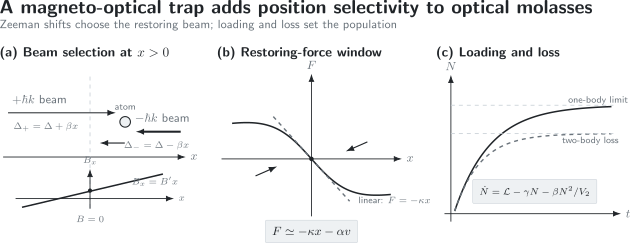
At $x>0$, the Zeeman shift moves the inward-propagating beam closer to resonance. The force is linear only near the origin and within the capture window. The trapped population is set separately by loading rate $\mathcal L$, one-body loss $\gamma$, and density-dependent two-body loss $\beta$.

Restoring-force derivation

Weak-saturation scattering rate

For a closed transition and independent weak beams, use

$$R(\delta) = \frac{\Gamma s}{2} \frac{1}{ 1+(2\delta/\Gamma)^2 }.$$

The net force is

$$F(x,v) = \hbar k \left[ R(\Delta_+) - R(\Delta_-) \right].$$

This compact expression contains both trapping and damping. It remains a two-level model: real MOTs require multilevel optical pumping, repumping, beam saturation, and a position-dependent quantization axis.

Linear expansion

Define

$$q = kv+\beta x.$$

Near $x=v=0$,

$$R(\Delta\pm q) \simeq R(\Delta) \pm qR'(\Delta).$$

Therefore

$$\begin{aligned} F(x,v) &\simeq 2\hbar kR'(\Delta) \left( kv+\beta x \right) \\ &= -\alpha v-\kappa x, \end{aligned}$$

with

$$\alpha = -2\hbar k^2R'(\Delta),$$

and

$$\kappa = -2\hbar k\beta R'(\Delta).$$

For

$$D = 1+\left(\frac{2\Delta}{\Gamma}\right)^2,$$

the derivative is

$$R'(\Delta) = - \frac{ 4s(\Delta/\Gamma) }{ D^2 }.$$

Hence

$$\alpha = 8\hbar k^2s \frac{ \Delta/\Gamma }{ D^2 },$$

and

$$\kappa = 8\hbar k\beta s \frac{ \Delta/\Gamma }{ D^2 }.$$

For $\Delta>0$ and $\beta>0$, both coefficients are positive. A useful consistency relation is

$$\frac{\kappa}{\alpha} = \frac{\beta}{k} = \frac{ \mu_{\mathrm{eff}}B' }{ \hbar k }.$$

The same spectral slope sets damping and confinement; the field gradient converts displacement into an effective Doppler shift.

Saturation and shared excited-state population

At higher intensity, one often replaces the denominator by

$$1+s_{\mathrm{tot}} + \left( \frac{2\delta}{\Gamma} \right)^2.$$

This is only a representative correction. Counterpropagating beams share the same excited-state population, while multilevel Clebsch–Gordan coefficients and optical pumping make the saturation state dependent. A quantitative MOT model generally solves position- and velocity-dependent optical Bloch or rate equations.

Three-dimensional geometry

Quadrupole field

An anti-Helmholtz coil pair creates a field zero near the trap center. If $B'$ denotes the axial gradient, an ideal local field is

$$\mathbf B(\mathbf r) = B' \left( \frac{x}{2}\hat{\mathbf x} + \frac{y}{2}\hat{\mathbf y} - z\hat{\mathbf z} \right).$$

The factors are required by

$$\boldsymbol{\nabla}\cdot\mathbf B = 0.$$

The radial gradient is half the axial magnitude. Consequently, equal beam parameters do not imply equal spring constants in all directions.

Six-beam configuration

The conventional three-dimensional MOT uses one counterpropagating beam pair along each Cartesian axis. Relative helicities are chosen so that the beam propagating toward the field zero addresses the locally favored transition.

The labels $\sigma^+$ and $\sigma^-$ are defined relative to a quantization axis, not merely by a laboratory drawing of circular polarization. Because the quadrupole field changes direction through the cloud, a correct sign argument must track:

1. beam propagation direction;
2. local magnetic-field direction;
3. the addressed $\Delta m_F=\pm1$ transition;
4. the transition’s effective Zeeman shift.

Near the exact field zero, the quantization axis is not well defined. The simple independent-axis picture is then qualitative; full multilevel dynamics determines optical pumping and dark-state structure.

Alternative optical layouts

Mirror MOTs, pyramidal MOTs, and grating MOTs generate the required beam directions with reflections or diffraction. Two-dimensional MOTs cool and collimate an atomic beam while allowing longitudinal flux. Narrow-line MOTs use a small $\Gamma$, so gravity, recoil, and field curvature become more prominent. Molecular and blue-detuned MOTs can require type-II transitions, polarization or magnetic remixing, and force mechanisms beyond the simple two-level type-I model.

The local test remains the same: calculate the actual transition shifts and show that displacement increases inward scattering.

Linear trap dynamics

Damped oscillator

Along one principal axis,

$$m\ddot x + \alpha\dot x + \kappa x = 0.$$

Define

$$\omega_0 = \sqrt{\frac{\kappa}{m}}, \qquad \Gamma_m = \frac{\alpha}{2m}.$$

The characteristic exponents are

$$r_\pm = -\Gamma_m \pm \sqrt{ \Gamma_m^2-\omega_0^2 }.$$

The motion is underdamped when $\Gamma_m<\omega_0$, critically damped when they are equal, and overdamped when $\Gamma_m>\omega_0$. Many broad-line MOTs are strongly damped, so a displaced cloud may return without visible oscillation.

The measured relaxation rates need not equal this two-level prediction. Sub-Doppler forces, beam imbalance, multiple scattering, changing cloud size, and internal-state delays alter them.

Local effective potential

The position part of the linear force can be represented by

$$U_{\mathrm{eff}}(x) = \frac{1}{2}\kappa x^2.$$

This is a local pseudopotential, useful for cloud-size and sag estimates. The full MOT force is dissipative, velocity dependent, saturating, and generally not derivable from a global scalar potential.

Cloud size

If one principal direction is approximately harmonic and the motional distribution is thermal,

$$n(x) \propto \exp \left( - \frac{\kappa x^2}{2k_{\mathrm B}T} \right).$$

The rms width is

$$\sigma_x = \sqrt{ \frac{k_{\mathrm B}T}{\kappa} }.$$

This relation can infer $\kappa$ from an independently measured temperature and cloud width. It fails in a density-limited, non-Gaussian, anisotropic, or strongly multiple-scattering cloud.

Gravity and constant forces

Along vertical coordinate $z$, add gravity:

$$F_z = -\kappa_z z-\alpha_z v_z-mg.$$

The equilibrium sag is

$$z_g = -\frac{mg}{\kappa_z}.$$

For broad-line alkali MOTs this may be small. In narrow-line MOTs, the maximum optical force and spring constant can be much smaller, so gravity substantially shifts the cloud and changes which part of the Zeeman profile is sampled.

A beam imbalance or stray radiation pressure similarly adds a constant force $F_0$ and shifts the center by

$$x_0 = \frac{F_0}{\kappa}.$$

A uniform magnetic bias shifts the quadrupole zero. Center position versus bias field is therefore a useful alignment diagnostic.

Capture

Force limit

The scattering force from one saturated closed transition cannot exceed approximately

$$F_{\max} \simeq \frac{\hbar k\Gamma}{2} \frac{s}{1+s}.$$

The corresponding maximum acceleration is

$$a_{\max} = \frac{F_{\max}}{m}.$$

If a particle experiences that acceleration over distance $L$, an optimistic kinematic upper bound is

$$v_c \lesssim \sqrt{2a_{\max}L}.$$

Actual capture velocities are smaller because the force is resonant only over part of the trajectory, Gaussian beams have finite diameter, optical pumping leaks population, and atoms can leave transversely.

Spectral capture window

Substantial scattering requires at least one beam to satisfy roughly

$$\left| \Delta \pm kv \pm \beta x \right| \lesssim \frac{\Gamma}{2} \sqrt{1+s_{\mathrm{tot}}}.$$

The gradient helps bring displaced atoms into resonance, but an excessively large gradient can make the resonant shell too narrow and reduce the capture volume. Detuning, intensity, gradient, and beam diameter must be optimized together.

Loading sources

Common loading architectures include:

• direct capture from a low-pressure vapor;
• a slowed atomic beam;
• a two-dimensional MOT feeding a science chamber;
• buffer-gas or cryogenic molecular beams followed by laser slowing;
• recapture from another optical or magnetic stage.

The relevant source metric is phase-space flux into the MOT’s capture acceptance, not total particle flux alone.

Loading and loss dynamics

General rate equation

Let $\mathcal L$ be the loading rate, $\gamma$ the one-body loss rate, and $\beta$ the two-body loss coefficient. Then

$$\frac{dN}{dt} = \mathcal L - \gamma N - \beta \int n(\mathbf r,t)^2\,d^3r.$$

One-body loss includes collisions with background gas and source particles. The quadratic term includes light-assisted cold collisions and other density-dependent processes.

For a fixed Gaussian shape,

$$n(\mathbf r) = n_0 \exp \left[ - \sum_i \frac{x_i^2}{2\sigma_i^2} \right],$$

and

$$\int n^2\,d^3r = \frac{N^2}{V_2}, \qquad V_2 = 8\pi^{3/2} \sigma_x\sigma_y\sigma_z.$$

The number equation becomes

$$\dot N = \mathcal L - \gamma N - \frac{\beta}{V_2}N^2.$$

One-body limit

When two-body loss is negligible and $N(0)=0$,

$$N(t) = \frac{\mathcal L}{\gamma} \left( 1-e^{-\gamma t} \right).$$

Thus

$$N_{\mathrm{ss}} = \frac{\mathcal L}{\gamma}, \qquad \tau_{\mathrm{load}} = \frac{1}{\gamma}.$$

Changing vapor pressure often raises both $\mathcal L$ and $\gamma$, so the largest loading rate need not maximize steady-state number or lifetime.

Two-body loss

For constant $V_2$, define

$$A = \frac{\beta}{V_2}.$$

The steady state solves

$$AN_{\mathrm{ss}}^2 + \gamma N_{\mathrm{ss}} - \mathcal L = 0,$$

giving

$$N_{\mathrm{ss}} = \frac{ 2\mathcal L }{ \gamma + \sqrt{ \gamma^2+4A\mathcal L } }.$$

At high density, $V_2$ may grow with $N$ because rescattered photons expand the cloud. A constant-volume quadratic fit can then misidentify the loss coefficient.

Measuring loss terms

Use several protocols:

1. fit loading curves at several source fluxes;
2. turn off loading while leaving trapping light on and measure decay;
3. vary cloud volume through gradient or intensity;
4. independently image density profiles;
5. vary excited-state fraction through detuning and repump power;
6. measure background pressure or compare with an ion gauge cautiously.

One loading trace rarely separates $\mathcal L$, $\gamma$, $\beta$, and a changing $V_2$ uniquely.

Density limits

Light-assisted collisions

Near-resonant light couples colliding atom pairs to excited molecular potentials. The released kinetic energy or radiative escape can eject one or both particles. The resulting $\beta$ depends on detuning, intensity, hyperfine state, molecular potentials, and trap depth.

Radiation trapping and multiple scattering

A spontaneously emitted photon can be reabsorbed by another atom. Repeated scattering produces an effective repulsion and additional momentum diffusion. At sufficiently large $N$, the cloud can enter a constant-density regime in which its radius grows while peak density changes little.

This is collective radiative transport, not a modification of the single-atom spring constant alone.

Dark spontaneous-force traps

A dark SPOT reduces the repump intensity in the cloud center, shelving most atoms in a hyperfine ground state that interacts weakly with the cooling light. The outer bright shell continues to confine and load. Lower central excited-state fraction suppresses rescattering and light-assisted loss, allowing higher density.

The method does not make the MOT conservative. It spatially separates the bright capture region from a darker storage region.

Temperature and phase-space density

The magnetic gradient provides confinement but does not by itself determine temperature. Momentum diffusion and velocity-dependent forces still set the motional distribution. Depending on species, transition type, field, and polarization:

• a two-level Doppler estimate may be adequate;
• polarization-gradient cooling may lower temperature;
• the quadrupole field may disrupt sub-Doppler coherences;
• narrow-line recoil and gravity may dominate;
• multiple scattering may heat or broaden the cloud;
• anisotropic beams may produce different temperatures by axis.

For this reason, many experiments switch off the field gradient and use a short optical-molasses stage after MOT loading.

For a dilute thermal Gaussian cloud, peak phase-space density is

$$\mathcal D_0 = n_0 \left( \frac{ 2\pi\hbar^2 }{ mk_{\mathrm B}T } \right)^{3/2}.$$

A MOT is normally a high-flux precooling stage, not the final route to quantum degeneracy. Near-resonant scattering and density-dependent loss limit phase-space density well before evaporative or many-body regimes.

Operating sequence

A common broad-line alkali sequence is:

1. Load. Use large beams, substantial intensity, moderate red detuning, and a gradient chosen for capture volume.
2. Compress. Increase gradient, change detuning, and often reduce repump power to raise density.
3. Cool. Turn off or reduce the field and use optical molasses or another sub-Doppler stage.
4. State prepare. Optically pump into the desired hyperfine and Zeeman state.
5. Transfer. Load a conservative optical or magnetic trap.

The order and timing matter. Increasing gradient may compress position while heating momentum; reducing repump may raise density while slowing loading; leaving near-resonant light on during transfer may increase light-assisted loss.

Diagnostics

Fluorescence

If each atom scatters at total rate $R_{\mathrm{sc}}$ and the collection efficiency is $\eta$, the detected photon rate is

$$C = \eta N R_{\mathrm{sc}}.$$

Converting fluorescence to $N$ requires a model or calibration of $R_{\mathrm{sc}}$, including polarization, multilevel populations, detuning, intensity, and reabsorption.

Absorption imaging

Calibrated optical depth gives a spatial column density. Saturation, detuning, optical pumping during the probe, finite resolution, and multiple scattering must be controlled. Combining absorption images with time-of-flight yields number, size, and temperature.

Mechanical response

Displace the cloud with a bias field or beam imbalance, release the perturbation, and fit its return. The response constrains $\alpha$ and $\kappa$. Modulating the gradient or intensity can locate mechanical resonances, but parametric heating and delayed internal dynamics can shift the apparent frequency.

Loading and lifetime

Record both turn-on and decay curves. Repeat versus source flux, gradient, detuning, cooling intensity, repump intensity, and background pressure. Simultaneously image the cloud volume so that density-dependent loss is not folded into an effective one-body lifetime.

Typical uses

MOTs serve as:

• bright sources for precision spectroscopy;
• precooling stages for optical clocks and atom interferometers;
• reservoirs for optical dipole traps, lattices, and optical tweezers;
• starting points for evaporative cooling toward degeneracy;
• controlled samples for cold-collision and photoassociation studies;
• loaders for cavity-QED and Rydberg platforms;
• capture stages for atoms and increasingly complex molecules;
• calibrated sources of cold ions and electrons after photoionization.

Their value is operational: large capture volume, continuous dissipation, direct fluorescence, and compatibility with staged transfer. These same features make a MOT too noisy and dissipative for many coherent experiments, so the trapping light and quadrupole field are usually removed before the science sequence.

Common mistakes

Saying the magnetic field traps the atom

In the standard MOT, the field gradient shifts optical resonances. Radiation pressure supplies the restoring force. A static quadrupole field by itself cannot trap every internal state and is not the mechanism derived here.

Forgetting beam momentum when naming helicity

The same laboratory circular polarization viewed along opposite propagation directions corresponds to different spherical components. Track $\mathbf k$, local $\mathbf B$, and $\Delta m_F$ explicitly.

Using laser-minus-atom detuning without changing signs

This chapter uses $\Delta=\omega_0-\omega_L$, so red means $\Delta>0$. References using $\delta=\omega_L-\omega_0$ have red $\delta<0$.

Treating the linear force globally

$F=-\kappa x-\alpha v$ is a local expansion. At large position or velocity, one beam may pass through resonance and then become far detuned; finite beam diameter also ends the force.

Calling the MOT potential conservative

The harmonic pseudopotential summarizes the local position force. Photon scattering, velocity dependence, optical pumping, and diffusion remain.

Fitting every loading curve with one exponential

Two-body loss, changing cloud size, source depletion, and pressure transients can all bend the curve. Inspect residuals and acquire independent decay and volume data.

Inferring temperature from cloud size alone

$\sigma^2=k_{\mathrm B}T/\kappa$ requires known $\kappa$, a thermal Gaussian, and negligible collective expansion. Use time-of-flight or another independent thermometer.

Ignoring the repumper

Off-resonant excitation can leak an alkali atom into the other ground hyperfine manifold. Without repumping, it becomes dark to the cooling cycle. Repump intensity also controls excited-state fraction, density, and loss.

Design and analysis workflow

1. Choose a cycling manifold. List all cooling and leakage transitions, Clebsch–Gordan coefficients, and repump paths.
2. Declare signs. Fix $\Delta$, $B'$, $\mu_{\mathrm{eff}}$, beam momenta, and polarizations.
3. Run the displaced-atom test. At $x>0$, show that the $-x$ beam is closer to resonance.
4. Compute capture scales. Compare Doppler and Zeeman shifts with linewidth, saturation broadening, beam diameter, and available acceleration.
5. Linearize locally. Estimate $\alpha$, $\kappa$, damping regime, sag, and cloud size.
6. Model the source. Determine phase-space flux into the capture acceptance.
7. Separate losses. Acquire loading, decay, and volume measurements over several densities.
8. Validate transfer. Measure number, temperature, internal state, and phase-space density after every stage, not only inside the MOT.

References

1. S. Chu, L. Hollberg, J. E. Bjorkholm, A. Cable, and A. Ashkin, “Three-dimensional viscous confinement and cooling of atoms by resonance radiation pressure,” Physical Review Letters 55, 48–51 (1985), doi:10.1103/PhysRevLett.55.48.
2. D. E. Pritchard, E. L. Raab, V. Bagnato, C. Wieman, and R. N. Watts, “Light traps using spontaneous forces,” Physical Review Letters 57, 310–313 (1986), doi:10.1103/PhysRevLett.57.310.
3. E. L. Raab, M. Prentiss, A. Cable, S. Chu, and D. E. Pritchard, “Trapping of neutral sodium atoms with radiation pressure,” Physical Review Letters 59, 2631–2634 (1987), doi:10.1103/PhysRevLett.59.2631.
4. T. Walker, D. Sesko, and C. Wieman, “Collective behavior of optically trapped neutral atoms,” Physical Review Letters 64, 408–411 (1990), doi:10.1103/PhysRevLett.64.408.
5. D. W. Sesko, T. G. Walker, and C. E. Wieman, “Behavior of neutral atoms in a spontaneous force trap,” Journal of the Optical Society of America B 8, 946–958 (1991), doi:10.1364/JOSAB.8.000946.
6. K. Lindquist, M. Stephens, and C. Wieman, “Experimental and theoretical study of the vapor-cell Zeeman optical trap,” Physical Review A 46, 4082–4090 (1992), doi:10.1103/PhysRevA.46.4082.
7. W. Ketterle, K. B. Davis, M. A. Joffe, A. Martin, and D. E. Pritchard, “High densities of cold atoms in a dark spontaneous-force optical trap,” Physical Review Letters 70, 2253–2256 (1993), doi:10.1103/PhysRevLett.70.2253.
8. M. H. Anderson, W. Petrich, J. R. Ensher, and E. A. Cornell, “Reduction of light-assisted collisional loss rate from a low-pressure vapor-cell trap,” Physical Review A 50, R3597–R3600 (1994), doi:10.1103/PhysRevA.50.R3597.
9. K. Dieckmann, R. J. C. Spreeuw, M. Weidemüller, and J. T. M. Walraven, “Two-dimensional magneto-optical trap as a source of slow atoms,” Physical Review A 58, 3891–3895 (1998), doi:10.1103/PhysRevA.58.3891.
10. S. Chu, “Nobel Lecture: The manipulation of neutral particles,” Reviews of Modern Physics 70, 685–706 (1998), doi:10.1103/RevModPhys.70.685.
11. W. D. Phillips, “Nobel Lecture: Laser cooling and trapping of neutral atoms,” Reviews of Modern Physics 70, 721–741 (1998), doi:10.1103/RevModPhys.70.721.
12. H. J. Metcalf and P. van der Straten, Laser Cooling and Trapping (Springer, 1999), doi:10.1007/978-1-4612-1470-0.
13. C. J. Foot, Atomic Physics, 2nd ed. (Oxford University Press, 2023), doi:10.1093/oso/9780198880813.001.0001.
14. J. F. Barry, D. J. McCarron, E. B. Norrgard, M. H. Steinecker, and D. DeMille, “Magneto-optical trapping of a diatomic molecule,” Nature 512, 286–289 (2014), doi:10.1038/nature13634.
15. M. R. Tarbutt, “Magneto-optical trapping forces for atoms and molecules with complex level structures,” New Journal of Physics 17, 015007 (2015), doi:10.1088/1367-2630/17/1/015007.

Exercises

1. Derive the spring constant

Starting from

$$F = \hbar k \left[ R(\Delta+kv+\beta x) - R(\Delta-kv-\beta x) \right],$$

derive $\alpha$, $\kappa$, and their ratio in the weak-saturation limit.

Solution

Set $q=kv+\beta x$ and expand:

$$R(\Delta\pm q) \simeq R(\Delta) \pm qR'(\Delta).$$

Then

$$F \simeq 2\hbar kR'(\Delta) \left( kv+\beta x \right).$$

Matching $F=-\alpha v-\kappa x$ gives

$$\alpha = -2\hbar k^2R'(\Delta), \qquad \kappa = -2\hbar k\beta R'(\Delta).$$

Therefore

$$\frac{\kappa}{\alpha} = \frac{\beta}{k}.$$

For red detuning, the Lorentzian slope satisfies $R'(\Delta)<0$, so $\alpha,\kappa>0$ when $\beta>0$.

2. Check the quadrupole field

Verify that

$$\mathbf B = B' \left( \frac{x}{2}\hat{\mathbf x} + \frac{y}{2}\hat{\mathbf y} - z\hat{\mathbf z} \right)$$

obeys Maxwell’s equation in a current-free trapping region. What is the ratio of axial to radial gradient magnitudes?

Solution

The divergence is

$$\boldsymbol{\nabla}\cdot\mathbf B = \frac{B'}{2} + \frac{B'}{2} - B' = 0.$$

The axial gradient magnitude is $B'$, while either radial gradient magnitude is $B'/2$. The ratio is therefore $2:1$.

3. Damping regime

A trapped atom has

$$m = 1.44\times10^{-25}\,\mathrm{kg}, \quad \alpha = 3.0\times10^{-22}\,\mathrm{kg\,s^{-1}}, \quad \kappa = 2.0\times10^{-19}\,\mathrm{N\,m^{-1}}.$$

Compute $\omega_0$, $\Gamma_m$, and determine whether the motion is under- or overdamped.

Solution

The undamped frequency is

$$\omega_0 = \sqrt{\frac{\kappa}{m}} \simeq 1.18\times10^3\,\mathrm{s^{-1}}.$$

The damping parameter is

$$\Gamma_m = \frac{\alpha}{2m} \simeq 1.04\times10^3\,\mathrm{s^{-1}}.$$

Because $\Gamma_m<\omega_0$, the oscillator is underdamped, but only weakly:

$$\sqrt{\omega_0^2-\Gamma_m^2} \simeq 5.5\times10^2\,\mathrm{s^{-1}}.$$

4. One-body loading curve

A MOT loads at $\mathcal L=2.0\times10^7\,\mathrm{s^{-1}}$ and has $\gamma=0.20\,\mathrm{s^{-1}}$. Neglect two-body loss. Find the steady atom number and the time to reach $90\%$ of it.

Solution

The steady number is

$$N_{\mathrm{ss}} = \frac{\mathcal L}{\gamma} = 1.0\times10^8.$$

Set

$$0.90 = 1-e^{-\gamma t_{90}}.$$

Then

$$t_{90} = \frac{\ln 10}{\gamma} \simeq 11.5\,\mathrm s.$$

5. Two-body-limited steady state

Let

$$\mathcal L = 1.0\times10^7\,\mathrm{s^{-1}}, \quad \gamma = 0.10\,\mathrm{s^{-1}}, \quad \frac{\beta}{V_2} = 1.0\times10^{-9}\,\mathrm{s^{-1}}.$$

Find $N_{\mathrm{ss}}$.

Solution

With $A=\beta/V_2$,

$$N_{\mathrm{ss}} = \frac{ 2\mathcal L }{ \gamma+\sqrt{\gamma^2+4A\mathcal L} }.$$

Numerically,

$$\sqrt{\gamma^2+4A\mathcal L} = \sqrt{0.01+0.04} \simeq 0.224\,\mathrm{s^{-1}}.$$

Thus

$$N_{\mathrm{ss}} \simeq \frac{2.0\times10^7}{0.324} \simeq 6.2\times10^7.$$

The one-body-only prediction would be $10^8$, so the curvature is experimentally significant.

6. Cloud width

For $T=100\,\mu\mathrm K$ and $\kappa=2.0\times10^{-19}\,\mathrm{N\,m^{-1}}$, estimate the rms cloud width along one axis.

Solution

Use

$$\sigma = \sqrt{ \frac{k_{\mathrm B}T}{\kappa} }.$$

Then

$$\sigma \simeq \sqrt{ \frac{ (1.381\times10^{-23})(1.0\times10^{-4}) }{ 2.0\times10^{-19} } } \simeq 8.3\times10^{-5}\,\mathrm m.$$

So the rms width is about $83\,\mu\mathrm m$.

7. Gravitational sag

Using the mass and spring constant from Exercise 3, calculate the vertical sag.

Solution

The magnitude is

$$|z_g| = \frac{mg}{\kappa}.$$

Substitution gives

$$|z_g| = \frac{ (1.44\times10^{-25})(9.81) }{ 2.0\times10^{-19} } \simeq 7.1\times10^{-6}\,\mathrm m.$$

The cloud sags by about $7\,\mu\mathrm m$ for these parameters.

8. Diagnose an anti-trap

At $x>0$ and $v=0$, an experiment finds that the $+x$ beam is closer to resonance than the $-x$ beam. What force results, and which changes restore trapping?

Solution

The $+x$ beam then scatters more strongly and pushes the atom farther toward $+x$. The position force is anti-restoring:

$$F \simeq +|\kappa|x.$$

Reversing the magnetic-field gradient changes the Zeeman sign. Reversing both beam helicities changes which transition each beam addresses. Either operation can restore the desired condition that, at $x>0$, the $-x$ beam is closer to resonance. Reversing both the gradient and helicities together leaves their relative sign unchanged and therefore does not fix the anti-trap.