Optical Lattices

An optical lattice is a periodic center-of-mass potential for neutral atoms or molecules, produced by the spatially varying AC Stark shift of interfering laser fields. The light supplies the periodic structure; the particles remain quantum mechanical matter waves whose Bloch bands, tunneling amplitudes, interactions, and heating rates must be calculated and measured.

The shortest useful description is

$$\begin{gathered} \text{laser frequencies, phases, polarizations, and intensities} \longrightarrow V_{\mathrm{lat}}(\mathbf r), \\ V_{\mathrm{lat}}(\mathbf r) \longrightarrow \text{Bloch bands and Wannier orbitals}, \\ \text{bands, collisions, and confinement} \longrightarrow \text{effective lattice Hamiltonian}, \\ \text{calibrated observables} \longrightarrow \text{validated quantum simulation}. \end{gathered}$$

Every arrow contains assumptions. A visible standing wave does not by itself establish a lattice depth at the atoms. A narrow lowest band does not by itself establish a nearest-neighbor Hubbard model. Agreement with one observable does not validate every term omitted from that model. The purpose of this page is to make the full chain quantitative.

Canonical Scope

This page owns the AMO-facing account of:

1. how two or more optical fields generate periodic dipole potentials;
2. lattice spacing, reciprocal vectors, recoil energy, Bloch bands, and onsite vibrational scales;
3. loading, release, band mapping, and the distinction between sudden and adiabatic protocols;
4. lattice-depth and band-structure calibration;
5. the experimental projection from a continuum gas to candidate tight-binding and Hubbard parameters;
6. heating, inhomogeneity, higher-band, and interaction-induced failure modes;
7. the evidence required to claim that a target lattice Hamiltonian has been realized.

The AC Stark Shift owns the internal-state dressing and polarizability calculation. Optical Dipole Traps owns general conservative optical confinement, scattering, recoil heating, and Gaussian-beam trap mechanics. Bloch Theorem is the compact symmetry reference.

The Tight-Binding Model owns the generic localized-orbital Hamiltonian, band dispersion, boundary conditions, and hopping conventions. The Bose–Hubbard Model and fermionic Hubbard Model own their many-body Hamiltonians, controlled limits, observables, and phase structure. Here those models appear as experimentally testable reductions, not as labels attached automatically to any periodic trap.

Convention Ledger

For the basic one-dimensional lattice, take two monochromatic plane waves with common angular frequency $\omega_L$, vacuum wavelength $\lambda$, and wave-number magnitude

$$k_L=\frac{2\pi}{\lambda}.$$

Unless stated otherwise:

• the beams counterpropagate along the $x$ axis;
• their optical polarizations are parallel and their frequencies are equal;
• $V_0>0$ denotes the modulation depth between a minimum and an adjacent maximum;
• a convenient origin gives $V(x)=V_0\sin^2(k_Lx)$;
• the lattice period is $d=\lambda/2$;
• quasimomentum $q$ has momentum units and lies in the first Brillouin zone $-\hbar k_L\le q<\hbar k_L$;
• $E_R=\hbar^2k_L^2/(2m)$ is the single-photon recoil energy;
• $s=V_0/E_R$ is the dimensionless lattice depth.

Other conventions are common. Some authors use a wave-vector quasimomentum $k=q/\hbar$, put the Brillouin-zone edge at $\pm\pi/d$, or write $V_0\cos^2(k_Lx)$. The sine and cosine forms differ only by a translation when $V_0$ is a scalar potential. A quoted “lattice depth of 8” is incomplete unless the energy unit, usually $E_R$, is stated.

From Interfering Fields to a Periodic Potential

Counterpropagating fields

Write two equal-amplitude real electric fields as

$$\begin{aligned} \mathbf E_1(x,t) &= \mathbf e E_0 \cos(k_Lx-\omega_Lt), \\ \mathbf E_2(x,t) &= \mathbf e E_0 \cos(-k_Lx-\omega_Lt+\phi). \end{aligned}$$

Their sum can be written

$$\mathbf E(x,t) = 2\mathbf e E_0 \cos\!\left(k_Lx-\frac{\phi}{2}\right) \cos\!\left(\omega_Lt-\frac{\phi}{2}\right).$$

Cycle averaging the squared field gives an intensity proportional to

$$I(x) \propto \cos^2\!\left(k_Lx-\frac{\phi}{2}\right).$$

The maxima repeat when $k_Lx$ advances by $\pi$, so

$$d = \frac{\pi}{k_L} = \frac{\lambda}{2}.$$

The relative optical phase translates the lattice. With the intensity form above, a small phase shift gives

$$\delta x = \frac{\delta\phi}{2k_L}.$$

Phase noise is therefore position noise, and a deliberate phase ramp is a way to move or shake the lattice.

Light shift and sign

For an internal state $\lvert a\rangle$ whose center-of-mass motion can be described by a scalar dynamic polarizability,

$$U_a(x) = - \frac{1}{4} \operatorname{Re}\alpha_a(\omega_L) \lvert\mathcal E(x)\rvert^2.$$

The exact coefficient depends on whether $\mathcal E$ denotes a peak complex amplitude, an RMS amplitude, or another declared convention. The spatial dependence is the important point here. After dropping an irrelevant constant and choosing an origin, one may write

$$V_{\mathrm{lat}}(x) = V_0\sin^2(k_Lx).$$

For a red-detuned bright lattice, atoms in the relevant state seek intensity maxima. For a blue-detuned lattice, they seek intensity minima. Both cases can be represented by the positive-depth sine-squared form after shifting the coordinate and the energy zero.

That translation equivalence does not make red and blue lattices experimentally identical. Particles near a blue-detuned minimum can sample less light and therefore scatter fewer photons, while polarization gradients, vector and tensor shifts, and imperfections can differ between the two implementations.

Unequal beam intensities

If the two intensities are $I_1$ and $I_2$, the interference term has contrast

$$\mathcal C = \frac{2\sqrt{I_1I_2}}{I_1+I_2}.$$

The total intensity is

$$I(x) = I_1+I_2 +2\sqrt{I_1I_2}\cos(2k_Lx-\phi).$$

Only the modulated part creates the ideal periodic depth. The nonmodulated background still produces a common light shift and photon scattering. Inferring $V_0$ from total power while assuming unit contrast can therefore overestimate the lattice depth.

Beams crossing at an angle

Let the two wave vectors enclose an angle $\theta$. The interference wave vector is

$$\Delta\mathbf k = \mathbf k_1-\mathbf k_2, \qquad \lvert\Delta\mathbf k\rvert = 2k_L\sin\!\left(\frac{\theta}{2}\right).$$

The fringe spacing normal to the planes is

$$d = \frac{2\pi}{\lvert\Delta\mathbf k\rvert} = \frac{\lambda}{2\sin(\theta/2)}.$$

Counterpropagation gives the smallest spacing, $\lambda/2$. A small angular error changes both the spacing and the recoil scale associated with the interference pattern.

Moving lattices

If the two fields differ in angular frequency by $\Delta\omega=\omega_1-\omega_2$, the interference phase contains

$$(\mathbf k_1-\mathbf k_2)\cdot\mathbf r -\Delta\omega t.$$

For counterpropagating beams, the lattice velocity is

$$v_{\mathrm{lat}} = \frac{\Delta\omega}{2k_L}.$$

Frequency offsets therefore create controlled transport, inertial forces, and Bragg couplings. An unintended offset makes the potential time dependent in the laboratory frame.

Lattice Geometry

One, two, and three dimensions

A single standing wave confines periodically along one direction but does not confine in the transverse plane. Independent orthogonal standing waves can form a separable lattice,

$$V_{\mathrm{lat}}(\mathbf r) = \sum_{\alpha=x,y,z} V_\alpha \sin^2(k_\alpha r_\alpha+\varphi_\alpha).$$

One deep axis can divide a cloud into two-dimensional layers; two deep axes can make one-dimensional tubes; three comparable axes can make a cubic lattice. The resulting kinematics are low dimensional only if transverse excitation and interaction-induced mode mixing are negligible on the scales being studied.

Nonseparable and multibeam lattices

Several beams with nonorthogonal wave vectors can create triangular, honeycomb, kagome, superlattice, or other unit cells. In such cases one must calculate the full intensity and polarization pattern before naming the lattice. Pairwise interference terms can introduce unintended periodicities, and polarization-dependent light shifts can make different internal states see different unit cells.

A primitive lattice is specified by real-space vectors $\mathbf a_1,\ldots,\mathbf a_D$. Reciprocal vectors obey

$$\mathbf a_i\cdot\mathbf b_j = 2\pi\delta_{ij}.$$

The geometry fixes the Brillouin zone and coordination network. It does not fix the hopping matrix: orbital symmetry, depth, sublattice offsets, and laser-assisted couplings also matter.

Gaussian envelopes

Real lattice beams have finite waists. A nominally one-dimensional standing wave may be modeled locally as

$$V(x,\rho) \simeq V_0 e^{-2\rho^2/w^2} \sin^2(k_Lx) +V_{\mathrm{off}}(\rho),$$

where $\rho$ is transverse to the beam. The envelope causes:

• a position-dependent lattice depth and band structure;
• additional smooth confinement or antitrapping;
• spatially varying tunneling and onsite interaction;
• imperfect translational symmetry;
• sensitivity to beam pointing and waist calibration.

Compensating beams or a flat-bottom trap can reduce inhomogeneity, but their residual potentials must still enter the model.

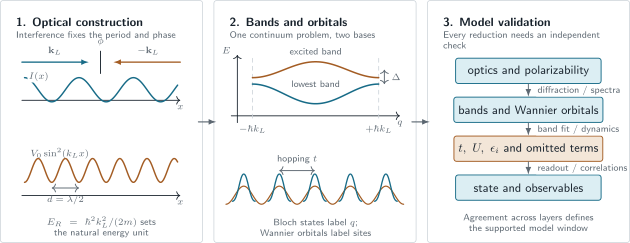
An optical lattice is a hierarchy, not merely a standing-wave picture. Interference fixes the period $d$ and optical potential; the continuum Schrödinger problem fixes bands, gaps, and Wannier orbitals; projection proposes $t$, $U$, and site energies; independent calibration and observables test whether that reduced model is adequate.

Recoil Units and Reciprocal Momentum

For the counterpropagating lattice,

$$d=\frac{\lambda}{2}, \qquad G=\frac{2\pi}{d}=2k_L.$$

The periodic potential contains Fourier components at $\pm G=\pm2k_L$. It therefore couples plane-wave momentum states that differ by

$$\Delta p = \pm2\hbar k_L.$$

The conventional recoil energy nevertheless uses the one-photon momentum $\hbar k_L$:

$$E_R = \frac{\hbar^2k_L^2}{2m}, \qquad \omega_R = \frac{E_R}{\hbar}, \qquad f_R = \frac{E_R}{h}.$$

This convention is useful because the free-particle states that become degenerate at the first Brillouin-zone edge have momenta $\pm\hbar k_L$ and kinetic energy $E_R$.

Useful dimensionless quantities include

$$s=\frac{V_0}{E_R}, \qquad \frac{k_{\mathrm B}T}{E_R}, \qquad \frac{\hbar\omega}{E_R}, \qquad \frac{F d}{E_R}.$$

At fixed wavelength, heavier particles have smaller $E_R$. The same optical depth in hertz can therefore represent a different value of $s$ for another isotope or molecule.

The Single-Particle Band Problem

Dimensionless Schrödinger equation

For one dimension,

$$\left[ - \frac{\hbar^2}{2m} \frac{d^2}{dx^2} + V_0\sin^2(k_Lx) \right]\psi(x) = E\psi(x).$$

Using $u=k_Lx$ and dividing by $E_R$ gives

$$\left[ - \frac{d^2}{du^2} + s\sin^2u \right]\psi(u) = \frac{E}{E_R}\psi(u).$$

This is a Mathieu-type eigenvalue problem. Once energy is measured in $E_R$, its band structure depends only on $s$ for the ideal one-dimensional sinusoidal lattice.

Bloch theorem gives

$$\psi_{nq}(x) = e^{iqx/\hbar}u_{nq}(x), \qquad u_{nq}(x+d)=u_{nq}(x),$$

with

$$-\hbar k_L \le q < \hbar k_L.$$

The band index $n$ records distinct eigenvalues at the same quasimomentum. Quasimomentum is conserved by a perfectly translation-invariant static lattice, but ordinary mechanical momentum is not.

Plane-wave matrix

A direct numerical route expands

$$\psi_q(x) = \sum_{\ell} c_\ell \exp\!\left[ \frac{i}{\hbar} \left(q+2\ell\hbar k_L\right)x \right].$$

Because

$$V_0\sin^2(k_Lx) = \frac{V_0}{2} - \frac{V_0}{4} \left( e^{2ik_Lx} + e^{-2ik_Lx} \right),$$

the dimensionless matrix is tridiagonal:

$$\begin{aligned} \frac{H_{\ell\ell}}{E_R} &= \left( \frac{q}{\hbar k_L}+2\ell \right)^2 + \frac{s}{2}, \\ \frac{H_{\ell,\ell\pm1}}{E_R} &= - \frac{s}{4}. \end{aligned}$$

Convergence is checked by increasing the plane-wave cutoff. This small matrix calculation is often more reliable than applying a deep-lattice asymptotic formula at a moderate value of $s$.

Weak-lattice gap

At $s=0$, the free states with momenta $+\hbar k_L$ and $-\hbar k_L$ are degenerate at the Brillouin-zone edge. The Fourier component $-V_0/4$ couples them. Degenerate perturbation theory gives the matrix

$$\begin{pmatrix} E_R+V_0/2 & -V_0/4\\ -V_0/4 & E_R+V_0/2 \end{pmatrix},$$

so the leading band gap is

$$\Delta_{\mathrm{edge}} \simeq \frac{V_0}{2} \qquad (V_0\ll E_R).$$

The gap is not $V_0$ because $V_0$ is a real-space peak-to-trough depth, whereas the avoided crossing is set by a Fourier matrix element.

Deep-lattice onsite motion

Near a minimum,

$$\sin^2(k_Lx) \simeq k_L^2x^2.$$

Matching $V_0k_L^2x^2$ to $m\omega_{\mathrm{ho}}^2x^2/2$ gives

$$\omega_{\mathrm{ho}} = \frac{2}{\hbar} \sqrt{V_0E_R},$$

or

$$\hbar\omega_{\mathrm{ho}} = 2\sqrt{s}\,E_R.$$

This scale approximates the separation of low onsite vibrational levels, not the exact gap everywhere in the Brillouin zone. Anharmonicity lowers the spacing for higher local levels, and tunneling broadens each onsite level into a band.

The harmonic-oscillator length is

$$a_{\mathrm{ho}} = \sqrt{\frac{\hbar}{m\omega_{\mathrm{ho}}}} = \frac{1}{k_Ls^{1/4}}.$$

It shrinks only as $s^{-1/4}$ even though tunneling falls much more rapidly.

Wannier Orbitals and Tight Binding

For an isolated band, a localized Wannier orbital may be constructed from Bloch states:

$$w_j(x) = \frac{1}{\sqrt{N_s}} \sum_q e^{-iqR_j/\hbar} \psi_{0q}(x), \qquad R_j=jd.$$

The phase choice of $\psi_{0q}$ affects the shape and center of the Wannier function, though not the band energies. In a simple isolated one-dimensional band, phases can be chosen to make well-localized real orbitals. Composite or topological bands require more care.

Projecting the one-particle Hamiltonian into these orbitals gives hopping matrix elements

$$t_{ij} = - \int dx\, w_i^*(x) \left[ - \frac{\hbar^2}{2m} \frac{d^2}{dx^2} + V_{\mathrm{lat}}(x) \right] w_j(x).$$

If only nearest neighbors matter,

$$E_0(q) \simeq \epsilon_0 - 2t \cos\!\left(\frac{qd}{\hbar}\right).$$

The lowest-band width is then

$$W = E_0(\hbar k_L)-E_0(0) \simeq 4t.$$

Near the band minimum,

$$E_0(q) \simeq E_0(0) + \frac{q^2}{2m^*},$$

with

$$m^* = \frac{\hbar^2}{2td^2} \qquad \text{for nearest-neighbor hopping}.$$

A measured width or curvature can therefore determine $t$ only after the assumed hopping range has been tested. If next-nearest-neighbor hopping is appreciable, one number does not determine the full dispersion.

Deep-lattice tunneling estimate

For $s\gg1$, the lowest-band nearest-neighbor hopping has the asymptotic form

$$\frac{t}{E_R} \simeq \frac{4}{\sqrt{\pi}} s^{3/4} e^{-2\sqrt{s}}.$$

Its exponential dependence is physically important: moderate depth changes can alter dynamical time scales by orders of magnitude. The formula is not an exact calibration curve. At experimentally common moderate depths, diagonalizing the actual periodic potential can shift $t$ by tens of percent.

From a Continuum Gas to a Hubbard Candidate

For one internal component of a dilute gas, begin from

$$\begin{aligned} \hat H ={}& \int d^3r\, \hat\Psi^\dagger(\mathbf r) \left[ - \frac{\hbar^2\nabla^2}{2m} + V_{\mathrm{lat}}(\mathbf r) + V_{\mathrm{ext}}(\mathbf r) \right] \hat\Psi(\mathbf r) \\ &+ \frac{g}{2} \int d^3r\, \hat\Psi^\dagger \hat\Psi^\dagger \hat\Psi \hat\Psi. \end{aligned}$$

For a three-dimensional dilute gas with a contact interaction,

$$g = \frac{4\pi\hbar^2a_s}{m}.$$

If the lowest band is isolated and interaction-induced orbital deformation is small, expand

$$\hat\Psi(\mathbf r) \simeq \sum_i w_i(\mathbf r)\hat a_i.$$

The leading parameter dictionary is

$$\begin{aligned} t_{ij} &= - \int d^3r\, w_i^* \left[ - \frac{\hbar^2\nabla^2}{2m} + V_{\mathrm{lat}} \right] w_j, \\ U &= g \int d^3r\, \lvert w_i\rvert^4, \\ \epsilon_i &= \int d^3r\, \lvert w_i\rvert^2 V_{\mathrm{ext}}. \end{aligned}$$

For bosons, the onsite interaction contributes $U\hat n_i(\hat n_i-1)/2$. For a two-component Fermi gas, the leading $s$-wave term is $U\hat n_{i\uparrow}\hat n_{i\downarrow}$. The canonical model pages derive the corresponding Hamiltonians and conventions.

What the optical knobs really control

The controls are correlated:

Experimental control	Leading effect	Coupled consequences
lattice intensity	increases $V_0$	narrows bands, localizes Wannier orbitals, changes $t$ and $U$
wavelength and angle	set $d$ and $E_R$	change band scale, density per site, and optical response
scattering length	changes contact coupling	changes $U$, loss, molecular physics, and multiband mixing
beam phase	translates or shakes the lattice	can heat, drive tunneling, or create inertial forces
polarization	changes state-dependent light shifts	may create spin dependence and Raman scattering
Gaussian envelope	adds smooth confinement	changes filling and local energy offsets
modulation frequency	drives selected transitions	can also produce Floquet bands and heating

Changing the lattice depth does not tune only $t$. It also changes Wannier localization, $U$, the band gap, density-dependent corrections, and sensitivity to noise.

Terms beyond the minimal model

A microscopic projection can generate:

• longer-range and anisotropic hopping;
• density-assisted tunneling;
• pair hopping;
• offsite interactions;
• state-dependent site energies;
• multiple orbitals per site;
• confinement-induced modifications of scattering;
• virtual-band corrections and effective multibody interactions;
• loss terms and time-dependent couplings.

The smallest Hamiltonian is justified by a numerical or experimental error budget, not by the visual regularity of the array.

Loading the Lattice

Single-particle adiabaticity

Suppose the depth is ramped as $V_0(t)$. In an ideal translation-invariant lattice, the ramp preserves quasimomentum and couples bands with the same $q$. A local adiabatic criterion between instantaneous bands is

$$\left| \frac{ \langle m,q;t \vert \partial_t H \vert n,q;t\rangle }{ \left[E_m(q,t)-E_n(q,t)\right]^2 } \right| \hbar \ll1.$$

A ramp slow compared with $\hbar/\Delta_{\mathrm{band}}$ is a useful first intuition, but the matrix element and the minimum gap along the ramp matter. Symmetry can suppress some couplings and imperfections can open others.

Many-body adiabaticity

Avoiding interband excitation does not guarantee that the many-body state remains near its ground state. The relevant gap can instead be:

• a finite-system many-body gap;
• a collective-mode frequency;
• a tunneling scale $t/\hbar$;
• a superexchange scale $4t^2/(\hbar U)$;
• a critical gap that becomes very small near a phase transition;
• an inhomogeneous redistribution time set by transport through the trap.

An experimentally reasonable ramp may therefore be adiabatic with respect to onsite vibrational motion and diabatic with respect to spin or mass transport. The final entropy distribution is part of the result.

Loading sequence

A reproducible loading record should state:

1. species, internal-state mixture, atom number, and initial trap;
2. initial temperature or entropy proxy;
3. lattice wavelengths, geometry, polarization, waists, and detuning;
4. the full time dependence of each lattice axis;
5. simultaneous changes to the smooth confinement and interaction;
6. hold time and any equilibration evidence;
7. depth calibration and its uncertainty;
8. loss, heating, and reversibility checks.

Ramping back to the initial configuration can reveal gross irreversible heating, but return fidelity alone does not prove preparation of the instantaneous many-body ground state.

Release and Momentum Diagnostics

Sudden release

If the lattice is turned off rapidly compared with band dynamics, the localized wave packets are projected onto free momentum states. For a single-band sample, the far-field distribution has the schematic form

$$n(\mathbf k) \propto \lvert\widetilde w(\mathbf k)\rvert^2 \sum_{i,j} e^{i\mathbf k\cdot(\mathbf R_i-\mathbf R_j)} \langle \hat a_i^\dagger\hat a_j \rangle.$$

The Wannier envelope and the one-body density matrix both matter. Interference peaks indicate coherence over multiple sites, but peak visibility alone is not a unique superfluid diagnostic: finite size, temperature, interactions during expansion, imaging resolution, and incoherent backgrounds affect it.

Band mapping

In band mapping, the lattice is ramped down slowly enough to follow an instantaneous Bloch band into a free-particle momentum interval, but fast enough to suppress substantial redistribution from trapping, interactions, or collisions. Symbolically,

$$\tau_{\mathrm{interband}} \ll \tau_{\mathrm{map}} \ll \tau_{\mathrm{redistribution}}.$$

The first inequality prevents transitions between bands; the second attempts to preserve the initial quasimomentum population. There is no universal mapping time. It must be validated for the actual gap, interaction, confinement, and momentum resolution.

Band mapping estimates populations in Brillouin zones. It does not by itself reconstruct phase coherence, interaction energy, or the many-particle density matrix.

Calibrating the Optical Lattice

No single method is reliable in every regime. A mature calibration uses at least one spectroscopic or dynamical method and checks it against the optical power, geometry, and polarizability model.

Optical forward model

The first estimate combines:

• power delivered to each beam at the atoms;
• beam waists and mode quality;
• interference contrast;
• polarization and magnetic-field orientation;
• species- and state-dependent dynamic polarizability;
• window losses and retroreflection efficiency.

This estimate is valuable for diagnosing drifts, but it is often limited by in-vacuum beam parameters. It should not be the only depth calibration.

Kapitza–Dirac diffraction

Apply the lattice for a short pulse $\tau$ to a narrow momentum distribution. In the Raman–Nath limit, kinetic evolution during the pulse is neglected. With

$$V(x) = \frac{V_0}{2} - \frac{V_0}{2}\cos(2k_Lx),$$

the nontrivial part of the pulse operator is

$$U_{\mathrm{KD}} \simeq \exp\!\left[ i\beta\cos(2k_Lx) \right], \qquad \beta = \frac{V_0\tau}{2\hbar}.$$

Using the Jacobi–Anger expansion gives diffraction orders $p=2n\hbar k_L$ with ideal populations

$$P_n = J_n^2(\beta).$$

Fitting several pulse times or several diffraction orders can determine $V_0$. The model fails when kinetic phases, interactions, initial momentum width, pulse-shape errors, or a spatially varying depth are important. The rough requirement $\tau\ll\hbar/E_R$ becomes more restrictive when high diffraction orders are populated.

Modulation spectroscopy

Modulate the depth,

$$V_0(t) = V_0 \left[ 1+\eta\cos(\omega t) \right],$$

or, more transparently,

$$V_0(t) = \bar V_0 + \delta V\cos(\omega t).$$

Excitation resonances constrain band gaps or many-body energy scales. Selection rules depend on whether depth, position, or another parameter is modulated. In a symmetric lattice, pure amplitude modulation has different parity selection rules from phase modulation.

The observed maximum need not equal a bare band gap. Interactions, inhomogeneous broadening, finite pulse duration, nonlinear response, and population-dependent shifts can move or broaden it. Calibration should fit a forward model rather than assign a depth from one peak by eye.

Onsite vibrational spectroscopy

In a deep lattice, transitions between local vibrational levels probe $\omega_{\mathrm{ho}}$ and anharmonic corrections. The harmonic estimate

$$\hbar\omega_{\mathrm{ho}} \simeq 2\sqrt{V_0E_R}$$

provides an initial inversion for $V_0$, while a full band calculation improves the result. Parity and probe geometry determine which transitions are visible.

Tunneling dynamics

Prepare an imbalance, a localized wave packet, or a tilted lattice and observe coherent transport. The oscillation or expansion dynamics can constrain $t$ and longer-range hopping directly. This is often closer to the parameter needed in a Hubbard model than a nominal optical depth is.

Interactions and dephasing must be included. A decay of oscillations does not uniquely measure tunneling; it can arise from trap inhomogeneity, collisions, technical noise, or averaging over different local depths.

Bloch oscillations

Under a uniform force $F$,

$$\dot q = F.$$

Advancing across a Brillouin zone of width $2\pi\hbar/d$ gives the Bloch period

$$T_B = \frac{h}{Fd}.$$

Bloch oscillations accurately connect force, spacing, and quasimomentum dynamics. Their amplitude and waveform can constrain the band dispersion, but the period alone does not determine $V_0$.

Cross-calibration ledger

Method	Primary quantity	Leading model risk
optical power and polarizability	nominal $V_0$	unknown in-vacuum intensity or polarization
Kapitza–Dirac diffraction	pulse area $V_0\tau/\hbar$	breakdown of Raman–Nath dynamics
band or vibrational spectroscopy	energy differences	interactions and inhomogeneous broadening
tunneling dynamics	$t$ and possibly longer-range hopping	dephasing and trap averaging
band mapping	band populations	incompatible ramp time scales
Bloch oscillations	$Fd$ and dispersion response	Landau–Zener loss and confinement

Agreement among methods tests more than statistical precision. A systematic disagreement can reveal imperfect contrast, multiband occupation, an incorrect polarizability, or a nonseparable potential.

Worked Scale Audit: Rubidium at 1064 nm

Consider $^{87}\mathrm{Rb}$ in a one-dimensional $\lambda=1064\,\mathrm{nm}$ lattice with

$$s = \frac{V_0}{E_R} = 8.$$

Using $m=86.9091805\,u$ gives

$$\begin{aligned} d &= 532\,\mathrm{nm}, \\ \frac{E_R}{h} &\simeq 2.028\,\mathrm{kHz}, \\ \frac{E_R}{k_{\mathrm B}} &\simeq 97.3\,\mathrm{nK}. \end{aligned}$$

The harmonic onsite estimate is

$$\frac{\omega_{\mathrm{ho}}}{2\pi} = 2\sqrt{s} \frac{E_R}{h} \simeq 11.47\,\mathrm{kHz}.$$

A converged plane-wave diagonalization of the ideal sinusoidal potential gives, for the lowest band,

$$\frac{W}{E_R} \simeq 0.12328.$$

If nearest-neighbor hopping dominates,

$$\frac{t}{E_R} \simeq \frac{W}{4E_R} = 0.03082,$$

so

$$\frac{t}{h} \simeq 62.5\,\mathrm{Hz}, \qquad \frac{h}{t} \simeq 16.0\,\mathrm{ms}.$$

By comparison, the deep-lattice asymptotic formula gives

$$\frac{t_{\mathrm{asym}}}{E_R} \simeq 0.03750,$$

about $22\%$ above the plane-wave result. The example is deliberately at a moderate depth: it shows why an asymptotic expression is a scale check, not a precision calibration.

For the same ideal calculation, the minimum gap from the lowest to the first excited band occurs at the zone edge and is approximately

$$\frac{\Delta_{01}^{\min}}{E_R} \simeq 3.770,$$

or $\Delta_{01}^{\min}/h\simeq7.64\,\mathrm{kHz}$. This is comfortably larger than $t/h$, but a drive, interaction energy, or ramp rate must be compared with the gap independently.

Heating and Coherence Limits

Photon scattering

The same optical susceptibility that creates the conservative potential has an absorptive part. Off-resonant scattering can:

• add recoil energy;
• change hyperfine or Zeeman states through Raman processes;
• dephase superpositions;
• eject particles from shallow bands or traps;
• create density-dependent loss after state changes.

The scattering rate is species-, wavelength-, polarization-, and state-dependent. It cannot be inferred from $s$ alone. The canonical Optical Dipole Traps page gives the polarizability and fixed-depth detuning trade-off.

Intensity noise

Depth noise changes:

$$V_0(t), \qquad \omega_{\mathrm{ho}}(t), \qquad t(t), \qquad U(t).$$

Noise near twice an onsite trap frequency can drive parametric heating. Low-frequency drift changes the Hamiltonian between shots. Because $t$ depends exponentially on $\sqrt{s}$ in a deep lattice, a small depth fluctuation can become a much larger fractional tunneling fluctuation.

Phase and frequency noise

Relative phase noise translates the lattice. It can excite dipole motion, drive interband transitions, or appear as an inertial force in the lattice frame. Relative frequency noise integrates into phase noise and can cause uncontrolled lattice velocity.

The relevant specification is the phase-noise spectrum at the atoms, including optical path motion after any common reference point. A narrow laser linewidth does not guarantee a stable retroreflected standing wave.

Beam geometry noise

Pointing, waist, focus, and angle drift alter both the periodic depth and the smooth envelope. In multidimensional lattices they can change anisotropy and relative sublattice registration. Diagnostics should therefore monitor more than total power.

Interaction-induced heating and loss

Strong interactions can mix higher orbitals, generate doublons with large loss rates, or make an otherwise slow ramp diabatic. Near a Feshbach resonance, the scattering length alone may not describe onsite few-body physics. Molecules, effective range, confinement-induced resonances, and three-body channels may enter.

Floquet heating

Periodic shaking or modulation can engineer complex hopping and effective gauge fields. The effective Floquet Hamiltonian is useful only within a frequency and time window. Resonant coupling to higher bands, micromotion, interaction-assisted absorption, and eventual heating must be reported alongside the engineered parameter.

Validity of a Single-Band Lattice Model

Before using a one-band Hamiltonian, compare the following scales:

$$k_{\mathrm B}T,\quad t,\quad U,\quad \hbar\omega_{\mathrm{drive}},\quad Fd,\quad \hbar\Gamma_{\mathrm{heat}}$$

with the minimum relevant band gap $\Delta_{\mathrm{band}}$. A conservative starting requirement is

$$k_{\mathrm B}T,\, \lvert t\rvert,\, \lvert U\rvert,\, \hbar\omega_{\mathrm{drive}},\, \lvert Fd\rvert \ll \Delta_{\mathrm{band}},$$

but this list is not sufficient:

1. Band isolation: occupation and virtual mixing of higher bands are below the target error.
2. Orbital stability: interactions do not substantially deform the retained Wannier orbital.
3. Hopping truncation: omitted longer-range matrix elements are small for the measured dynamics.
4. Interaction truncation: offsite, density-assisted, and multibody terms are bounded.
5. Spatial model: the Gaussian envelope, disorder, and compensating potentials are included or shown negligible.
6. Internal-state model: scalar, vector, tensor, and Raman light shifts match the assumed spin Hamiltonian.
7. Open-system window: loss and heating are slow compared with the observation time.
8. Preparation: the state, not only the Hamiltonian, is characterized.
9. Readout: the detector response is connected to the quoted observable.
10. Parameter covariance: uncertainties in $V_0$, $a_s$, geometry, and filling are propagated jointly.

The ratio $\Delta_{\mathrm{band}}/U$ is not the only multiband diagnostic. Even off-resonant virtual excitations can renormalize low-energy parameters before producing visible higher-band population.

Quantum Simulation

Analog simulation

An analog quantum simulator prepares a controllable Hamiltonian whose low-energy dynamics approximate a target model. Optical lattices are especially useful because geometry, hopping, interaction, dimension, filling, and observation time can often be varied independently enough to test model predictions.

They are not perfectly independent knobs. The mapping from laboratory controls $\boldsymbol\lambda$ to model parameters $\boldsymbol\theta$ should be treated as a calibrated function,

$$\boldsymbol\theta = \mathcal M(\boldsymbol\lambda),$$

with an uncertainty matrix and a validity domain.

Bosonic Hubbard physics

Bosons in a sufficiently isolated lowest band can realize the Bose–Hubbard competition between tunneling and onsite repulsion. The observation of a superfluid-to-Mott crossover in a trapped gas established optical lattices as a central quantum-simulation platform.

That historical result should not be reduced to disappearing interference peaks. A Mott claim is strengthened by number squeezing, suppressed compressibility, a particle-hole gap, and consistency with trap inhomogeneity. The Bose–Hubbard Model develops those diagnostics.

Fermionic Hubbard physics

A two-component Fermi gas can realize hopping, onsite interactions, doublons, local moments, and spin correlations of the fermionic Hubbard model. The low-energy antiferromagnetic exchange scale in the repulsive strong-coupling regime is

$$J_{\mathrm{ex}} \simeq \frac{4t^2}{U}.$$

Preparing a gas with $T<T_{\mathrm F}$ before loading is not enough: magnetic correlations require entropy and temperature low on the exchange scale. Degenerate Fermi Gases Overview explains the continuum preparation, while the Hubbard Model owns the lattice many-body physics.

Engineered bands and gauge fields

Additional controls can produce:

• superlattices and double wells;
• spin-dependent lattices;
• Raman-assisted or laser-assisted hopping;
• Peierls phases and synthetic magnetic flux;
• shaken-lattice Floquet bands;
• synthetic dimensions;
• quasiperiodic and disordered potentials;
• topological band structures.

Each extension enlarges the calibration problem. For example, a measured band topology does not establish that interactions are negligible, and a target Peierls phase must be distinguished from uncontrolled micromotion and spatial phase gradients.

Digital and programmable use

Deep lattices can isolate particles for local control, collisional gates, state preparation, or microscope readout. A conventional optical lattice is periodic rather than site-programmable, but superlattices, spatial light modulators, local addressing, and digital micromirror devices can add structure. Optical tweezers provide a complementary route when arbitrary site placement and rearrangement matter more than translational symmetry.

Observables and Evidence

Different measurements establish different statements:

Measurement	Directly constrains	Does not alone establish
diffraction or band mapping	momentum or band populations	equilibrium or superfluidity
modulation spectrum	response at an energy scale	unique microscopic origin without a model
center-of-mass transport	mobility and dispersion response	local correlations
doublon fraction	onsite pair occupation	a complete phase diagnosis
compressibility	density response	magnetic order
noise correlations	momentum-space two-point structure	arbitrary real-space correlators
site-resolved fluorescence	detected site occupations	pre-detection occupation without loss correction
spin correlations	magnetic structure over measured ranges	thermodynamic long-range order automatically

Quantum gas microscopes add spatial resolution but not infallibility. Light-assisted collisions can produce parity projection; hopping or loss during imaging can alter occupations; internal-state readout has a confusion matrix. The forward measurement channel belongs in the scientific model.

Validation ladder

A strong lattice-simulation claim includes:

1. apparatus validation: wavelength, geometry, polarization, phase stability, and intensity at the atoms;
2. single-particle validation: bands, gaps, tunneling, and higher-band population;
3. interaction validation: scattering parameters, doublon or spectroscopy checks, and loss;
4. state validation: filling, temperature or entropy, spatial inhomogeneity, and preparation history;
5. observable validation: detector response and uncertainty;
6. model discrimination: at least one measurement sensitive to an important omitted term;
7. cross-regime checks: known limits such as noninteracting, atomic, or weak-drive behavior.

Agreement with a difficult many-body prediction is persuasive only when the easier calibration layers are also under control.

Common Mistakes

Calling the spacing the optical wavelength

Counterpropagating equal-frequency beams produce $d=\lambda/2$, not $d=\lambda$. A noncounterpropagating geometry gives $d=\lambda/[2\sin(\theta/2)]$.

Confusing recoil and reciprocal-lattice momentum

The potential transfers momentum in units of $2\hbar k_L$, while $E_R$ is defined from $\hbar k_L$. Both conventions are correct and refer to different quantities.

Treating depth as a frequency without Planck’s constant

Statements such as “$V_0=10\,\mathrm{kHz}$” should mean either $V_0/h=10\,\mathrm{kHz}$ or $V_0/\hbar=2\pi\times10\,\mathrm{kHz}$. The distinction is a factor of $2\pi$.

Equating deep wells with a one-band model

Deepening the lattice suppresses hopping and increases onsite level spacing, but strong interactions, rapid drives, or lossy onsite states can still invalidate a single-band reduction.

Using the harmonic frequency as the band gap

$2\sqrt{s}E_R/\hbar$ is a local deep-well estimate. Exact gaps depend on quasimomentum and anharmonicity.

Inferring tunneling from an asymptotic formula at moderate depth

The exponential formula is valuable for scaling. Precision work should diagonalize the measured potential or calibrate dynamics.

Calling every periodic gas a Hubbard simulator

A Hubbard claim requires a controlled Wannier projection, quantified omitted terms, calibrated $t$ and $U$, known filling and temperature, and observables that test the model.

Calling a loading ramp adiabatic

Adiabatic relative to the band gap may still be diabatic relative to tunneling, spin exchange, a critical gap, or redistribution through an inhomogeneous trap.

Reading time-of-flight peaks as a phase label

Interference peaks probe one-body coherence with a Wannier envelope and a measurement transfer function. They do not alone establish thermodynamic superfluidity or exclude an inhomogeneous mixture of phases.

Ignoring the smooth envelope

The lattice is periodic on short scales and usually inhomogeneous on long scales. Filling, local chemical potential, tunneling, and even depth can vary across the cloud.

Experimental Audit Workflow

For a proposed optical-lattice experiment:

1. Declare geometry. Record all wave vectors, wavelengths, frequency offsets, polarizations, phases, waists, and retroreflection paths.
2. Calculate the optical potential. Use the correct multilevel polarizability and interference contrast.
3. Choose units. Report $d$, $E_R/h$, $V_0/E_R$, and the quasimomentum convention.
4. Solve the single-particle problem. Compute bands, minimum gaps, Wannier orbitals, and more than one hopping range.
5. Project interactions. Calculate candidate onsite and offsite terms with confinement corrections where necessary.
6. Calibrate independently. Use diffraction, spectroscopy, tunneling, or another validated dynamical method.
7. Audit loading. Compare the ramp with band, tunneling, interaction, exchange, transport, and critical scales.
8. Measure heating. Determine loss and energy growth versus hold time, depth, and technical noise.
9. Characterize the state. Report filling, inhomogeneity, band populations, temperature or entropy proxy, and preparation history.
10. Validate the detector. Include parity projection, loss, misclassification, and resolution.
11. Test an omitted term. Vary a control that changes higher-band, longer-range, or envelope corrections.
12. Report a model window. State the observables, times, energies, and parameter range for which the reduced Hamiltonian is supported.

Canonical Connections

• Analog Quantum Simulation supplies the platform-independent encoding, effective-Hamiltonian, observable-error, resource, and validation framework used by this optical lattice implementation.
• Artificial Lattices and Designer Matter compares optical-lattice analogs with quantum-dot, photonic, polaritonic, circuit, and assembled-electron platforms through a shared validation ledger.
• Optical Clocks develops magic-wavelength clock operation, residual lattice shifts, neutral-atom interactions, optical-ratio comparison, and relativistic applications.
• Optical Dipole Traps develops the general potential, scattering, and technical-heating framework.
• AC Stark Shift derives state-dependent optical potentials from atomic dressing.
• Bloch Theorem gives the translation-symmetry statement behind quasimomentum and bands.
• Tight-Binding Model owns hopping Hamiltonians, dispersions, and boundary conventions.
• Bose–Hubbard Model owns bosonic onsite interactions and the superfluid–Mott structure.
• Hubbard Model owns the two-component fermionic model and its strong-coupling limits.
• Bose–Einstein Condensates Overview supplies condensate preparation and coherence diagnostics.
• Degenerate Fermi Gases Overview supplies fermionic preparation, Feshbach tuning, and entropy-scale context.
• AMO Model Index contrasts single-band Hubbard reductions with continuum Gross–Pitaevskii and center-of-mass control models.

References

1. R. Grimm, M. Weidemüller, and Y. B. Ovchinnikov, “Optical Dipole Traps for Neutral Atoms,” Advances in Atomic, Molecular, and Optical Physics 42, 95–170 (2000), doi:10.1016/S1049-250X(08)60186-X.
2. O. Morsch and M. Oberthaler, “Dynamics of Bose–Einstein Condensates in Optical Lattices,” Reviews of Modern Physics 78, 179–215 (2006), doi:10.1103/RevModPhys.78.179.
3. I. Bloch, J. Dalibard, and W. Zwerger, “Many-Body Physics with Ultracold Gases,” Reviews of Modern Physics 80, 885–964 (2008), doi:10.1103/RevModPhys.80.885.
4. M. Lewenstein, A. Sanpera, V. Ahufinger, B. Damski, A. Sen De, and U. Sen, “Ultracold Atomic Gases in Optical Lattices: Mimicking Condensed Matter Physics and Beyond,” Advances in Physics 56, 243–379 (2007), doi:10.1080/00018730701223200.
5. D. Jaksch, C. Bruder, J. I. Cirac, C. W. Gardiner, and P. Zoller, “Cold Bosonic Atoms in Optical Lattices,” Physical Review Letters 81, 3108–3111 (1998), doi:10.1103/PhysRevLett.81.3108.
6. W. Zwerger, “Mott–Hubbard Transition of Cold Atoms in Optical Lattices,” Journal of Optics B: Quantum and Semiclassical Optics 5, S9–S16 (2003), doi:10.1088/1464-4266/5/2/352.
7. Y. B. Ovchinnikov, J. H. Müller, M. R. Doery, E. J. D. Vredenbregt, K. Helmerson, S. L. Rolston, and W. D. Phillips, “Diffraction of a Released Bose–Einstein Condensate by a Pulsed Standing Light Wave,” Physical Review Letters 83, 284–287 (1999), doi:10.1103/PhysRevLett.83.284.
8. M. Greiner, O. Mandel, T. Esslinger, T. W. Hänsch, and I. Bloch, “Quantum Phase Transition from a Superfluid to a Mott Insulator in a Gas of Ultracold Atoms,” Nature 415, 39–44 (2002), doi:10.1038/415039a.
9. T. Stöferle, H. Moritz, C. Schori, M. Köhl, and T. Esslinger, “Transition from a Strongly Interacting 1D Superfluid to a Mott Insulator,” Physical Review Letters 92, 130403 (2004), doi:10.1103/PhysRevLett.92.130403.
10. M. Köhl, H. Moritz, T. Stöferle, K. Günter, and T. Esslinger, “Fermionic Atoms in a Three Dimensional Optical Lattice: Observing Fermi Surfaces, Dynamics, and Interactions,” Physical Review Letters 94, 080403 (2005), doi:10.1103/PhysRevLett.94.080403.
11. R. Jördens, N. Strohmaier, K. Günter, H. Moritz, and T. Esslinger, “A Mott Insulator of Fermionic Atoms in an Optical Lattice,” Nature 455, 204–207 (2008), doi:10.1038/nature07244.
12. U. Schneider, L. Hackermüller, S. Will, T. Best, I. Bloch, T. A. Costi, R. W. Helmes, D. Rasch, and A. Rosch, “Metallic and Insulating Phases of Repulsively Interacting Fermions in a 3D Optical Lattice,” Science 322, 1520–1525 (2008), doi:10.1126/science.1165449.
13. T. Esslinger, “Fermi–Hubbard Physics with Atoms in an Optical Lattice,” Annual Review of Condensed Matter Physics 1, 129–152 (2010), doi:10.1146/annurev-conmatphys-070909-104059.
14. W. S. Bakr, J. I. Gillen, A. Peng, S. Fölling, and M. Greiner, “A Quantum Gas Microscope for Detecting Single Atoms in a Hubbard-Regime Optical Lattice,” Nature 462, 74–77 (2009), doi:10.1038/nature08482.
15. J. F. Sherson, C. Weitenberg, M. Endres, M. Cheneau, I. Bloch, and S. Kuhr, “Single-Atom-Resolved Fluorescence Imaging of an Atomic Mott Insulator,” Nature 467, 68–72 (2010), doi:10.1038/nature09378.
16. L. W. Cheuk, M. A. Nichols, M. Okan, T. Gersdorf, V. V. Ramasesh, W. S. Bakr, T. Lompe, and M. W. Zwierlein, “Quantum-Gas Microscope for Fermionic Atoms,” Physical Review Letters 114, 193001 (2015), doi:10.1103/PhysRevLett.114.193001.
17. A. Mazurenko, C. S. Chiu, G. Ji, M. F. Parsons, M. Kanász-Nagy, R. Schmidt, F. Grusdt, E. Demler, D. Greif, and M. Greiner, “A Cold-Atom Fermi–Hubbard Antiferromagnet,” Nature 545, 462–466 (2017), doi:10.1038/nature22362.
18. R. P. Feynman, “Simulating Physics with Computers,” International Journal of Theoretical Physics 21, 467–488 (1982), doi:10.1007/BF02650179.

Exercises

1. Fringe spacing and phase translation

Two equal-frequency beams of wavelength $\lambda=780\,\mathrm{nm}$ cross at $\theta=60^\circ$.

1. Find the fringe spacing.
2. If the relative optical phase increases by $\pi/3$, how far does the pattern translate along the interference wave vector?
3. Compare with counterpropagating beams at the same wavelength.

Solution

The interference-wave-vector magnitude is

$$\lvert\Delta\mathbf k\rvert = 2k_L\sin\!\left(\frac{\theta}{2}\right).$$

Therefore

$$\begin{aligned} d &= \frac{\lambda}{2\sin(\theta/2)} \\ &= \frac{780\,\mathrm{nm}} {2\sin30^\circ} \\ &= 780\,\mathrm{nm}. \end{aligned}$$

A phase change translates the pattern by

$$\delta x = \frac{\delta\phi}{\lvert\Delta\mathbf k\rvert} = \frac{\delta\phi}{2\pi}d.$$

For $\delta\phi=\pi/3$,

$$\delta x = \frac{d}{6} = 130\,\mathrm{nm}.$$

For counterpropagating beams, $\theta=\pi$, so

$$d_{\mathrm{counter}} = \frac{\lambda}{2} = 390\,\mathrm{nm}.$$

The same phase change then translates the lattice by $d_{\mathrm{counter}}/6=65\,\mathrm{nm}$.

2. Weak-lattice band gap

For

$$V(x) = V_0\sin^2(k_Lx),$$

use the free states $\lvert+\hbar k_L\rangle$ and $\lvert-\hbar k_L\rangle$ to derive the leading gap at the first Brillouin-zone edge. Explain why the answer is not $V_0$.

Solution

The Fourier expansion is

$$V(x) = \frac{V_0}{2} - \frac{V_0}{4} e^{2ik_Lx} - \frac{V_0}{4} e^{-2ik_Lx}.$$

The constant shifts both free states equally. The components at $\pm2k_L$ couple states whose momenta differ by $2\hbar k_L$. In the degenerate subspace,

$$H_{\mathrm{edge}} = \begin{pmatrix} E_R+V_0/2 & -V_0/4\\ -V_0/4 & E_R+V_0/2 \end{pmatrix}.$$

Its eigenvalues are

$$E_\pm = E_R+\frac{V_0}{2} \pm \frac{V_0}{4}.$$

Hence

$$\Delta_{\mathrm{edge}} = E_+-E_- = \frac{V_0}{2}.$$

The real-space peak-to-trough depth $V_0$ is not the coupling matrix element. The avoided crossing is set by the Fourier amplitude $\lvert V_G\rvert=V_0/4$, and the two-level splitting is $2\lvert V_G\rvert=V_0/2$.

3. Onsite oscillator scale

Expand a lattice well near a minimum and show that

$$\hbar\omega_{\mathrm{ho}} = 2\sqrt{s}\,E_R.$$

Find $a_{\mathrm{ho}}/d$ at $s=16$.

Solution

Near $x=0$,

$$V_0\sin^2(k_Lx) \simeq V_0k_L^2x^2.$$

Equating this with $m\omega_{\mathrm{ho}}^2x^2/2$ gives

$$\omega_{\mathrm{ho}}^2 = \frac{2V_0k_L^2}{m}.$$

Since

$$E_R = \frac{\hbar^2k_L^2}{2m},$$

one obtains

$$\omega_{\mathrm{ho}} = \frac{2\sqrt{V_0E_R}}{\hbar} = \frac{2\sqrt{s}\,E_R}{\hbar}.$$

The oscillator length is

$$a_{\mathrm{ho}} = \frac{1}{k_Ls^{1/4}}.$$

Because $d=\pi/k_L$,

$$\frac{a_{\mathrm{ho}}}{d} = \frac{1}{\pi s^{1/4}}.$$

At $s=16$, $s^{1/4}=2$, so

$$\frac{a_{\mathrm{ho}}}{d} = \frac{1}{2\pi} \simeq 0.159.$$

This is a harmonic estimate for the local orbital width, not an exact Wannier-function result.

4. Kapitza–Dirac populations

A short lattice pulse has

$$\beta = \frac{V_0\tau}{2\hbar} = 1.$$

Using $J_0(1)\simeq0.7652$, $J_1(1)\simeq0.4401$, and $J_2(1)\simeq0.1149$, estimate the populations in the orders $n=0,\pm1,\pm2$. Check the partial normalization and state where the remaining probability resides.

Solution

The ideal Raman–Nath populations are

$$P_n = J_n^2(\beta).$$

Therefore

$$\begin{aligned} P_0 &\simeq (0.7652)^2 = 0.5855, \\ P_{+1}=P_{-1} &\simeq (0.4401)^2 = 0.1937, \\ P_{+2}=P_{-2} &\simeq (0.1149)^2 = 0.0132. \end{aligned}$$

The included orders sum to

$$P_0+2P_1+2P_2 \simeq 0.9993.$$

The remaining probability, about $7\times10^{-4}$ with the rounded Bessel values, lies in $\lvert n\rvert\ge3$ and in rounding error. The momenta are $p_n=2n\hbar k_L$.

If the pulse is not short enough, the observed populations are not given by these Bessel squares because kinetic phases accumulate during the pulse.

5. Band width, tunneling, and effective mass

The lowest band of a one-dimensional lattice has measured width $W/h=240\,\mathrm{Hz}$. Assume a nearest-neighbor cosine band and lattice spacing $d=500\,\mathrm{nm}$.

1. Find $t/h$.
2. Find $m^*/m_e$, where $m_e$ is the electron mass.
3. Name one observation that could falsify the nearest-neighbor assumption.

Solution

For

$$E(q) = \epsilon_0 - 2t\cos(qd/\hbar),$$

the width is $W=4t$. Hence

$$\frac{t}{h} = \frac{W}{4h} = 60\,\mathrm{Hz}.$$

The effective mass is

$$m^* = \frac{\hbar^2}{2td^2}.$$

Using $t=h(60\,\mathrm{Hz})$ and $d=5.00\times10^{-7}\,\mathrm m$ gives

$$m^* \simeq 5.60\times10^{-25}\,\mathrm{kg}.$$

Therefore

$$\frac{m^*}{m_e} \simeq \frac{5.60\times10^{-25}} {9.109\times10^{-31}} \simeq 6.15\times10^5.$$

This comparison does not imply that the atom has become an electron-like particle; it compares the curvature of one band with a free-particle mass.

Measuring the dispersion at several quasimomenta can falsify the pure cosine form. A significant $\cos(2qd/\hbar)$ harmonic would reveal next-nearest-neighbor hopping. Real-space dynamics sensitive to multiple hopping distances provide another test.

6. Audit the 1064 nm scale example

For $^{87}\mathrm{Rb}$ at $\lambda=1064\,\mathrm{nm}$ and $s=8$:

1. use $E_R/h=2.028\,\mathrm{kHz}$ to find $V_0/h$;
2. use the exact-band value $t/E_R=0.03082$ to find $t/h$ and $h/t$;
3. compare with the asymptotic value $t/E_R=0.03750$;
4. explain which value should be used in a precision analysis.

Solution

The depth is

$$\frac{V_0}{h} = s\frac{E_R}{h} = 8(2.028\,\mathrm{kHz}) = 16.22\,\mathrm{kHz}.$$

For the exact sinusoidal-band calculation,

$$\frac{t}{h} = 0.03082(2.028\,\mathrm{kHz}) \simeq 62.5\,\mathrm{Hz}.$$

Thus

$$\frac{h}{t} = \frac{1}{62.5\,\mathrm{Hz}} \simeq 16.0\,\mathrm{ms}.$$

The asymptotic estimate gives

$$\frac{t_{\mathrm{asym}}}{h} = 0.03750(2.028\,\mathrm{kHz}) \simeq 76.1\,\mathrm{Hz}.$$

Its relative excess is

$$\frac{76.1-62.5}{62.5} \simeq 0.218,$$

or about $22\%$.

For the ideal sine-squared potential, use a converged band calculation. For a real apparatus, use the measured potential and an independently calibrated tunneling observable when possible. The asymptotic formula is appropriate for intuition and deep-lattice scaling, not as the sole precision input at $s=8$.

7. Single-band decision

An experiment reports

$$\begin{aligned} \frac{\Delta_{\mathrm{band}}}{h} &= 8.0\,\mathrm{kHz}, & \frac{t}{h} &= 100\,\mathrm{Hz}, \\ \frac{U}{h} &= 2.0\,\mathrm{kHz}, & \frac{k_{\mathrm B}T}{h} &= 600\,\mathrm{Hz}. \end{aligned}$$

It applies amplitude modulation with $\omega_{\mathrm{drive}}/(2\pi)=6.5\,\mathrm{kHz}$ and observes for $200\,\mathrm{ms}$ while the measured heating time is $1.5\,\mathrm{s}$. Which facts support a single-band equilibrium model, and which require further investigation?

Solution

The static low-energy scales satisfy

$$t,\ k_{\mathrm B}T,\ U < \Delta_{\mathrm{band}},$$

with ratios

$$\frac{t}{\Delta_{\mathrm{band}}} = 0.0125, \qquad \frac{k_{\mathrm B}T}{\Delta_{\mathrm{band}}} = 0.075, \qquad \frac{U}{\Delta_{\mathrm{band}}} = 0.25.$$

Small $t/\Delta_{\mathrm{band}}$ supports a one-band kinetic description. The temperature is also well below the gap. The interaction ratio is not tiny; interaction-induced orbital deformation and virtual-band corrections should be calculated rather than dismissed.

The modulation frequency has

$$\frac{\hbar\omega_{\mathrm{drive}}} {\Delta_{\mathrm{band}}} = \frac{6.5}{8.0} = 0.8125.$$

It approaches the band gap, so the driven experiment may excite higher bands even if the undriven model is one band. The drive matrix element, band dispersion, pulse spectrum, and observed higher-band population need measurement.

The observation-time fraction of the heating time is

$$\frac{0.2}{1.5} \simeq 0.13.$$

That is not automatically negligible. One should measure the actual energy or entropy increase over $200\,\mathrm{ms}$ and compare it with the required accuracy.

Finally, none of these ratios establishes equilibrium. Loading adiabaticity, redistribution through the trap, filling, and detector calibration remain separate questions.

8. Design a model-validation campaign

A group claims to realize the half-filled repulsive Fermi–Hubbard model and observes short-range antiferromagnetic correlations. Propose a compact validation campaign that distinguishes:

1. a band-calibration error;
2. an error in $U/t$;
3. heating or nonadiabatic loading;
4. trap inhomogeneity;
5. next-nearest-neighbor hopping;
6. a spin-readout error.

Solution

One defensible campaign is:

1. Band calibration: measure lattice depth by band or vibrational spectroscopy and compare it with Kapitza–Dirac diffraction in a weakly interacting sample. Directly measure tunneling dynamics at one or more depths.
2. Interaction calibration: use doublon spectroscopy or two-particle onsite spectroscopy, propagate the scattering-length uncertainty, and compare the inferred $U$ with a Wannier calculation.
3. Heating and loading: vary ramp time and hold time independently. Measure entropy-sensitive observables, higher-band population, loss, and correlation recovery after a reverse ramp.
4. Inhomogeneity: use site-resolved density to reconstruct the local filling and compare correlations in narrow density shells rather than only in a cloud average. Vary compensating confinement.
5. Longer-range hopping: measure the single-particle dispersion or wave-packet dynamics over enough quasimomenta to fit both $t$ and $t'$. Test whether the spin-correlation data change under a depth variation that alters $t'/t$.
6. Spin readout: calibrate the spin-dependent detection confusion matrix with prepared reference states, including loss and hopping during imaging, then unfold or forward-model that channel.

The strongest comparison is simultaneous: use the independently measured parameter covariance and detector channel to predict several observables, including at least one that is sensitive to each suspected correction. Agreement with antiferromagnetic correlations alone cannot distinguish all six failures.

Frontier Context

Ultracold Atom Quantum Simulation tracks current Hubbard-model, gauge-theory, synthetic-dimension, topological, and nonequilibrium results, with explicit attention to thermometry, finite-size evidence, and analog-simulator validation.