Bose–Hubbard Model

The Bose–Hubbard model describes bosons that tunnel between lattice sites and interact when they occupy the same site. In its homogeneous, single-band, nearest-neighbor form, the grand Hamiltonian is

$$\begin{aligned} K ={}& -t \sum_{\langle i,j\rangle} \left( b_i^\dagger b_j + b_j^\dagger b_i \right) \\ &+ \frac{U}{2} \sum_i n_i(n_i-1) - \mu \sum_i n_i, \end{aligned}$$

with $n_i=b_i^\dagger b_i$. The hopping amplitude $t$ rewards delocalization and phase coherence. Repulsive $U>0$ penalizes onsite pairs and suppresses number fluctuations. The chemical potential $\mu$ chooses the equilibrium density when particle exchange is allowed.

This competition produces one of the central phase diagrams of quantum many-body physics. At integer filling, sufficiently strong repulsion supports an incompressible Mott phase even though the Hamiltonian contains no static disorder and no explicit density-wave potential. Increasing $t/U$ restores a compressible superfluid. The short Hamiltonian therefore exposes, in unusually clean form, how interaction and quantum motion can reorganize a many-particle ground state.

Canonical Scope

This page is the canonical home for the single-component Bose–Hubbard model: its Hilbert space, Hamiltonian conventions, symmetries, controlled limits, atomic particle and hole gaps, optical-lattice reduction, observables, and single-site mean-field phase boundary. Lattice Models Overview supplies the shared language of sites, bonds, locality, and effective-model validity.

The Bose–Hubbard Dimer dossier owns the complete two-mode fixed-number problem, including its spin map, exact $N=2$ spectrum, observables, dynamics, and MB-B005 realization. Bose–Hubbard Chain owns the one-dimensional boundary conventions, exact free and hard-core limits, Luttinger-liquid diagnostics, commensurate BKT regime, and finite-chain benchmark. The operator actions and occupation-basis audit rules live in Bosonic Operators in Many-Body Models and Occupation-Number Representation. Quantum Phase Transitions owns the general zero-temperature transition and the detailed distinction between density-driven lobe sides and commensurate lobe tips. Universality owns why those boundary points can belong to different classes. Optical Lattices owns the detailed construction, loading, calibration, and imaging of the experiment; here the optical lattice is used to derive and interpret the effective Hamiltonian.

The Bose–Hubbard Model card remains a compact convention and navigation entry. It points here for the full treatment.

Degrees of Freedom

Choose a lattice or graph with $L$ sites. Each site is a bosonic mode with operators satisfying

$$\begin{aligned} [b_i,b_j^\dagger] &= \delta_{ij}I, \\ [b_i,b_j] &= [b_i^\dagger,b_j^\dagger] =0. \end{aligned}$$

The local number states obey

$$\begin{aligned} n_i\lvert m_i\rangle &= m_i\lvert m_i\rangle, \\ b_i\lvert m_i\rangle &= \sqrt{m_i}\, \lvert m_i-1\rangle, \\ b_i^\dagger\lvert m_i\rangle &= \sqrt{m_i+1}\, \lvert m_i+1\rangle. \end{aligned}$$

Here $n_i$ is the number operator and $m_i$ is its integer eigenvalue. In occupation vectors below, the conventional labels $n_1,\ldots,n_L$ denote eigenvalues. A many-site occupation vector is

$$\lvert n_1,n_2,\ldots,n_L\rangle, \qquad n_i\in\{0,1,2,\ldots\}.$$

Unlike a spin-$1/2$ or fermionic site, a soft-core bosonic site has no finite maximum occupation. The exact local Hilbert space is infinite dimensional. At fixed total particle number

$$N = \sum_{i=1}^{L}n_i,$$

the Hilbert space is finite, with stars-and-bars dimension

$$\dim\mathcal H_{N,L} = \binom{N+L-1}{N}.$$

An onsite cutoff $n_i\le n_{\max}$ is a numerical approximation, not part of the standard model. Its adequacy must be checked by increasing $n_{\max}$ and monitoring observables sensitive to the high-occupation tail.

Hamiltonian Conventions

It is useful to separate the canonical Hamiltonian $H$ from the grand Hamiltonian $K=H-\mu N$. On a general graph,

$$\begin{aligned} H ={}& - \sum_{\langle i,j\rangle} \left( t_{ij}b_i^\dagger b_j + t_{ij}^*b_j^\dagger b_i \right) \\ &+ \frac{1}{2} \sum_i U_i n_i(n_i-1) + \sum_i\epsilon_i n_i. \end{aligned}$$

The homogeneous model sets $t_{ij}=t>0$, $U_i=U$, and $\epsilon_i=0$. At fixed $N$, the term $-\mu N$ shifts every state in a sector by the same constant and may be omitted. In a grand-canonical calculation, $\mu$ is essential because different $N$ sectors compete.

Why the interaction counts pairs

The onsite interaction is

$$\frac{U}{2}n_i(n_i-1),$$

not $Un_i^2/2$. A site containing $n_i$ bosons has

$$\binom{n_i}{2} = \frac{n_i(n_i-1)}{2}$$

unordered pairs. Zero or one boson therefore carries no two-body interaction energy, while two bosons cost $U$.

The identity

$$b_i^\dagger b_i^\dagger b_i b_i = n_i(n_i-1)$$

connects the lattice term to a local contact interaction in second quantization.

Hopping normalization

The notation $\langle i,j\rangle$ means that each undirected bond is counted once, while both hopping directions appear explicitly. Some authors instead sum over directed neighbors. A factor of two can therefore hide in the definition of $t$, the dispersion, or the coordination number $z$.

For a regular lattice with coordination number $z$, a spatially uniform condensate receives a kinetic energy proportional to $-zt$. Mean-field phase boundaries are consequently most naturally written in terms of

$$\frac{zt}{U},$$

not merely $t/U$.

Link phases and flux

Write a hopping coefficient as

$$t_{ij} = \lvert t_{ij}\rvert e^{iA_{ij}}, \qquad A_{ji}=-A_{ij}.$$

Under a local change of mode phases,

$$b_i \longmapsto e^{i\chi_i}b_i,$$

the link phase changes by

$$A_{ij} \longmapsto A_{ij}+\chi_j-\chi_i.$$

Only loop sums of the link phases are gauge invariant. On a bipartite lattice, the sign of uniform nearest-neighbor hopping can be reversed by a staggered phase convention. On a non-bipartite graph, changing that sign can change the flux and the physics.

Conserved Quantities and Symmetries

Every number-conserving Bose–Hubbard Hamiltonian satisfies

$$[H,N]=0.$$

Equivalently, it is invariant under the global $U(1)$ transformation

$$b_i \longmapsto e^{i\alpha}b_i.$$

Additional symmetries depend on the lattice and coefficients:

Assumption	Consequence
uniform periodic lattice	translations and point-group symmetries
real hopping	spinless time-reversal symmetry by complex conjugation
inversion-symmetric graph	spatial inversion or reflection sectors
uniform onsite energies	no explicit density pinning by a trap or disorder
bipartite hard-core limit at the symmetric chemical potential	an additional particle–hole transformation

The soft-core model does not have an exact particle–hole symmetry at generic filling. The approximate particle–hole symmetry associated with a commensurate Mott-lobe tip is an emergent low-energy property, not a microscopic identity of the full onsite spectrum.

In a finite system with fixed $N$, the ground state normally has a definite number and hence

$$\langle b_i\rangle=0.$$

This does not by itself rule out superfluid behavior. Spontaneous $U(1)$ breaking is a thermodynamic-limit description; finite systems are diagnosed through correlations, stiffness, spectra, and number fluctuations.

Stability and Parameter Regimes

The familiar superfluid–Mott problem assumes repulsive interaction,

$$U>0.$$

Then the onsite energy grows quadratically with occupation, and the grand Hamiltonian is bounded below for every finite $\mu$.

At $U=0$, the grand Hamiltonian is bounded below only when $\mu$ does not exceed the lowest one-particle energy. If $\mu$ lies above the band minimum, arbitrarily many noninteracting bosons can enter that mode and drive $K$ to $-\infty$.

For $U<0$, the idealized single-band grand Hamiltonian is unbounded below because the attractive onsite energy scales as $-n_i^2$. At fixed finite $N$ the spectrum is bounded, but particles favor clustering. Real attractive systems require additional physics, such as loss, higher-body repulsion, finite-range structure, or metastable preparation. Their behavior should not be inferred from the repulsive Mott-lobe diagram.

Atomic Limit

Set $t=0$ and take a uniform system. Every site is independent, with grand-energy levels

$$E_n = \frac{U}{2}n(n-1)-\mu n, \qquad n=0,1,2,\ldots.$$

For $n\ge1$, the state with $n$ bosons minimizes the onsite energy when

$$U(n-1) < \mu < Un.$$

The $n=0$ vacuum is selected for $\mu<0$. At the boundaries $\mu=Un$, two adjacent occupations are degenerate.

Particle and hole costs

Inside the atomic $n$-particle interval, adding one boson costs

$$\Delta_p^{(0)} = E_{n+1}-E_n = Un-\mu,$$

while removing one costs

$$\Delta_h^{(0)} = E_{n-1}-E_n = \mu-U(n-1).$$

Both are positive inside the interval. The cost of a distant particle–hole pair is

$$\Delta_{ph}^{(0)} = \Delta_p^{(0)}+\Delta_h^{(0)} = U.$$

The atomic state

$$\lvert\Psi_n^{(0)}\rangle = \bigotimes_{i=1}^{L}\lvert n\rangle_i$$

has exactly integer density, zero onsite number variance, and no off-diagonal coherence. It is the solvable center from which the finite-hopping Mott phase develops.

Incompressibility

The zero-temperature density remains fixed while $\mu$ moves inside an atomic interval. Therefore

$$\kappa = \frac{\partial \bar n}{\partial\mu} =0,$$

except at the degeneracy boundaries. Finite hopping rounds the product state and creates virtual number fluctuations, but a Mott phase retains a finite interval of $\mu$ with integer density and zero bulk compressibility in the thermodynamic limit.

Susceptibilities owns the normalization of compressibility and the distinction among local response, a global source, and a homogeneous bulk limit.

Noninteracting Hopping Limit

Set $U=0$ on a $d$-dimensional hypercubic lattice with spacing $a$ and periodic boundary conditions. Fourier transformation gives

$$b_i = \frac{1}{\sqrt L} \sum_{\mathbf k} e^{i\mathbf k\cdot\mathbf R_i} b_{\mathbf k},$$

and

$$H_t = \sum_{\mathbf k} \varepsilon(\mathbf k) b_{\mathbf k}^\dagger b_{\mathbf k},$$

with

$$\varepsilon(\mathbf k) = -2t \sum_{\alpha=1}^{d} \cos(k_\alpha a).$$

For $t>0$, the band minimum is at $\mathbf k=\mathbf0$ and has energy

$$\varepsilon_{\min} = -2dt = -zt.$$

At fixed $N$ and zero temperature, noninteracting bosons occupy the lowest one-particle mode. The lattice changes the dispersion and effective mass, but it does not by itself produce a Mott gap. Interaction is essential for incompressibility at integer filling.

Near the band minimum,

$$\varepsilon(\mathbf k)-\varepsilon_{\min} = ta^2\lvert\mathbf k\rvert^2 + O(k^4a^4),$$

so the band-bottom effective mass is

$$m^* = \frac{\hbar^2}{2ta^2}.$$

The full relation between hopping matrices and band dispersions is developed in Tight-Binding Model.

Competing Ground-State Tendencies

The two elementary limits favor qualitatively different states.

Property	Superfluid regime	Mott regime at integer filling
dominant scale	hopping	repulsive onsite interaction
density response	compressible	incompressible in a lobe
number fluctuations	appreciable	suppressed, but nonzero away from $t=0$
phase response	nonzero stiffness	zero stiffness
low-energy mode	gapless phase mode	gapped particle and hole excitations
one-body correlations	long-ranged or algebraic, depending on dimension	exponential at long distance
density	generally noninteger or integer	pinned to an integer per unit cell

The words “superfluid” and “condensate” are not interchangeable in every dimension and geometry. In one dimension at zero temperature, the superfluid phase has algebraic one-body correlations rather than true long-range order. In disordered systems, condensate fraction and superfluid stiffness can separate. The clean Bose–Hubbard model should therefore be diagnosed with more than a single order parameter.

Observables

One-body density matrix

The equal-time one-body density matrix is

$$\rho^{(1)}_{ij} = \langle b_i^\dagger b_j\rangle.$$

Its largest eigenvalue $N_0$ defines the condensate occupation in the Penrose–Onsager sense. A finite condensate fraction requires

$$\lim_{N\to\infty} \frac{N_0}{N} >0.$$

The momentum distribution is the lattice Fourier transform

$$n(\mathbf k) = \frac{1}{L} \sum_{i,j} e^{i\mathbf k\cdot(\mathbf R_i-\mathbf R_j)} \rho^{(1)}_{ij},$$

up to the Wannier-envelope factor in an optical-lattice measurement.

Number fluctuations

The onsite variance is

$$(\Delta n_i)^2 = \langle n_i^2\rangle - \langle n_i\rangle^2.$$

It vanishes in the exact atomic product state, grows through virtual particle–hole admixture at finite $t/U$, and becomes large in a weakly interacting coherent regime. A small variance alone is not a complete Mott diagnostic: finite size, a fixed global $N$, or a very deep trap can suppress fluctuations without producing a bulk Mott phase.

Compressibility

For a homogeneous grand-canonical system,

$$\kappa = \frac{\partial \bar n}{\partial\mu}, \qquad \bar n = \frac{\langle N\rangle}{L}.$$

At nonzero temperature, the fluctuation relation reads

$$\kappa = \frac{\beta}{L} \left( \langle N^2\rangle - \langle N\rangle^2 \right)$$

for this normalization. The relation is meaningful only in an ensemble where $N$ fluctuates; a fixed-$N$ simulation must extract compressibility from energy differences or an equation of state.

Superfluid stiffness

Impose a twist $\theta$ across a periodic direction. If $E_0(\theta)$ is the ground-state energy, a helicity modulus can be defined by

$$\Upsilon_x = \frac{L_x^2}{L} \left. \frac{\partial^2E_0(\theta)}{\partial\theta^2} \right|_{\theta=0},$$

with geometric and lattice-spacing factors adjusted to the chosen convention. A superfluid has a nonzero thermodynamic stiffness; a Mott insulator does not.

Superfluidity in Condensed Matter connects this lattice stiffness diagnostic to neutral-material flow and response claims; this page retains the Bose–Hubbard phase structure and model conventions.

Bond current

For real nearest-neighbor hopping, the particle current from $i$ to $j$ may be oriented as

$$j_{i\to j} = \frac{it}{\hbar} \left( b_j^\dagger b_i - b_i^\dagger b_j \right).$$

Together with the local number operator, it satisfies a lattice continuity equation. Current signs, link phases, and general graph conventions are developed in Density and Current Operators.

Mott Lobes

In the grand-canonical plane $(t/U,\mu/U)$, each atomic integer interval broadens into a Mott lobe. The lobe labeled by $n$ contains states with

$$\bar n=n, \qquad \kappa=0.$$

Outside the lobes, the clean ground state is compressible and superfluid. A vertical scan at fixed hopping changes density by crossing lobe sides. A horizontal scan at an appropriate fixed density can pass near a lobe tip.

The lobe shape is not universal. It depends on dimension, lattice geometry, interaction range, disorder, and approximation method. Universal critical information concerns the long-distance behavior near a specified boundary point, not the entire microscopic curve.

Single-Site Mean-Field Boundary

A homogeneous Gutzwiller state takes the product form below. This site-factorized bosonic usage is distinct from the fermionic occupancy projector compared in Variational Many-Body States.

$$\lvert\Psi_{\mathrm G}\rangle = \prod_i \left( \sum_{n=0}^{\infty} f_n\lvert n\rangle_i \right),$$

with normalization

$$\sum_{n=0}^{\infty}\lvert f_n\rvert^2=1.$$

The uniform mean field is

$$\psi = \langle b_i\rangle.$$

For a single bond, write

$$\begin{aligned} b_i^\dagger b_j ={}& (b_i^\dagger-\psi^*) (b_j-\psi) \\ &+ \psi b_i^\dagger + \psi^*b_j - \lvert\psi\rvert^2. \end{aligned}$$

Dropping the product of fluctuations gives the site-decoupled mean-field Hamiltonian. After choosing the global phase so that $\psi$ is real,

$$K_{\mathrm{MF}} = \frac{U}{2}n(n-1) - \mu n - zt\psi(b^\dagger+b) + zt\psi^2.$$

The self-consistency condition is

$$\psi = \langle b\rangle_{K_{\mathrm{MF}}}.$$

Instability of an atomic state

Suppose the unperturbed onsite ground state is $\lvert n\rangle$. Expanding its energy for small $\psi$ gives

$$E(\psi) = E_n+r_n\psi^2+O(\psi^4),$$

where

$$\begin{aligned} r_n ={}& zt \\ &- (zt)^2 \left[ \frac{n}{\mu-U(n-1)} + \frac{n+1}{Un-\mu} \right]. \end{aligned}$$

The two denominators are precisely the atomic hole and particle costs. The Mott state becomes unstable when $r_n=0$.

Define

$$x = \frac{\mu}{U}, \qquad y = \frac{zt}{U}.$$

For the $n\ge1$ lobe, the single-site mean-field boundary is

$$y = \frac{(x-n+1)(n-x)}{x+1}, \qquad n-1<x<n.$$

Equivalently, at fixed $y$ the lower and upper branches are

$$\begin{aligned} x_\pm(n,y) ={}& n-\frac{1}{2}-\frac{y}{2} \\ &\pm \frac{1}{2} \sqrt{ 1-2(2n+1)y+y^2 }. \end{aligned}$$

The branches meet at

$$y_{\mathrm{tip}} = \left( \sqrt{n+1}-\sqrt n \right)^2,$$

and

$$x_{\mathrm{tip}} = \sqrt{n(n+1)}-1.$$

For the unit-filling lobe,

$$\left(\frac{zt}{U}\right)_{\mathrm{tip}} = (\sqrt2-1)^2 \simeq 0.171573.$$

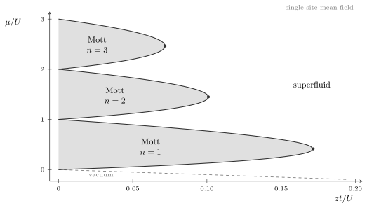
Single-site Gutzwiller mean-field phase boundary for the homogeneous repulsive model. The horizontal axis is $zt/U$, so coordination number is already included. Each shaded lobe has fixed integer filling and zero mean-field order parameter; the surrounding region has $\psi\ne0$. The curves are qualitative in low dimension and are not exact phase boundaries.

What this preview gets right

Single-site mean field correctly organizes the atomic intervals into lobes, identifies the competition between particle and hole fluctuations, and distinguishes incompressible and coherent regimes. It becomes controlled in an appropriate large-coordination limit when hopping is scaled so that $zt$ remains finite.

What it misses

The product state neglects spatial entanglement and long-wavelength fluctuations. It cannot reproduce the one-dimensional Berezinskii–Kosterlitz–Thouless transition, and it gives quantitatively shifted lobe boundaries in finite dimensions.

For example, on the two-dimensional square lattice at unit filling, the single-site prediction is

$$\left(\frac{t}{U}\right)_{\mathrm{tip}}^{\mathrm{MF}} = \frac{(\sqrt2-1)^2}{4} \simeq 0.042893,$$

whereas a high-precision quantum Monte Carlo benchmark gives

$$\left(\frac{t}{U}\right)_{\mathrm{tip}}^{\mathrm{QMC}} = 0.05974(3).$$

This comparison is a warning against treating the schematic lobes as universal data. Cluster mean field, strong-coupling expansions, tensor networks, and quantum Monte Carlo systematically improve different aspects of the problem.

Particle and Hole Motion in a Mott Phase

Finite hopping lets an added particle or hole propagate through the atomic background. On a hypercubic lattice, define

$$\gamma(\mathbf k) = 2 \sum_{\alpha=1}^{d} \cos(k_\alpha a).$$

To first order in $t/U$, the excitation energies above the $n$-particle Mott background are

$$\begin{aligned} E_p(\mathbf k) ={}& Un-\mu -(n+1)t\gamma(\mathbf k) +O(t^2/U), \\ E_h(\mathbf k) ={}& \mu-U(n-1) -nt\gamma(\mathbf k) +O(t^2/U). \end{aligned}$$

The factors $n+1$ and $n$ are Bose-enhanced hopping matrix elements. A particle or hole gap closes at a generic lobe side. Near a commensurate tip, particle and hole sectors become simultaneously important and the long-distance theory acquires an emergent particle–hole symmetry in the standard clean problem.

The detailed critical consequences, including the distinction between $z=2$ side transitions and the standard $z=1$ tip transition, remain in Quantum Phase Transitions.

Weak-Coupling Excitations

In a uniform superfluid, measure the one-particle dispersion from the band bottom:

$$\epsilon_{\mathbf k} = 2t \sum_{\alpha=1}^{d} \left[ 1-\cos(k_\alpha a) \right].$$

A leading lattice Bogoliubov treatment with condensate density $n_0$ gives

$$E_{\mathbf k} = \sqrt{ \epsilon_{\mathbf k} \left( \epsilon_{\mathbf k}+2Un_0 \right) }.$$

At small momentum,

$$E_{\mathbf k} \simeq \hbar c\lvert\mathbf k\rvert, \qquad c = \frac{a}{\hbar} \sqrt{2tUn_0}.$$

This is a weak-depletion result, not a formula for the strongly correlated lobe boundary. The continuum logic and its limitations are introduced in Weakly Interacting Bose Gas Preview.

Optical-Lattice Reduction

An important realization begins with a dilute bosonic field $\hat\Psi(\mathbf r)$ in a periodic optical potential. A standard continuum Hamiltonian is

$$\begin{aligned} H ={}& \int d^3r\, \hat\Psi^\dagger(\mathbf r) \left[ -\frac{\hbar^2\nabla^2}{2m} +V_{\mathrm{lat}}(\mathbf r) +V_{\mathrm{ext}}(\mathbf r) \right] \hat\Psi(\mathbf r) \\ &+ \frac{g}{2} \int d^3r\, \hat\Psi^\dagger(\mathbf r) \hat\Psi^\dagger(\mathbf r) \hat\Psi(\mathbf r) \hat\Psi(\mathbf r). \end{aligned}$$

For a three-dimensional dilute gas away from confinement-induced modifications,

$$g = \frac{4\pi\hbar^2a_s}{m},$$

where $a_s$ is the $s$-wave scattering length.

Lowest-band expansion

If the lowest Bloch band is isolated and relevant energies are small compared with the band gap, expand the field in lowest-band Wannier functions:

$$\hat\Psi(\mathbf r) \simeq \sum_i w_i(\mathbf r)b_i, \qquad w_i(\mathbf r) = w(\mathbf r-\mathbf R_i).$$

Keeping dominant nearest-neighbor hopping and onsite interaction gives the Bose–Hubbard model. The coefficients are

$$\begin{aligned} t_{ij} ={}& - \int d^3r\, w_i^*(\mathbf r) \left[ -\frac{\hbar^2\nabla^2}{2m} +V_{\mathrm{lat}}(\mathbf r) \right] w_j(\mathbf r), \\ U ={}& g \int d^3r\, \lvert w_i(\mathbf r)\rvert^4, \\ \epsilon_i ={}& \int d^3r\, \lvert w_i(\mathbf r)\rvert^2 V_{\mathrm{ext}}(\mathbf r). \end{aligned}$$

These equations explain the model parameters rather than merely naming them. Hopping is an overlap matrix element between neighboring Wannier orbitals. Onsite repulsion is the contact-interaction integral within one localized orbital. A smooth trap appears as a site-dependent energy.

Deep separable lattice

For a separable standing-wave lattice,

$$V_{\mathrm{lat}}(\mathbf r) = \sum_{\alpha} V_\alpha \sin^2(k_\alpha r_\alpha),$$

the recoil energy along one direction is

$$E_R = \frac{\hbar^2k^2}{2m}.$$

For an isotropic deep cubic lattice with $s=V_0/E_R\gg1$, harmonic-Wannier estimates give

$$\frac{t}{E_R} \simeq \frac{4}{\sqrt\pi} s^{3/4}e^{-2\sqrt s},$$

and

$$\frac{U}{E_R} \simeq \sqrt{\frac{8}{\pi}} ka_s s^{3/4}.$$

The hopping falls exponentially with lattice depth, while the onsite interaction changes algebraically in this approximation. Deepening the lattice therefore increases $U/t$ rapidly and can carry the system from a coherent regime toward a Mott regime.

These asymptotic formulas assume a deep, separable lattice, a lowest-band description, weak enough interactions for a single-particle Wannier estimate, and the three-dimensional contact coupling above. They should not be transplanted unchanged to shallow, strongly interacting, low-dimensional, or multiband settings.

Terms discarded by the minimal model

Projection generally also generates smaller terms:

• longer-range hopping;
• offsite density interactions;
• density-assisted tunneling;
• pair hopping;
• coupling to higher bands;
• multibody onsite corrections after orbital deformation.

Their neglect is controlled only when the relevant overlap integrals and virtual-band corrections are small on the energy and time scales of interest.

Validity Checklist

A single-band Bose–Hubbard description is credible when the following questions have quantitative answers:

1. Is the lowest band separated from higher bands by a gap larger than temperature, tunneling, interaction-induced mixing, and drive frequencies?
2. Are longer-range hopping and offsite interactions negligible at the target accuracy?
3. Does one localized orbital per site capture interaction-induced orbital deformation?
4. Are loss and heating slow compared with the dynamics being modeled?
5. Is a spatial trap included explicitly, treated through a local-density approximation, or genuinely negligible?
6. Are the effective parameters calibrated in a convention consistent with the Hamiltonian?

An effective Hamiltonian can be accurate while an assumed equilibrium state is not. Loading through a small many-body gap can create excitations, and a cold initial gas need not remain at the same entropy per particle after the lattice ramp.

Harmonic Traps and Mott Shells

For a slowly varying trap, write

$$K = H_{\mathrm{hom}} + \sum_i \left( V_i-\mu \right)n_i.$$

The local chemical potential is

$$\mu_i = \mu-V_i.$$

Within a local-density approximation, different radii sample different vertical positions in the homogeneous $(t/U,\mu/U)$ diagram. A trapped cloud can therefore contain concentric regions with different integer fillings separated by compressible shells.

This “wedding-cake” structure creates an important distinction: a local Mott plateau can be incompressible even while the total trapped cloud changes size or particle number. A global density response should not be called a homogeneous bulk compressibility without accounting for the trap.

Hard-Core Limit

If repulsion is taken much larger than all other scales and occupations are restricted to

$$n_i\in\{0,1\},$$

the projected operators can be represented by spin-$1/2$ operators:

$$b_i^\dagger \longleftrightarrow S_i^+, \qquad b_i \longleftrightarrow S_i^-, \qquad n_i \longleftrightarrow S_i^z+\frac12.$$

The homogeneous grand Hamiltonian becomes

$$\begin{aligned} K_{\mathrm{hc}} ={}& -2t \sum_{\langle i,j\rangle} \left( S_i^xS_j^x + S_i^yS_j^y \right) \\ &- \mu \sum_i S_i^z + \text{constant}. \end{aligned}$$

The hard-core limit is therefore an $XY$ spin model in a longitudinal field. It is not the same as merely setting $U$ to a large finite number: finite $U$ still permits virtual double occupation and generates corrections. In one dimension, the projected chain can also be mapped to spinless fermions by the Jordan–Wigner transformation.

Finite Systems

A finite lattice has no sharp spontaneous-symmetry-breaking transition. Several diagnostics still expose the approach to the thermodynamic phases:

• avoided crossings and shrinking many-body gaps;
• plateaus in $N(\mu)$ or finite-difference addition energies;
• growth of the largest eigenvalue of $\rho^{(1)}$;
• sensitivity of $E_0$ to a boundary twist;
• changes in onsite number variance and entanglement;
• finite-size scaling of correlation lengths and stiffness.

For canonical energies $E_0(N)$, define the finite-size addition and removal costs

$$\begin{aligned} \mu_+(N) &= E_0(N+1)-E_0(N), \\ \mu_-(N) &= E_0(N)-E_0(N-1). \end{aligned}$$

Their difference

$$\Delta_c(N) = \mu_+(N)-\mu_-(N)$$

is a finite-size charge-gap diagnostic. Its thermodynamic extrapolation, not a single-cluster value, determines whether the bulk is incompressible.

Numerical Representations

Exact diagonalization

At fixed $N$, the basis dimension $\binom{N+L-1}{N}$ grows rapidly but avoids an arbitrary local cutoff. Hopping matrix elements carry square-root factors:

$$b_i^\dagger b_j \lvert\ldots,n_i,\ldots,n_j,\ldots\rangle = \sqrt{(n_i+1)n_j} \lvert\ldots,n_i+1,\ldots,n_j-1,\ldots\rangle.$$

The full sparse-matrix construction lives in Occupation-Number Representation. The Bose–Hubbard Dimer develops the two-site fixed-$N$ blocks and exact observables; its $N=2$ matrix is promoted to the reproducible MB-B005 contract in Benchmark Problems.

Tensor networks

In one dimension, matrix-product-state methods can treat long chains accurately when entanglement and local cutoff are controlled. Near a gapless transition, the bond dimension required for fixed accuracy grows, and finite-entanglement scaling becomes part of the analysis.

Quantum Monte Carlo

The standard unfrustrated repulsive model with real hopping is favorable for worldline and worm algorithms. Complex fluxes, frustration, or additional terms can change that situation. “Bosonic” does not by itself guarantee that every variant is sign-problem free.

Mean-field and cluster methods

Single-site Gutzwiller theory is inexpensive and interpretable, but spatial correlations are absent. Cluster extensions recover short-range entanglement and improve boundaries while retaining a self-consistent environment. Agreement between successive cluster sizes is more informative than a single mean-field curve.

Dimension and Temperature

The zero-temperature phase vocabulary depends on dimension.

• In one dimension, the clean compressible phase is a Luttinger liquid with algebraic one-body correlations. The commensurate lobe tip is a Berezinskii–Kosterlitz–Thouless transition.
• In two dimensions at zero temperature, the superfluid can have true long-range order. At positive temperature, the clean system supports Berezinskii–Kosterlitz–Thouless physics rather than ordinary Bose condensation.
• In three dimensions, a finite-temperature superfluid transition and a normal phase occur above the zero-temperature diagram.

At any positive temperature, an exact zero-temperature Mott gap becomes a crossover scale in thermodynamic observables because thermally activated particles and holes produce nonzero compressibility. A low-temperature state can still display exponentially suppressed compressibility and robust Mott characteristics when

$$k_BT \ll \min(\Delta_p,\Delta_h).$$

Variants

The minimal model is a starting point rather than a universal endpoint.

Variant	Added structure	New possibilities
disordered Bose–Hubbard	random $\epsilon_i$ or $t_{ij}$	Bose glass and Griffiths effects
extended Bose–Hubbard	offsite density interaction	density waves, supersolidity, Haldane-insulator regimes in one dimension
multicomponent model	internal species labels	spin exchange, counterflow, paired phases
flux lattice	complex $t_{ij}$	vortices, frustration, topological bands
driven model	time-dependent coefficients	Floquet engineering, heating, nonequilibrium phases
dissipative model	coupling to reservoirs	nonunitary steady states and loss dynamics
multiband model	several Wannier orbitals per site	orbital physics and interaction-induced band mixing

Each extension changes the Hilbert space, symmetry, and phase diagram. It should be named explicitly rather than folded silently into “the Bose–Hubbard model.”

Common Mistakes

Calling every integer-density state a Mott insulator

Integer average filling is necessary for the standard clean Mott phase but not sufficient. One also needs incompressibility and a finite particle–hole gap in the thermodynamic limit.

Treating a finite-system expectation value as an order parameter

A number eigenstate has $\langle b_i\rangle=0$ even in a finite-size regime that evolves into a superfluid. Use correlation eigenvalues, stiffness, and finite-size scaling.

Equating condensate fraction and superfluid fraction

They coincide in neither definition nor all physical regimes. Low dimension, disorder, and interactions provide important counterexamples.

Forgetting the chemical-potential convention

The phase diagram of $H$ at fixed $N$ and that of $K=H-\mu N$ contain the same canonical energies but organize them differently. Adding $-\mu N$ twice shifts all lobe boundaries incorrectly.

Dropping Bose-enhancement factors

The hopping amplitude between occupation states contains $\sqrt{(n_i+1)n_j}$. Replacing it by $1$ changes both spectra and strong-coupling coefficients.

Reading a mean-field lobe as exact

Single-site mean field is a controlled organizational approximation, not a universal numerical phase diagram. Dimension and lattice geometry matter.

Treating a local cutoff as harmless

A cutoff that is adequate deep in a unit-filling Mott regime can fail badly in a compressible or attractive regime. Convergence must be checked where the occupation distribution is broadest.

Ignoring the optical-lattice validity window

The lowest-band model can fail when interactions mix bands, the lattice is shallow, driving is fast, or neglected tunneling and interaction terms become comparable to the target precision.

Worked Example: Atomic Unit-Filling Window

For $n=1$, the atomic onsite energies are

$$E_0=0, \qquad E_1=-\mu, \qquad E_2=U-2\mu.$$

The one-particle state is lowest when

$$0<\mu<U.$$

Its particle and hole costs are

$$\Delta_p^{(0)} = U-\mu, \qquad \Delta_h^{(0)} = \mu.$$

At $\mu=U/2$, the two costs are equal. This midpoint is particle–hole balanced only in the atomic excitation energies; it is not an exact particle–hole symmetry of the full soft-core model at finite hopping.

Worked Example: Mean-Field Unit-Filling Tip

For $n=1$, the boundary equation becomes

$$y = \frac{x(1-x)}{x+1}.$$

Solving for $x$ gives

$$x_\pm = \frac{1-y}{2} \pm \frac{1}{2} \sqrt{1-6y+y^2}.$$

The tip occurs when the square root vanishes:

$$y^2-6y+1=0.$$

The physical small root is

$$y_{\mathrm{tip}} = 3-2\sqrt2 = (\sqrt2-1)^2.$$

The other root lies outside the small-hopping lobe and is not the relevant branch.

Exercises

Exercise 1: Fixed-number Hilbert space

Derive the number of occupation states for $N$ identical bosons on $L$ sites. Evaluate it for $N=4$ and $L=3$.

Solution

An occupation state is a nonnegative integer solution of

$$n_1+n_2+\cdots+n_L=N.$$

Placing $L-1$ separators among $N$ identical stars gives

$$\dim\mathcal H_{N,L} = \binom{N+L-1}{L-1} = \binom{N+L-1}{N}.$$

For $N=4$ and $L=3$,

$$\dim\mathcal H_{4,3} = \binom{6}{2} =15.$$

Exercise 2: Pair counting

Starting from bosonic ladder operations, prove

$$b^\dagger b^\dagger b b = n(n-1).$$

Solution

Act on an arbitrary number state:

$$bb\lvert n\rangle = \sqrt{n(n-1)} \lvert n-2\rangle.$$

Applying two creation operators returns

$$b^\dagger b^\dagger bb\lvert n\rangle = n(n-1)\lvert n\rangle.$$

Because the number states form a complete basis, the operator identity follows. The eigenvalue counts ordered pairs; the Hamiltonian factor $1/2$ converts this to unordered pairs.

Exercise 3: Atomic occupation interval

Use $E_n=Un(n-1)/2-\mu n$ to determine when $n$ is the onsite ground-state occupation.

Solution

The state $n$ must beat both adjacent occupations. The conditions are

$$E_n<E_{n+1} \quad\Longleftrightarrow\quad \mu<Un,$$

and

$$E_n<E_{n-1} \quad\Longleftrightarrow\quad \mu>U(n-1).$$

Thus

$$U(n-1)<\mu<Un.$$

For a convex onsite spectrum with $U>0$, beating the adjacent levels is sufficient to beat all other occupations.

Exercise 4: Band-bottom mass

Expand the one-dimensional hopping dispersion near $k=0$ and identify the effective mass.

Solution

In one dimension,

$$\varepsilon(k) = -2t\cos(ka).$$

Using $\cos(ka)=1-(ka)^2/2+O(k^4a^4)$,

$$\varepsilon(k) = -2t+ta^2k^2+O(k^4a^4).$$

Matching the energy above the minimum to $\hbar^2k^2/(2m^*)$ gives

$$m^* = \frac{\hbar^2}{2ta^2}.$$

Exercise 5: Mean-field lobe equation

Starting from $r_n=0$, derive the dimensionless boundary

$$y = \frac{(x-n+1)(n-x)}{x+1}.$$

Solution

The condition $r_n=0$ is

$$\frac{1}{zt} = \frac{n}{\mu-U(n-1)} + \frac{n+1}{Un-\mu}.$$

Set $x=\mu/U$ and $y=zt/U$. Then

$$\frac{1}{y} = \frac{n}{x-n+1} + \frac{n+1}{n-x}.$$

Combining fractions gives

$$\frac{1}{y} = \frac{x+1}{(x-n+1)(n-x)}.$$

Inverting yields the stated boundary.

Exercise 6: Locate the mean-field tip

Show that the $n$th lobe tip satisfies

$$\frac{zt}{U} = (\sqrt{n+1}-\sqrt n)^2.$$

Solution

The two branches meet when

$$1-2(2n+1)y+y^2=0.$$

The small root is

$$\begin{aligned} y_{\mathrm{tip}} &= 2n+1-\sqrt{(2n+1)^2-1} \\ &= 2n+1-2\sqrt{n(n+1)} \\ &= (\sqrt{n+1}-\sqrt n)^2. \end{aligned}$$

Substitution into $x=n-1/2-y/2$ gives

$$x_{\mathrm{tip}} = \sqrt{n(n+1)}-1.$$

Exercise 7: Hard-core spin map

Use the hard-core identification to rewrite the hopping term as an $XY$ exchange.

Solution

Within the states $\lvert0\rangle$ and $\lvert1\rangle$,

$$b_i^\dagger b_j+b_j^\dagger b_i \longmapsto S_i^+S_j^-+S_i^-S_j^+.$$

Using $S^\pm=S^x\pm iS^y$,

$$S_i^+S_j^-+S_i^-S_j^+ = 2 \left( S_i^xS_j^x+S_i^yS_j^y \right).$$

Therefore

$$H_t \longmapsto -2t \sum_{\langle i,j\rangle} \left( S_i^xS_j^x+S_i^yS_j^y \right).$$

Exercise 8: Trap routing

A harmonic trap gives $V_i=\tfrac12m\omega^2R_i^2$. Explain why an integer-density plateau near the trap center can coexist with compressible outer shells.

Solution

The local chemical potential is

$$\mu_i = \mu-\frac12m\omega^2R_i^2.$$

It decreases with radius. The center can lie inside a homogeneous Mott lobe, where the local density is pinned and the local compressibility vanishes. Farther out, $\mu_i$ crosses a lobe boundary and samples a compressible superfluid region before eventually entering the vacuum. The whole cloud can therefore change radius or particle number even while its central plateau remains locally incompressible.

Summary

• The Bose–Hubbard model combines bosonic hopping with onsite pair interaction.
• Its soft-core local Hilbert space is infinite, while a fixed-$N$ sector has dimension $\binom{N+L-1}{N}$.
• The atomic limit gives exact integer-filling intervals and particle and hole gaps.
• Hopping broadens those intervals into Mott lobes surrounded by a compressible superfluid.
• Single-site Gutzwiller theory gives an analytic phase-boundary preview but is not quantitatively exact in finite dimension.
• A lowest-band Wannier projection connects the model to bosonic atoms in optical lattices and states the approximation’s validity conditions.
• Compressibility, stiffness, one-body correlations, number fluctuations, and finite-size gaps provide complementary diagnostics.
• The hard-core limit maps to an $XY$ spin model, while attractive and extended variants require separate stability and phase analyses.

Further Reading

• Lattice Models Overview
• Tight-Binding Model
• Bosonic Operators in Many-Body Models
• Occupation-Number Representation
• Bose–Hubbard Dimer
• Bose–Hubbard Chain
• Benchmark Problems
• Momentum-Space Representation
• Grand Canonical Ensemble
• Chemical Potential
• Weakly Interacting Bose Gas Preview
• Quantum Phase Transitions
• Common Many-Body Hamiltonians
• Bose–Hubbard Model Card

References

1. H. A. Gersch and G. C. Knollman, “Quantum Cell Model for Bosons,” Physical Review 129, 959–967 (1963), doi:10.1103/PhysRev.129.959.
2. M. P. A. Fisher, P. B. Weichman, G. Grinstein, and D. S. Fisher, “Boson Localization and the Superfluid-Insulator Transition,” Physical Review B 40, 546–570 (1989), doi:10.1103/PhysRevB.40.546.
3. D. S. Rokhsar and B. G. Kotliar, “Gutzwiller Projection for Bosons,” Physical Review B 44, 10328–10332 (1991), doi:10.1103/PhysRevB.44.10328.
4. K. Sheshadri, H. R. Krishnamurthy, R. Pandit, and T. V. Ramakrishnan, “Superfluid and Insulating Phases in an Interacting-Boson Model: Mean-Field Theory and the RPA,” Europhysics Letters 22, 257–263 (1993), doi:10.1209/0295-5075/22/4/004.
5. D. Jaksch, C. Bruder, J. I. Cirac, C. W. Gardiner, and P. Zoller, “Cold Bosonic Atoms in Optical Lattices,” Physical Review Letters 81, 3108–3111 (1998), doi:10.1103/PhysRevLett.81.3108.
6. D. van Oosten, P. van der Straten, and H. T. C. Stoof, “Quantum Phases in an Optical Lattice,” Physical Review A 63, 053601 (2001), doi:10.1103/PhysRevA.63.053601.
7. M. Greiner, O. Mandel, T. Esslinger, T. W. Hänsch, and I. Bloch, “Quantum Phase Transition from a Superfluid to a Mott Insulator in a Gas of Ultracold Atoms,” Nature 415, 39–44 (2002), doi:10.1038/415039a.
8. W. Zwerger, “Mott–Hubbard Transition of Cold Atoms in Optical Lattices,” Journal of Optics B 5, S9–S16 (2003), doi:10.1088/1464-4266/5/2/352.
9. I. Bloch, J. Dalibard, and W. Zwerger, “Many-Body Physics with Ultracold Gases,” Reviews of Modern Physics 80, 885–964 (2008), doi:10.1103/RevModPhys.80.885.
10. B. Capogrosso-Sansone, Ş. G. Söyler, N. Prokof’ev, and B. Svistunov, “Monte Carlo Study of the Two-Dimensional Bose–Hubbard Model,” Physical Review A 77, 015602 (2008), doi:10.1103/PhysRevA.77.015602.