Variational Many-Body States

A variational many-body state is a restricted, parameterized family of wavefunctions chosen to represent the correlations, symmetries, signs, and entanglement expected in an interacting system. The state family is the physical hypothesis. Optimization decides which member of that family is best for a specified Hamiltonian.

For a nonzero trial state $\lvert\Psi_\theta\rangle$, the variational energy is

$$E(\theta) = \frac{ \langle\Psi_\theta|H|\Psi_\theta\rangle }{ \langle\Psi_\theta|\Psi_\theta\rangle }.$$

If $H$ is self-adjoint and bounded below, then

$$E(\theta) \ge E_0.$$

This inequality is powerful but limited. It certifies an exactly evaluated energy, not the fidelity of every observable, the correctness of an inferred phase, the success of a stochastic optimizer, or the efficiency of representing the state.

The central question is therefore not merely “How many parameters does the ansatz have?” It is:

Which physical structures are easy, hard, or impossible for this state family to express and evaluate?

Canonical Scope

This page is the canonical guide to the structural comparison of important many-body ansätze:

• product and mean-field reference states;
• Slater determinants and determinant expansions;
• Jastrow and other correlator factors;
• BCS, pair-product, and Pfaffian states;
• symmetry and Gutzwiller projection;
• matrix product states as a tensor-network preview;
• neural quantum states as learned amplitude maps;
• hybrid states that combine references, correlators, projections, and flexible representations;
• ansatz selection, evaluation, optimization, and validation criteria.

Neighboring pages retain distinct ownership:

• Variational Principle owns the upper-bound theorem and its spectral proof.
• Trial Wavefunctions owns the general few-body design rules.
• Variational Monte Carlo Preview owns local estimators, sampling error, covariance gradients, and stochastic optimization.
• Slater Determinants owns determinant construction and antisymmetry.
• Hartree–Fock Approximation owns orbital optimization within the single-determinant manifold.
• Reduced BCS Model owns the exact finite-level pairing Hamiltonian and Richardson solution.
• BCS Mean-Field Theory owns the anomalous decoupling, gap equation, coherence factors, and quasiparticles.
• Many-Body Entanglement Overview owns the partition, state-class, measure, and scaling choices needed to compare variational families.
• Entanglement Entropy in Many-Body Systems owns spatial-entanglement scaling and the bond-dimension bound.
• Tensor Networks Preview and Matrix Product States Preview own tensor and MPS structure. DMRG Preview owns finite-system MPS optimization and convergence. Production algorithms remain in the future Computational QM volume.

This page gives enough mathematics to compare the state families without reproducing those canonical derivations.

The Variational Statement in a Many-Body Space

Expand a normalized trial state in exact energy eigenstates:

$$\lvert\Psi_\theta\rangle = \sum_n c_n \lvert n\rangle,$$

where

$$H\lvert n\rangle = E_n\lvert n\rangle, \qquad E_n\ge E_0.$$

Then

$$\begin{aligned} E(\theta)-E_0 &= \sum_n |c_n|^2 \left( E_n-E_0 \right) \\ &\ge 0. \end{aligned}$$

The energy weights errors by excitation energy. A small admixture of a very high-energy state can matter strongly, while substantial rearrangement inside a nearly degenerate low-energy manifold can change observables with little energy penalty.

Sector-resolved upper bounds

If

$$[H,Q] = 0,$$

and the trial state lies entirely in a fixed $Q$ sector, its energy bounds the lowest energy in that sector. This is often the meaningful statement for fixed:

• particle number;
• total momentum;
• parity;
• total spin or a spin component;
• point-group representation;
• topological or gauge-constraint sector.

A trial state in the wrong sector may have a low energy while being irrelevant to the target state.

Stationarity is a projected equation

For a real parameter $\theta_i$,

$$\partial_iE = \frac{ 2\operatorname{Re} \langle \partial_i\Psi_\theta | \left( H-E \right) | \Psi_\theta \rangle }{ \langle\Psi_\theta|\Psi_\theta\rangle }.$$

At a variational stationary point,

$$\langle \partial_i\Psi_\theta | \left( H-E \right) | \Psi_\theta \rangle = 0$$

for every retained tangent direction. The residual need not vanish in the full Hilbert space. It is only orthogonal to the tangent space of the chosen manifold.

Energy variance

For a normalized state, define

$$\sigma_H^2 = \langle H^2\rangle - \langle H\rangle^2.$$

Equivalently,

$$\sigma_H^2 = \left\| \left( H-E \right) \lvert\Psi\rangle \right\|^2.$$

Zero variance means that the state is an exact eigenstate. It does not by itself identify which eigenstate, so energy, symmetry sector, and overlap diagnostics still matter.

Why Many-Body Ansatz Design Is Different

The Scaling of Hilbert Space makes brute-force amplitudes exponentially or combinatorially expensive. A useful ansatz replaces generic coefficients by structure.

That structure should address several independent questions.

Exchange and local constraints

Does the state enforce bosonic or fermionic exchange exactly? Does it remain inside a no-double-occupancy, gauge-invariant, fixed-number, or other constrained Hilbert space?

Sign and phase structure

For fermions and frustrated spins, the difficult information may be the nodes, signs, or complex phases rather than the probability magnitudes. A positive correlator can improve amplitudes without changing nodes.

Correlation range

Short-distance cusps, correlation holes, pairing, density waves, algebraic order, and topological structure require different kinds of nonlocal dependence.

Entanglement structure

A product state has no spatial entanglement. A determinant, paired Gaussian state, projected state, tensor network, and neural state each build entanglement in different ways and with different costs.

Evaluability

The state must support the needed operations:

• amplitude or amplitude-ratio evaluation;
• normalization or expectation-value contraction;
• local-operator matrix elements;
• derivatives with respect to parameters;
• sampling or deterministic summation;
• reduced states or correlators when those observables matter.

An expressive formula whose observables cannot be evaluated at the required scale is not yet a practical variational method.

Optimization geometry

Redundant parameters, gauge freedom, nearly flat directions, sharp curvature, and noisy gradients can make the parameterization much harder to optimize than its parameter count suggests.

Thermodynamic behavior

A state family should be tested for:

• energy extensivity;
• size consistency for separated subsystems;
• stable parameter scaling with system size;
• controlled boundary effects;
• the intended symmetry-breaking or symmetry-restoration limit.

The finite-system variational bound alone does not guarantee any of these.

Taxonomy at a Glance

State family	Structure built in	Main strength	Characteristic limitation
product state	local amplitudes	simple order parameters and limits	no intersite entanglement
Slater determinant	fermionic antisymmetry and exchange	efficient Gaussian observables	one idempotent one-body projector
determinant expansion	linear superposition of references	systematic in a fixed orbital basis	combinatorial determinant count
Jastrow-correlated state	explicit symmetric correlations	cusps and correlation holes	positive factor leaves fermion nodes fixed
BCS or Pfaffian state	pair structure	pairing and anomalous correlations	Gaussian or pair-product bias
Gutzwiller-projected state	local occupancy suppression	constrained correlated fermions	hard expectation values and restricted reference bias
matrix product state	bounded virtual-bond structure	controlled one-dimensional entanglement	bond dimension grows for difficult cuts
neural quantum state	learned amplitude and phase map	flexible nonlocal dependence	nonconvex training and weak a priori control

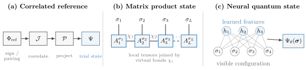
Three complementary architectures. Reference-based states modify a physically motivated $\Phi_{\mathrm{ref}}$ with correlators $\mathcal J$ and projectors $\mathcal P$. Matrix product states factor the coefficient tensor through bonds of dimension $\chi$. Neural quantum states map a configuration $\boldsymbol\sigma$ to a complex amplitude $\Psi_\theta(\boldsymbol\sigma)$.

No row is uniformly “more expressive” in the operational sense. Expressivity depends on the parameter scaling, symmetry sector, target accuracy, observable, and cost allowed for evaluation and optimization.

Product and Mean-Field References

For a lattice with local basis $\{\lvert\sigma_i\rangle\}$, a site-product state is

$$\lvert\Phi_{\mathrm{prod}}\rangle = \bigotimes_{i=1}^{L} \left( \sum_{\sigma_i} f_{i,\sigma_i} \lvert\sigma_i\rangle \right).$$

Such a state can represent:

• classical ordered patterns;
• coherent local moments;
• site-dependent density profiles;
• broken-symmetry mean fields;
• exact product limits of interacting models.

Across every spatial cut,

$$S_A = 0.$$

Product states can display nonzero order parameters, but a pure site-product state has factorized cross-site correlators. Classical mixing can add classical correlations, and projection can turn the reference into a different, correlated state family. Their simplicity makes product states valuable reference points, not generic descriptions of correlated phases.

The phrase Gutzwiller ansatz is used in two different ways:

1. In the Bose–Hubbard literature, a single-site Gutzwiller state is often the product state

   $$\lvert\Psi_{\mathrm{site}}\rangle = \prod_i \sum_n f_{i,n} \lvert n\rangle_i.$$

2. In correlated-fermion work, a Gutzwiller wavefunction usually means a determinant or paired state acted on by a local occupancy projector.

These are not the same ansatz. Bose–Hubbard Model owns the site-product mean-field construction. The fermionic projector is developed below.

Slater Determinants

For $N$ fermions in $N$ orthonormal spin-orbitals, with complete one-particle coordinates $q_i$, a normalized determinant state is

$$\Psi_{\mathrm{SD}} \left( q_1,\ldots,q_N \right) = \frac{1}{\sqrt{N!}} \det \left[ \phi_a(q_i) \right].$$

The determinant:

• enforces antisymmetry exactly;
• vanishes when two identical fermions occupy the same spin-orbital;
• represents a fermionic Gaussian state with fixed particle number;
• permits efficient evaluation of many observables through Wick factorization.

For orthonormal occupied orbitals, its one-body density operator is

$$\gamma = \sum_{a=1}^{N} \lvert\phi_a\rangle \langle\phi_a\rvert,$$

and therefore

$$\gamma^2 = \gamma.$$

The idempotency condition is a structural restriction. An interacting state can have fractional natural-orbital occupations even at zero temperature and cannot then be represented by one determinant.

What a determinant includes

A determinant is not an uncorrelated classical distribution. It contains:

• exact exchange antisymmetry;
• an exchange hole for identical fermions;
• orbital delocalization;
• entanglement associated with a chosen mode or spatial partition.

What it omits is correlation beyond a single Gaussian fixed-number state. Hartree–Fock Approximation optimizes this manifold and owns its direct and exchange fields.

Nodal structure

For a real determinant,

$$D(R) = 0$$

defines its nodes in configuration space. These nodes determine the sign sectors of the wavefunction. Multiplying by a strictly positive scalar factor changes amplitudes inside nodal cells but not the cells themselves.

This distinction matters in fermionic variational and fixed-node Monte Carlo: excellent amplitude correlation cannot repair an incorrect nodal surface unless the ansatz also changes the determinant, uses multiple determinants, backflow, pairing, or another sign-changing structure.

Determinant Expansions

A linear multi-determinant state is

$$\lvert\Psi\rangle = \sum_{I\in\mathcal S} C_I \lvert D_I\rangle.$$

For fixed orbitals and a chosen determinant set $\mathcal S$, optimizing the coefficients is a Rayleigh–Ritz problem. Enlarging $\mathcal S$ cannot increase the exact variational minimum.

Determinant expansions can represent:

• near-degenerate configurations;
• bond breaking and static correlation;
• symmetry-adapted combinations;
• systematic full-configuration-interaction limits in a finite orbital basis.

Their cost grows combinatorially. Truncation by excitation rank, selected configurations, active spaces, or tensor factorization introduces a second modeling choice beyond the one-particle basis.

The phrase “systematic” always needs a qualifier: systematic in which orbital basis, determinant hierarchy, symmetry sector, and extrapolation protocol?

Jastrow Correlators

A Slater–Jastrow state has the form

$$\Psi_{\mathrm{SJ}}(R) = D(R) e^{J(R)},$$

where $R$ denotes the full configuration and $J$ is symmetric under exchange of identical particles. A cluster expansion may be written

$$\begin{aligned} J(R) ={}& \sum_{i<j} u_2(q_i,q_j) \\ &+ \sum_{i<j<k} u_3(q_i,q_j,q_k) + \cdots. \end{aligned}$$

The two-body term can directly encode:

• short-range avoidance;
• interaction cusps;
• screening correlations;
• long-wavelength density fluctuations;
• species- or spin-dependent pair structure.

The three-body and higher terms can distinguish configurations that share the same set of simple pair distances.

Exchange symmetry

If $J(R)$ is symmetric, then

$$e^{J(PR)} = e^{J(R)}$$

for an exchange $P$. Therefore a symmetric Jastrow factor preserves the bosonic or fermionic exchange character of the reference state.

Nodes and phases

If $J$ is real and finite, then

$$e^{J(R)} > 0.$$

Consequently,

$$\Psi_{\mathrm{SJ}}(R) = 0 \quad\Longleftrightarrow\quad D(R) = 0.$$

A positive Jastrow factor does not change fermion nodes. Complex, singular, or sign-changing correlators require a separate analysis and should not be hidden under this statement.

Lattice density Jastrow factor

For lattice occupations, one common form is

$$\mathcal J_n = \exp \left[ - \frac12 \sum_{i,j} v_{ij} \left( n_i-\bar n \right) \left( n_j-\bar n \right) \right].$$

In a translationally invariant system,

$$\mathcal J_n = \exp \left[ - \frac{1}{2L} \sum_{\mathbf q\ne0} v_{\mathbf q} n_{\mathbf q} n_{-\mathbf q} \right],$$

up to the stated Fourier and background conventions.

Short-ranged $v_{ij}$ controls local density correlations. Singular small-$q$ behavior can encode long-range collective suppression. The optimized kernel is state- and Hamiltonian-dependent; calling every density Jastrow “screening” is too vague.

Cusp conditions

For singular interactions, finiteness of the local energy can impose an exact short-distance derivative condition on the wavefunction. A Jastrow factor can build that cusp into the ansatz rather than forcing a large smooth basis to approximate it.

The precise coefficient depends on:

• the interaction normalization;
• reduced mass;
• particle charges or coupling;
• spatial dimension;
• relative angular momentum and spin channel.

The relevant cusp condition should be derived for the Hamiltonian at hand rather than imported by memory.

Evaluation

Jastrow factors make normalization and expectation values genuinely many-body integrals. Cluster expansions work in controlled regimes; otherwise stochastic evaluation is common. Variational Monte Carlo Preview owns the estimator and uncertainty analysis.

Backflow and Nodal Improvement

A backflow state evaluates a determinant at collective coordinates,

$$D(R) \longrightarrow D(X(R)).$$

For a translationally invariant continuum example,

$$\mathbf x_i = \mathbf r_i + \sum_{j\ne i} \eta(r_{ij}) \left( \mathbf r_i-\mathbf r_j \right).$$

Each effective coordinate depends on the surrounding particles. Unlike a positive Jastrow multiplier, backflow generally changes the nodal surface because the determinant zeros are evaluated at $X(R)$ rather than $R$.

Backflow illustrates a general design lesson:

• multiplicative positive correlators improve amplitudes inside sign sectors;
• coordinate transformations and reference superpositions can alter the sign structure itself.

BCS and Pair-Product States

An unprojected spin-singlet BCS state can be written

$$\lvert\mathrm{BCS}\rangle = \prod_{\mathbf k} \left( u_{\mathbf k} + v_{\mathbf k} c_{\mathbf k\uparrow}^\dagger c_{-\mathbf k\downarrow}^\dagger \right) \lvert0\rangle.$$

It is a fermionic Gaussian state in Nambu space. It builds coherent pair structure into the reference but mixes even particle-number sectors.

BCS Mean-Field Theory owns the self-consistent saddle, gap equation, quasiparticles, thermodynamics, and symmetry caveats. Here the important variational fact is that pairing changes the state manifold beyond number-conserving determinants.

Fixed-number pair state

For even $N$, a number-conserving pair-product state can be written schematically as

$$\lvert\Psi_N\rangle \propto \left( \frac12 \sum_{a,b} f_{ab} c_a^\dagger c_b^\dagger \right)^{N/2} \lvert0\rangle,$$

with

$$f_{ab} = -f_{ba}.$$

In a coordinate basis, a general antisymmetric pairing amplitude produces a Pfaffian. For restricted opposite-spin pairing, the amplitude can reduce to a determinant of pair orbitals.

Pair states can express:

• Cooper pairing;
• resonating valence-bond structure after projection;
• spin-triplet or singlet channels;
• richer nodes than a single occupied-orbital determinant.

They remain biased toward pair structure and do not automatically capture every multiparticle correlation.

Particle-number projection

Number projection uses

$$\mathcal P_N = \frac{1}{2\pi} \int_0^{2\pi} d\phi\, e^{i\phi(\widehat N-N)}.$$

Then

$$\lvert\Psi_N\rangle \propto \mathcal P_N \lvert\mathrm{BCS}\rangle$$

has exact particle number. Projection changes expectation values and should not be treated as a cosmetic relabeling of the unprojected saddle.

Symmetry Projection

For a finite group $G$, a projector onto irreducible representation $\alpha$ is

$$\mathcal P_\alpha = \frac{d_\alpha}{|G|} \sum_{g\in G} \chi_\alpha(g)^* U(g),$$

where $d_\alpha$ is the representation dimension and $\chi_\alpha$ its character.

Continuous groups replace the sum by a Haar integral. Projection can restore:

• particle number;
• total momentum;
• point-group quantum numbers;
• parity;
• angular momentum;
• spin quantum numbers.

Projection is especially useful when a simple reference breaks a symmetry whose finite-system eigenstates should preserve it.

Projection after variation and variation after projection

Two procedures differ:

1. Projection after variation: optimize the broken-symmetry reference and project afterward.
2. Variation after projection: evaluate and minimize the projected energy from the start.

The second explores a different energy landscape and is variationally at least as flexible within the projected family, but it is usually more expensive.

If a projector does not commute with another correlator or truncation, the order of operations must be stated.

Fermionic Gutzwiller Projection

For the single-band Hubbard local space, define

$$d_i = n_{i\uparrow} n_{i\downarrow}.$$

A partial Gutzwiller correlator is

$$\mathcal P_{\mathrm G}(g) = \prod_i \left[ 1 - (1-g)d_i \right], \qquad 0\le g\le1.$$

Every doubly occupied site contributes one factor of $g$. Thus:

$$g=1 \quad\Longrightarrow\quad \mathcal P_{\mathrm G}=1,$$

while

$$g=0 \quad\Longrightarrow\quad \mathcal P_{\mathrm G} \text{ removes every doublon.}$$

The Gutzwiller wavefunction is

$$\lvert\Psi_{\mathrm G}\rangle = \mathcal P_{\mathrm G}(g) \lvert\Phi_0\rangle,$$

where $\lvert\Phi_0\rangle$ may be a determinant, density-wave reference, or paired state.

For $0<g<1$, $\mathcal P_{\mathrm G}(g)$ is a correlator but not an idempotent projector:

$$\mathcal P_{\mathrm G}(g)^2 \ne \mathcal P_{\mathrm G}(g).$$

The word “projection” is exact only at the hard endpoints or for an explicitly idempotent constrained-space operator.

What hard projection enforces

At $g=0$,

$$n_{i\uparrow} n_{i\downarrow} \lvert\Psi_{\mathrm G}\rangle = 0$$

for every site. At fixed particle number $N=L$, this also forces one particle per site. Away from half filling, empty sites remain allowed.

The t–J Model Preview owns the no-double-occupancy effective Hamiltonian. A projected variational state respects its local Hilbert space, but that alone does not prove that the chosen reference captures the phase.

Projected BCS and RVB states

A common fixed-number projected pair state is

$$\lvert\Psi_{\mathrm{pBCS}}\rangle \propto \mathcal P_N \mathcal P_{\mathrm G}(0) \lvert\mathrm{BCS}\rangle.$$

At half filling it can be interpreted as a superposition of singlet coverings determined by the pair amplitude. Away from half filling it includes mobile holes in the projected space.

The projection introduces strong non-Gaussian correlations. Wick’s theorem for the unprojected BCS state no longer evaluates projected observables directly.

Worked Example: Hubbard Dimer

Consider two sites, two fermions, and

$$\begin{aligned} H ={}& -t \sum_{\sigma} \left( c_{1\sigma}^\dagger c_{2\sigma} + c_{2\sigma}^\dagger c_{1\sigma} \right) \\ &+ U \sum_{i=1}^{2} n_{i\uparrow}n_{i\downarrow}. \end{aligned}$$

In the even spin-singlet sector, define the covalent and symmetric ionic states

$$\lvert C\rangle = \frac{1}{\sqrt2} \left( c_{1\uparrow}^\dagger c_{2\downarrow}^\dagger - c_{1\downarrow}^\dagger c_{2\uparrow}^\dagger \right) \lvert0\rangle,$$

and

$$\lvert I\rangle = \frac{1}{\sqrt2} \left( c_{1\uparrow}^\dagger c_{1\downarrow}^\dagger + c_{2\uparrow}^\dagger c_{2\downarrow}^\dagger \right) \lvert0\rangle.$$

With a consistent phase convention,

$$H \widehat{=} \begin{pmatrix} 0 & -2t \\ -2t & U \end{pmatrix}$$

in the ordered basis $(\lvert C\rangle,\lvert I\rangle)$.

The noninteracting bonding determinant is

$$\lvert\Phi_0\rangle = \frac{ \lvert C\rangle + \lvert I\rangle }{ \sqrt2 }.$$

Applying the partial Gutzwiller factor gives

$$\lvert\Psi(g)\rangle = \frac{ \lvert C\rangle + g\lvert I\rangle }{ \sqrt{1+g^2} }.$$

Its energy is

$$E(g) = \frac{ Ug^2 - 4tg }{ 1+g^2 }.$$

For $t>0$ and $U\ge0$, stationarity gives

$$2tg^2 + Ug - 2t = 0,$$

so the physical root is

$$g_* = \frac{ \sqrt{U^2+16t^2} - U }{ 4t }.$$

The optimized energy is

$$E(g_*) = \frac{ U - \sqrt{U^2+16t^2} }{ 2 },$$

which is the exact dimer ground-state energy.

This exactness is special: one variational parameter spans every relative mixture of the two basis states in this symmetry sector. The example nevertheless gives three general lessons:

1. At $U=0$, $g_*=1$ and the determinant is exact.

2. At large $U$,

   $$g_* \simeq \frac{2t}{U},$$

   so doublons are suppressed but remain virtually important.

3. Hard projection $g=0$ gives zero energy for this two-site state and misses the finite-$U$ superexchange lowering

   $$E_0 \simeq - \frac{4t^2}{U}.$$

A strict low-energy effective Hamiltonian must retain that virtual process through an exchange term even after doublons are removed from its state space.

Matrix Product States Preview

For an open chain with local basis $\lvert\sigma_i\rangle$, a matrix product state is

$$\begin{aligned} \lvert\Psi\rangle ={}& \sum_{\sigma_1,\ldots,\sigma_L} A_1^{\sigma_1} A_2^{\sigma_2} \cdots A_L^{\sigma_L} \\ &\times \lvert \sigma_1,\ldots,\sigma_L \rangle. \end{aligned}$$

The matrix

$$A_i^{\sigma_i}$$

has dimensions

$$\chi_{i-1} \times \chi_i, \qquad \chi_0=\chi_L=1.$$

The $\chi_i$ are bond dimensions. For approximately uniform local dimension $d$ and bond dimension $\chi$, the raw parameter count scales as

$$O \left( Ld\chi^2 \right),$$

rather than $d^L$.

Entanglement capacity

Across bond $i$, the Schmidt rank is at most $\chi_i$. Therefore

$$S_i \le \ln\chi_i.$$

This makes MPS especially natural for one-dimensional ground states with limited entanglement. It also identifies the failure mode: an exact generic volume-law state requires exponentially large $\chi$.

The entropy bound is necessary, not sufficient. Accuracy also depends on:

• the decay of the Schmidt spectrum;
• the ordering of degrees of freedom along the chain;
• long-range interactions;
• boundary conditions;
• target observables;
• whether the state is critical, highly excited, or time evolved.

Gauge redundancy

On an internal bond, the transformation

$$A_i^{\sigma} \longrightarrow A_i^{\sigma}X,$$

and

$$A_{i+1}^{\sigma'} \longrightarrow X^{-1} A_{i+1}^{\sigma'}$$

leaves the physical coefficients unchanged for invertible $X$.

The tensors are therefore not unique coordinates on state space. Canonical forms organize this gauge freedom and make Schmidt data explicit; their full construction belongs on the dedicated Matrix Product States page.

Exactness and efficiency are different

Every finite-chain state admits an exact MPS if $\chi$ is allowed to grow sufficiently. In the worst case,

$$\chi_{\max} \sim d^{L/2}.$$

Thus “MPS can represent every state” is not an efficiency theorem. The useful statement is that physically important one-dimensional states often admit controlled approximation at much smaller bond dimension.

Neural Quantum States Preview

A neural quantum state uses a parameterized function to assign a complex amplitude to each basis configuration:

$$\Psi_\theta(\boldsymbol\sigma) = \exp \left[ A_\theta(\boldsymbol\sigma) + i\Phi_\theta(\boldsymbol\sigma) \right].$$

Here:

• $A_\theta$ controls the log magnitude;
• $\Phi_\theta$ controls the phase;
• $\boldsymbol\sigma$ may denote spins, occupations, particle coordinates, or another complete configuration.

This logarithmic form is schematic. An exact zero of the amplitude requires a separate vanishing factor or the limiting behavior $A_\theta\to-\infty$.

The architecture is part of the ansatz. Restricted Boltzmann machines, feed-forward networks, convolutional networks, autoregressive models, graph networks, and attention-based models impose different connectivity, symmetry, sampling, and evaluation costs.

Restricted Boltzmann example

For visible spins $s_i=\pm1$ and binary hidden variables summed analytically, a common restricted Boltzmann amplitude is

$$\begin{aligned} \Psi_\theta(\mathbf s) ={}& \exp \left( \sum_i a_is_i \right) \\ &\times \prod_{j=1}^{M} 2\cosh \left( b_j + \sum_i W_{ji}s_i \right). \end{aligned}$$

With real $a_i$, $b_j$, and $W_{ji}$, this expression is positive in the displayed basis. It cannot represent a sign-changing wavefunction. Complex parameters, a separate phase network, a sign-carrying reference state, or another architecture is required.

What neural parameterization can offer

Neural states can encode:

• nonlocal correlations without a fixed geometric tensor network;
• parameter sharing from translation or graph structure;
• separate amplitude and phase models;
• autoregressive conditional amplitudes;
• continuum antisymmetry when combined with determinants or equivariant constructions.

What it does not guarantee

A universal approximation statement may require exponentially many parameters or inaccessible optimization. It does not guarantee:

• efficient training;
• efficient sampling;
• the correct symmetry or sign sector;
• stable local energies;
• accurate observables away from the optimized loss;
• a controlled error as architecture size grows;
• reliable extrapolation in system size.

Neural quantum states are variational ansätze, not a separate variational theorem. Their claims require the same energy, variance, symmetry, finite-size, sampling, and benchmark evidence as traditional states.

Hybrid Ansätze

Useful state families are often composites:

$$\lvert\Psi_\theta\rangle = \mathcal P_{\mathrm{sym}} \mathcal P_{\mathrm G} \mathcal J \lvert\Phi_{\mathrm{pair}}\rangle.$$

Another possibility is

$$\Psi_\theta(R) = D(X_\theta(R)) e^{J_\theta(R)} N_\theta(R),$$

where $N_\theta$ is a symmetric neural correction and $D(X_\theta)$ carries antisymmetry.

Hybrid design lets different factors own different tasks:

Factor	Intended role
determinant or Pfaffian	exchange sign and reference nodes
Jastrow factor	short- and long-range amplitude correlations
backflow	environment-dependent nodal deformation
symmetry projector	exact quantum numbers
Gutzwiller factor	local occupancy suppression
MPS or neural factor	residual structured correlations

The decomposition is not unique. Redundant factors can create ill-conditioned directions, and noncommuting operators make ordering physically relevant.

How to Choose an Ansatz

Start from exact limits

Identify limits in which the state is known:

• noninteracting determinant;
• atomic product state;
• exact dimer or cluster state;
• weak-pairing BCS state;
• no-double-occupancy strong-coupling subspace;
• valence-bond or matrix-product fixed point.

An ansatz that connects smoothly to the relevant limits has an interpretable bias.

Match the hard structure first

Prioritize exact constraints that are difficult to learn numerically:

• exchange antisymmetry;
• particle number;
• local gauge or occupancy constraints;
• boundary conditions;
• known cusps;
• crystal momentum or point-group sector;
• sign rules when established.

Decide what must change

If the reference has:

• good nodes but poor short-range amplitudes, add a Jastrow factor;
• poor nodes, use determinant expansions, pairing, backflow, or a phase-capable model;
• insufficient one-dimensional entanglement, increase MPS bond dimension;
• missing nonlocal structure, add a suitable correlator or architecture;
• broken exact quantum numbers, project or build the symmetry in.

Match evaluation to the state

Determinants and Gaussian states support algebraic contractions. MPS support one-dimensional tensor contractions. Generic Jastrow, projected, and neural states are often evaluated by sampling.

The state and evaluator should be designed together. An ansatz is not fully specified by its amplitude formula alone.

Optimization Error Is Not Ansatz Error

Let

$$E_{\mathcal M} = \inf_{\Psi\in\mathcal M} \frac{ \langle\Psi|H|\Psi\rangle }{ \langle\Psi|\Psi\rangle }$$

be the exact minimum inside ansatz family $\mathcal M$. A reported value can be decomposed schematically as

$$\begin{aligned} E_{\mathrm{reported}}-E_0 ={}& \left( E_{\mathcal M}-E_0 \right) \\ &+ \left( E_{\mathrm{opt}}-E_{\mathcal M} \right) \\ &+ \left( E_{\mathrm{reported}}-E_{\mathrm{opt}} \right). \end{aligned}$$

The terms represent:

1. ansatz error from restricting the state family;
2. optimization error from not finding its minimum;
3. estimation error from finite sampling or approximate contraction.

Only the first two are nonnegative for exact expectation values. A noisy estimate can fall below $E_0$ by chance.

Nonconvex landscapes

Jastrow kernels, projected states, MPS tensors, and neural parameters usually define nonlinear manifolds. Optimization can encounter:

• local minima;
• saddle points;
• symmetry-related solutions;
• gauge directions;
• singular metrics;
• vanishing or noisy gradients;
• phase competition and hysteresis.

Multiple initializations and physically distinct starting states are part of the evidence, not optional cosmetics.

Size Consistency and Extensivity

Suppose two subsystems do not interact:

$$H_{AB} = H_A\otimes I_B + I_A\otimes H_B.$$

If the ansatz can represent

$$\lvert\Psi_{AB}\rangle = \lvert\Psi_A\rangle \otimes \lvert\Psi_B\rangle,$$

then

$$E_{AB} = E_A+E_B.$$

A useful many-body family should recover this separated limit without spurious long-range parameter constraints.

Size consistency can fail when:

• a determinant truncation does not factorize;
• a global correlator retains artificial cross-subsystem terms;
• a projection couples otherwise independent fragments;
• parameter sharing forces inequivalent regions to use the same amplitudes;
• an architecture or normalization changes with total size.

Energy extensivity,

$$E(L) \sim Le_\infty,$$

is related but distinct. Both properties should be checked explicitly.

Observables and Validation

A lower energy is valuable evidence, but it is not enough.

Internal checks

Verify:

• normalization or stable norm ratios;
• exact exchange and symmetry properties;
• local constraints;
• Hermiticity and real energy;
• energy variance;
• convergence with parameter count, bond dimension, determinant count, or network width;
• optimizer and sampling convergence.

Physical checks

Compare:

• local densities and double occupancy;
• pair distributions and cusp behavior;
• one- and two-body density matrices;
• structure factors;
• pairing correlators;
• gaps and response observables;
• entanglement and correlation lengths;
• order parameters with finite-size scaling.

External checks

Use:

• exact limits;
• exact diagonalization on small systems;
• rigorous bounds;
• independent numerical methods;
• known perturbative coefficients;
• sum rules and conservation laws;
• reproducible architecture and optimization sweeps.

Agreement in one observable does not certify the full state.

Common Mistakes

Treating the variational bound as an error bar

$E-E_0$ is unknown unless $E_0$ is independently bounded. The theorem gives a direction, not a numerical uncertainty.

Ranking states only by parameter count

Parameters can be redundant, poorly conditioned, symmetry constrained, or exponentially expensive to evaluate. Structural bias matters more than a raw count.

Calling a positive Jastrow factor a nodal correction

It changes amplitudes but leaves real determinant nodes unchanged.

Calling every occupancy factor a projector

The partial Gutzwiller operator with $0<g<1$ is not idempotent.

Confusing the two Gutzwiller usages

A Bose–Hubbard site-product state and a fermionic no-doublon projector are different constructions.

Assuming hard projection is always optimal at large but finite coupling

Virtual high-energy configurations can lower the energy. An effective Hamiltonian must retain their influence even when its low-energy states exclude them.

Assuming an MPS is efficient because it is exact in principle

Exact representation can require exponentially large bond dimension.

Assuming a neural state learns symmetry or sign automatically

The architecture, parameter domain, reference factor, or explicit projection must support the required sector.

Equating zero variance with the ground state

Every exact eigenstate has zero energy variance.

Using a broken-symmetry finite-system state without qualification

It may approximate local thermodynamic-limit physics while failing to carry the exact finite-system quantum numbers.

Comparing stochastic energies without uncertainty

Autocorrelation, equilibration, heavy tails, and optimization bias can reverse a close ranking.

Optimizing energy and trusting every observable

Nearly degenerate states can have similar energies and very different correlations.

Claiming a phase from one system size

Phase identification requires scaling, competing ansätze, and observables adapted to the proposed order.

Practical Workflow

1. Specify the physical Hilbert space. State statistics, local constraints, particle number, boundary conditions, and basis.
2. Choose the target sector. Record exact and deliberately broken symmetries.
3. Identify exact limits. Determine which reference states should be recovered.
4. Assign structural roles. Decide which factor owns signs, amplitudes, constraints, and entanglement.
5. Choose an evaluator. Establish whether contractions, quadrature, or sampling are feasible.
6. Optimize from distinct starts. Include competing phases and symmetry sectors.
7. Converge the family. Increase determinant count, correlation range, bond dimension, or architecture capacity.
8. Separate errors. Distinguish ansatz, optimization, contraction, and sampling uncertainty.
9. Check physical diagnostics. Do not rely on energy alone.
10. Scale the system. Test extensivity, size consistency, boundaries, and phase diagnostics.
11. Benchmark independently. Use exact limits and another controlled method wherever possible.
12. Report the full state definition. Include conventions, projectors, parameter scaling, optimization protocol, and uncertainty.

Exercises

Spectral upper bound

Let

$$\lvert\Psi\rangle = \sum_n c_n \lvert n\rangle$$

be normalized, with $E_n\ge E_0$. Prove the variational bound and explain when equality holds.

Solution

The energy is

$$E = \sum_n |c_n|^2E_n.$$

Because

$$\sum_n |c_n|^2 = 1,$$

we have

$$\begin{aligned} E-E_0 &= \sum_n |c_n|^2 \left( E_n-E_0 \right) \\ &\ge 0. \end{aligned}$$

Equality requires nonzero coefficients only among states with energy $E_0$. For a nondegenerate ground state, the trial state must equal that ground state up to a phase. For a degenerate ground space, any normalized superposition within that space also saturates the bound.

Jastrow symmetry and nodes

Let $D(R)$ be antisymmetric and let $J(R)$ be a finite real symmetric function. Show that

$$\Psi(R) = D(R)e^{J(R)}$$

is antisymmetric and has exactly the same nodes as $D$.

Solution

For a particle exchange $P$,

$$D(PR) = -D(R),$$

while symmetry gives

$$J(PR) = J(R).$$

Therefore

$$\begin{aligned} \Psi(PR) &= D(PR)e^{J(PR)} \\ &= -D(R)e^{J(R)} \\ &= -\Psi(R). \end{aligned}$$

Because $J$ is finite and real,

$$e^{J(R)} > 0.$$

Hence the product vanishes if and only if $D(R)$ vanishes. The conclusion can fail for a singular, complex, or sign-changing correlator.

Partial Gutzwiller factor

For

$$\mathcal P_{\mathrm G}(g) = \prod_i \left[ 1-(1-g)d_i \right],$$

where $d_i=n_{i\uparrow}n_{i\downarrow}$, show that a basis configuration with $D$ doubly occupied sites acquires weight $g^D$. Determine when $\mathcal P_{\mathrm G}(g)$ is idempotent.

Solution

Since

$$d_i = 0 \quad\text{or}\quad 1$$

on an occupation basis state, the local factor is $1$ on a site without a doublon and $g$ on a doubly occupied site. A configuration with $D$ doublons therefore receives

$$g^D.$$

Applying the operator twice gives $g^{2D}$ rather than $g^D$. Equality for every $D$ requires

$$g^2 = g,$$

so

$$g=0 \quad\text{or}\quad g=1.$$

At $g=0$ the operator projects onto the no-doublon subspace. At $g=1$ it is the identity.

Optimize the Hubbard dimer

Starting from

$$E(g) = \frac{ Ug^2-4tg }{ 1+g^2 },$$

derive the stationary equation and show that the positive root gives the exact ground-state energy.

Solution

Differentiate:

$$\frac{dE}{dg} = \frac{ \left( 2Ug-4t \right) \left( 1+g^2 \right) - 2g \left( Ug^2-4tg \right) }{ \left( 1+g^2 \right)^2 }.$$

The numerator simplifies to

$$2Ug - 4t + 4tg^2.$$

Thus

$$2tg^2 + Ug - 2t = 0.$$

For $t>0$ and $U\ge0$, the physical root is

$$g_* = \frac{ \sqrt{U^2+16t^2} - U }{ 4t }.$$

Substitution gives

$$E(g_*) = \frac{ U-\sqrt{U^2+16t^2} }{ 2 }.$$

This is the lower eigenvalue of

$$\begin{pmatrix} 0 & -2t \\ -2t & U \end{pmatrix}.$$

The variational family is exact here because varying $g$ spans the relative mixture of the two basis vectors in the relevant sector.

MPS entanglement requirement

An open-chain MPS has bond dimension $\chi$ across a cut. Prove that

$$S \le \ln\chi.$$

What scaling of $\chi$ is required by a volume law $S=sL/2$ across the middle of a chain?

Solution

The MPS bond index gives a Schmidt decomposition with at most $\chi$ nonzero Schmidt probabilities. Entropy is maximized when those probabilities are uniform:

$$\lambda_\alpha = \frac{1}{\chi}.$$

Therefore

$$S \le - \sum_{\alpha=1}^{\chi} \frac{1}{\chi} \ln \frac{1}{\chi} = \ln\chi.$$

If

$$S = \frac{sL}{2},$$

then exact representation requires

$$\chi \ge e^S = \exp \left( \frac{sL}{2} \right).$$

The required bond dimension is exponential in system size.

Sign structure of a real RBM

Consider

$$\Psi(\mathbf s) = \exp \left( \sum_i a_is_i \right) \prod_j 2\cosh \left( b_j+\sum_iW_{ji}s_i \right)$$

with all parameters real. Can it represent a basis-dependent wavefunction with both positive and negative amplitudes?

Solution

For real arguments,

$$\exp(x) > 0$$

and

$$\cosh(x) > 0.$$

Every factor is therefore positive, so

$$\Psi(\mathbf s) > 0$$

for every configuration. The displayed real-parameter RBM cannot represent sign changes in that basis. One may use complex parameters, a separate phase model, or multiply by a sign-carrying reference state.

Number projection of BCS

Show that

$$\mathcal P_N = \frac{1}{2\pi} \int_0^{2\pi} d\phi\, e^{i\phi(\widehat N-N)}$$

annihilates every number sector except $N$.

Solution

Let

$$\widehat N \lvert n,\alpha\rangle = n \lvert n,\alpha\rangle.$$

Then

$$\begin{aligned} \mathcal P_N \lvert n,\alpha\rangle &= \frac{1}{2\pi} \int_0^{2\pi} d\phi\, e^{i\phi(n-N)} \lvert n,\alpha\rangle \\ &= \delta_{nN} \lvert n,\alpha\rangle. \end{aligned}$$

The integral is the Fourier orthogonality relation for integer particle number. Applying $\mathcal P_N$ to an unprojected BCS state retains only its $N$-particle component.

Zero variance is not enough

Construct a normalized state with zero energy variance that is not the ground state. What additional information identifies the target?

Solution

Any exact excited eigenstate works. If

$$H\lvert m\rangle = E_m\lvert m\rangle, \qquad E_m>E_0,$$

then

$$\left( H-E_m \right) \lvert m\rangle = 0,$$

so

$$\sigma_H^2 = 0.$$

To identify the ground state one also needs the lowest energy in the relevant symmetry sector or an independent lower bound. For a targeted excited state, one needs its quantum numbers, orthogonality conditions, spectral ordering, or overlap with a known target subspace.

Key Takeaways

• A variational ansatz is a physical restriction on state space, not merely a parameter count.
• Exact exchange, constraints, symmetry, signs, amplitudes, and entanglement are separate design tasks.
• A single determinant is an efficient fermionic Gaussian state with exchange but restricted correlations and nodes.
• A positive symmetric Jastrow factor improves amplitudes without changing determinant nodes.
• BCS and Pfaffian states build pairing into the reference; projection can restore particle number or impose local constraints.
• Partial Gutzwiller factors suppress doublons, while hard projection removes them; these should not be confused with a Bose–Hubbard site-product ansatz.
• MPS efficiency follows from favorable entanglement structure, not from exact representability alone.
• Neural quantum states are flexible ansätze whose symmetry, phase, sampling, optimization, and scaling must be demonstrated.
• Ansatz, optimization, contraction, and sampling errors are logically distinct.
• Energy, variance, observables, system-size scaling, and independent benchmarks all belong in a trustworthy validation.

Cross-Links

• Entanglement Spectrum — Schmidt tails, bond-spectrum extraction, and convergence diagnostics for variational states.

• Volume Laws — extensive cut entropy and the resulting exponential bond-dimension barrier.

• Tensor Networks Preview — the graph, bond, gauge, contraction, and error ledgers behind tensor-network ansätze.

• Matrix Product States Preview — canonical gauges, transfer operators, injectivity, and the MPS–DMRG variational connection.

• DMRG Preview — effective local eigenproblems, finite-system sweeps, Schmidt truncation, and convergence evidence.

• Variational Principle — upper-bound theorem and equality conditions.

• Trial Wavefunctions — general design constraints and limiting behavior.

• Variational Monte Carlo Preview — stochastic expectation values, gradients, variance, and uncertainty.

• First-Quantized Many-Body Wavefunctions — configuration-space amplitudes and exchange symmetry.

• Slater Determinants — determinant construction and normalization.

• Hartree–Fock Approximation — orbital variation in the determinant manifold.

• BCS Mean-Field Theory — pairing saddle, coherence factors, and quasiparticles.

• Entanglement Entropy in Many-Body Systems — area laws and bond-dimension consequences.

• Area Laws — exact MPS and PEPS boundary bounds, Schmidt-tail limitations, and contraction caveats.

• Scaling of Hilbert Space — exact basis-size growth that motivates structured states.

• Hubbard Model — kinetic energy versus local double occupancy.

• t–J Model Preview — hard no-doublon space and projected states.

• Bose–Hubbard Model — site-product Gutzwiller mean field and its distinct terminology.

• Mean-Field Theory — self-consistent reference states, stability, and fluctuations.

References

1. J. C. Slater, “The Theory of Complex Spectra,” Physical Review 34, 1293–1322 (1929), doi:10.1103/PhysRev.34.1293.
2. R. Jastrow, “Many-Body Problem with Strong Forces,” Physical Review 98, 1479–1484 (1955), doi:10.1103/PhysRev.98.1479.
3. J. Bardeen, L. N. Cooper, and J. R. Schrieffer, “Theory of Superconductivity,” Physical Review 108, 1175–1204 (1957), doi:10.1103/PhysRev.108.1175.
4. M. C. Gutzwiller, “Effect of Correlation on the Ferromagnetism of Transition Metals,” Physical Review Letters 10, 159–162 (1963), doi:10.1103/PhysRevLett.10.159.
5. M. C. Gutzwiller, “Effect of Correlation on the Ferromagnetism of Transition Metals,” Physical Review 134, A923–A941 (1964), doi:10.1103/PhysRev.134.A923.
6. P. W. Anderson, “The Resonating Valence Bond State in La2CuO4 and Superconductivity,” Science 235, 1196–1198 (1987), doi:10.1126/science.235.4793.1196.
7. M. Fannes, B. Nachtergaele, and R. F. Werner, “Finitely Correlated States on Quantum Spin Chains,” Communications in Mathematical Physics 144, 443–490 (1992), doi:10.1007/BF02099178.
8. S. Östlund and S. Rommer, “Thermodynamic Limit of Density Matrix Renormalization,” Physical Review Letters 75, 3537–3540 (1995), doi:10.1103/PhysRevLett.75.3537.
9. W. M. C. Foulkes, L. Mitas, R. J. Needs, and G. Rajagopal, “Quantum Monte Carlo Simulations of Solids,” Reviews of Modern Physics 73, 33–83 (2001), doi:10.1103/RevModPhys.73.33.
10. S. Sorella, “Wave Function Optimization in the Variational Monte Carlo Method,” Physical Review B 71, 241103(R) (2005), doi:10.1103/PhysRevB.71.241103.
11. F. Verstraete, V. Murg, and J. I. Cirac, “Matrix Product States, Projected Entangled Pair States, and Variational Renormalization Group Methods for Quantum Spin Systems,” Advances in Physics 57, 143–224 (2008), doi:10.1080/14789940801912366.
12. U. Schollwöck, “The Density-Matrix Renormalization Group in the Age of Matrix Product States,” Annals of Physics 326, 96–192 (2011), doi:10.1016/j.aop.2010.09.012.
13. G. Carleo and M. Troyer, “Solving the Quantum Many-Body Problem with Artificial Neural Networks,” Science 355, 602–606 (2017), doi:10.1126/science.aag2302.
14. G. Carleo, I. Cirac, K. Cranmer, L. Daudet, M. Schuld, N. Tishby, L. Vogt-Maranto, and L. Zdeborová, “Machine Learning and the Physical Sciences,” Reviews of Modern Physics 91, 045002 (2019), doi:10.1103/RevModPhys.91.045002.