Matrix Product States Preview

A matrix product state (MPS) factors the coefficient tensor of a one-dimensional many-body state into an ordered product of matrices. For a chain of $L$ sites with local bases $\{\lvert s_i\rangle\}$,

$$\lvert\psi\rangle = \sum_{s_1,\ldots,s_L} \Psi_{s_1\cdots s_L} \lvert s_1\cdots s_L\rangle,$$

an open-boundary MPS writes

$$\Psi_{s_1\cdots s_L} = A_1^{s_1} A_2^{s_2} \cdots A_L^{s_L},$$

where the right-hand side is a $1\times1$ matrix after all neighboring virtual indices are contracted. More explicitly,

$$\begin{aligned} \Psi_{s_1\cdots s_L} &= \sum_{\alpha_1,\ldots,\alpha_{L-1}} \left(A_1^{s_1}\right)_{\alpha_1} \left(A_2^{s_2}\right)_{\alpha_1\alpha_2} \\ &\quad {}\times\cdots\times \left(A_L^{s_L}\right)_{\alpha_{L-1}}. \end{aligned}$$

The matrix size at bond $i$ is the bond dimension $\chi_i$. It is simultaneously:

• an upper bound on the Schmidt rank across the cut $1\cdots i\vert i+1\cdots L$;
• a coordinate size for the effective left and right boundary spaces;
• a control parameter for representation capacity;
• and, in practical calculations, one of several convergence variables.

It is not an observable and it is not an accuracy certificate by itself.

Scope and Canonical Ownership

This page is the canonical physics-level introduction to MPS as one-dimensional many-body states. It develops:

• finite open and periodic forms;
• site-dependent bond dimensions and parameter scaling;
• the exact relation between MPS bonds and Schmidt decompositions;
• virtual gauge freedom;
• left-, right-, and mixed-canonical forms;
• transfer maps, correlation lengths, injectivity, and parent-Hamiltonian structure;
• representative product, GHZ, and Affleck–Kennedy–Lieb–Tasaki behaviors;
• the conceptual relation between MPS and density-matrix renormalization group;
• symmetry, boundary, ordering, criticality, and dynamics cautions;
• a validation ledger for physical claims made from finite-bond calculations.

Canonical content nearby is deliberately not duplicated:

• Tensor Networks Preview owns the graph dictionary, the comparison among MPS, PEPS, tree networks, and MERA, and general network error accounting.
• Tensor Networks: Computational Guide owns network-family selection, finite-bond convergence design, stopping criteria, and reporting standards.
• Tensor-Network Simulation owns MPS gate updates for circuits, qubit ordering and nonlocal gates, output sampling, spacetime alternatives, and simulator-level resource accounting.
• Entanglement Spectrum owns Schmidt tails, entanglement levels, and discarded-weight interpretation.
• Area Laws owns theorem status and the logical limits of area-law arguments.
• Variational Many-Body States compares MPS with determinant, Jastrow, paired, projected, and neural ansätze.
• Symmetry-Protected Structure Preview owns phase classification and projective-symmetry interpretation.
• The future Computational QM volume owns implementation details: QR and SVD routines, contraction code, tensor data structures, time-evolution kernels, performance scaling, and benchmark notebooks.

The aim here is to understand what an MPS statement means physically and what evidence makes it trustworthy.

Convention Ledger

Unless stated otherwise:

• the chain has sites $i=1,\ldots,L$;
• the local dimension at site $i$ is $q_i$;
• $s_i=1,\ldots,q_i$ is a physical basis label;
• $A_i^{s_i}$ is a $\chi_{i-1}\times\chi_i$ matrix;
• open boundaries mean $\chi_0=\chi_L=1$;
• $\chi=\max_i\chi_i$ denotes a typical or maximum bond dimension;
• $\bar A$ denotes the complex conjugate of $A$ in the declared basis;
• $\dagger$ denotes Hermitian conjugation;
• states are normalized unless an unnormalized form is explicitly being discussed;
• logarithms are natural, so entropies are in nats.

The ordering of sites is part of the representation. A permutation of orbitals or lattice sites is a physical relabeling of the tensor factors but can change every intermediate Schmidt rank and therefore the MPS cost.

Exact, approximate, and optimized

Three statements must be separated:

1. An exact MPS reproduces every amplitude of the target finite state.
2. An approximate MPS is close under a declared state, observable, or reduced-state metric.
3. An optimized MPS is the output of a specified search procedure within a chosen MPS manifold.

An optimized state need not be the best state at that bond dimension. The best state at that bond dimension need not be accurate for the physical question. Exact representability at some unrestricted bond dimension does not imply efficiency.

Open-Boundary MPS

For open boundaries, the tensor at site $i$ has components

$$\begin{gathered} \left(A_i^{s_i}\right)_{\alpha_{i-1}\alpha_i}, \\ \alpha_{i-1}=1,\ldots,\chi_{i-1}, \\ \alpha_i=1,\ldots,\chi_i. \end{gathered}$$

The endpoint tensors are a row and a column:

$$A_1^{s_1} \in \mathbb C^{1\times\chi_1}, \qquad A_L^{s_L} \in \mathbb C^{\chi_{L-1}\times1}.$$

One may instead use square bulk matrices and explicit boundary vectors,

$$\Psi_{s_1\cdots s_L} = \ell^\dagger A_1^{s_1}\cdots A_L^{s_L} r.$$

These conventions are equivalent after absorbing $\ell^\dagger$ and $r$ into the endpoint tensors. A derivation should state which convention it uses because dimensions and gauge transformations at the boundaries differ.

Raw parameter count

Before accounting for gauge redundancy, an open MPS contains

$$N_{\mathrm{raw}} = \sum_{i=1}^{L} q_i\chi_{i-1}\chi_i$$

complex tensor entries. For uniform $q_i=q$ and interior $\chi_i=\chi$,

$$N_{\mathrm{raw}} = O(Lq\chi^2).$$

This should be compared with the generic coefficient count

$$\prod_{i=1}^{L}q_i,$$

which is $q^L$ for a uniform chain. Polynomial storage follows only when a physically adequate $\chi$ remains polynomial in $L$ and the desired precision.

Nonuniform bond dimensions are natural

The maximum possible Schmidt rank depends on the cut:

$$\chi_i^{\max} = \min \left( \prod_{j=1}^{i}q_j, \prod_{j=i+1}^{L}q_j \right).$$

Near an open edge this ceiling is small. Near the center it can be exponentially large. Padding every bond to one common $\chi$ is convenient notation, not a structural requirement.

For a uniform chain,

$$\chi_i^{\max} = q^{\min(i,L-i)}.$$

A generic state approaches this ceiling near the middle. The statement that every finite chain state has an exact MPS is therefore true but computationally weak.

Periodic-Boundary MPS

A common periodic form is

$$\Psi_{s_1\cdots s_L} = \operatorname{Tr} \left( A_1^{s_1} A_2^{s_2} \cdots A_L^{s_L} \right),$$

where all matrices close into a loop. For a translation-invariant representation one may set

$$A_i^s=A^s,$$

although a translation-invariant state need not be most conveniently represented by a one-site tensor before blocking or gauge adjustment.

A contiguous bipartition of a periodic ring cuts two virtual bonds. If both have dimension $\chi$, then

$$\operatorname{SchmidtRank}_A \le \chi^2, \qquad S_A \le 2\ln\chi.$$

Open- and periodic-boundary bond dimensions should therefore not be compared without specifying the cut geometry. Periodic MPS also have less favorable contraction and canonicalization structure; those algorithmic details belong in Computational QM.

Bonds and Schmidt Decompositions

Consider the cut after site $i$:

$$\mathcal H = \mathcal H_{1\cdots i} \otimes \mathcal H_{i+1\cdots L}.$$

Contracting all tensors left of the cut defines at most $\chi_i$ left vectors,

$$\lvert\widetilde L_{\alpha}\rangle, \qquad \alpha=1,\ldots,\chi_i,$$

and contracting the right side defines at most $\chi_i$ right vectors,

$$\lvert\widetilde R_{\alpha}\rangle.$$

Thus the state can be written

$$\lvert\psi\rangle = \sum_{\alpha=1}^{\chi_i} \lvert\widetilde L_\alpha\rangle \lvert\widetilde R_\alpha\rangle,$$

so

$$\operatorname{SchmidtRank}_{1\cdots i\vert i+1\cdots L} \le \chi_i.$$

After orthonormalizing the two block bases, the same cut takes Schmidt form:

$$\lvert\psi\rangle = \sum_{\alpha=1}^{r_i} \lambda_\alpha^{[i]} \lvert L_\alpha^{[i]}\rangle \lvert R_\alpha^{[i]}\rangle,$$

with

$$\lambda_\alpha^{[i]}\ge0, \qquad \sum_{\alpha=1}^{r_i} \left(\lambda_\alpha^{[i]}\right)^2 =1, \qquad r_i\le\chi_i.$$

If zero-padding is removed, the minimum exact bond dimension at that cut is precisely $r_i$.

Entropy capacity

The reduced-state eigenvalues are

$$p_\alpha^{[i]} = \left(\lambda_\alpha^{[i]}\right)^2.$$

Therefore

$$S_i = -\sum_{\alpha=1}^{r_i} p_\alpha^{[i]} \ln p_\alpha^{[i]} \le \ln r_i \le \ln\chi_i.$$

Every Rényi entropy of positive order obeys the same rank ceiling:

$$S_n^{[i]} \le \ln\chi_i, \qquad n>0.$$

Consequently, a target cut entropy $S_i$ requires

$$\chi_i \ge e^{S_i}.$$

This is a necessary capacity condition, not a sufficient approximation theorem. Entropy does not determine how quickly the Schmidt tail decays.

Truncation at one cut

Keeping the largest $\chi$ Schmidt values gives the unnormalized vector

$$\lvert\widetilde\psi_\chi\rangle = \sum_{\alpha=1}^{\chi} \lambda_\alpha \lvert L_\alpha\rangle \lvert R_\alpha\rangle.$$

Its squared norm is

$$\langle\widetilde\psi_\chi \vert \widetilde\psi_\chi\rangle = 1-\epsilon_\chi,$$

where

$$\epsilon_\chi = \sum_{\alpha>\chi} \lambda_\alpha^2$$

is the discarded weight at that cut. The normalized truncated state has fidelity

$$\left| \langle\psi\vert\psi_\chi\rangle \right|^2 = 1-\epsilon_\chi.$$

Sequential truncations across many cuts do not generally combine into one global error by simply quoting the largest local discarded weight. The Entanglement Spectrum page owns the detailed tail and truncation ledger.

Virtual Gauge Freedom

MPS tensors are coordinates, not observables. On an interior bond, insert an invertible matrix and its inverse:

$$X_iX_i^{-1} = I_{\chi_i}.$$

The transformations

$$A_i^{s_i} \longmapsto A_i^{s_i}X_i, \qquad A_{i+1}^{s_{i+1}} \longmapsto X_i^{-1}A_{i+1}^{s_{i+1}}$$

leave every physical amplitude unchanged. More generally,

$$A_i^{s_i} \longmapsto X_{i-1}^{-1} A_i^{s_i} X_i,$$

with the endpoint convention adjusted appropriately.

Consequences

Gauge freedom means:

• tensor entries are not directly physical;
• norms can migrate from one tensor to another;
• raw differences between two tensor files are meaningless before gauge alignment;
• optimization may contain flat or poorly conditioned coordinate directions;
• canonical gauges can expose orthonormal block bases and Schmidt data;
• gauge-invariant observables, transfer spectra, and Schmidt values are the appropriate comparison objects.

This virtual basis redundancy is not a physical gauge symmetry. A Gauss-law constraint restricts the physical Hilbert space; an MPS gauge change only rewrites the same vector.

Singular bonds

The transformation matrices must be invertible on the represented bond support. If a bond contains zero Schmidt values or deliberately padded null directions, the full $\chi_i\times\chi_i$ gauge is not unique in the same way. Canonicalization should first identify the supported subspace rather than treating null directions as physical degeneracy.

Canonical Forms

Canonical forms use gauge freedom to make the effective block states orthonormal. They are especially powerful for open chains because removing one bond disconnects the graph.

Left-canonical tensors

With $A_{L,i}^s$ viewed as a matrix from the left bond to the right bond, the left-canonical condition is

$$\sum_s \left(A_{L,i}^{s}\right)^\dagger A_{L,i}^{s} = I_{\chi_i}.$$

Equivalently, reshape the tensor into a matrix whose row index is $(\alpha_{i-1},s)$ and whose column index is $\alpha_i$. Its columns are orthonormal.

If all tensors through site $i$ are left-canonical, the recursively constructed states

$$\begin{aligned} \lvert L_{\alpha_i}^{[i]}\rangle &= \sum_{\substack{ s_1,\ldots,s_i\\ \alpha_1,\ldots,\alpha_{i-1} }} \\ &\quad {}\times \left( A_{L,1}^{s_1} \cdots A_{L,i}^{s_i} \right)_{\alpha_i} \lvert s_1\cdots s_i\rangle. \end{aligned}$$

satisfy

$$\left\langle L_{\alpha_i}^{[i]} \middle| L_{\beta_i}^{[i]} \right\rangle = \delta_{\alpha_i\beta_i}.$$

The proof is inductive: contraction of the newest physical index applies the left-canonical identity and preserves orthonormality.

Right-canonical tensors

The right-canonical condition is

$$\sum_s A_{R,i}^{s} \left(A_{R,i}^{s}\right)^\dagger = I_{\chi_{i-1}}.$$

Tensors from site $i$ to the right boundary then generate orthonormal right-block states.

Mixed-canonical form

Choose a cut after site $i$. Tensors to the left can be left-canonical and tensors to the right right-canonical, leaving a diagonal center matrix

$$\Lambda^{[i]} = \operatorname{diag} \left( \lambda_1^{[i]}, \ldots, \lambda_{r_i}^{[i]} \right).$$

The state becomes

$$\lvert\psi\rangle = \sum_{\alpha=1}^{r_i} \lambda_\alpha^{[i]} \lvert L_\alpha^{[i]}\rangle \lvert R_\alpha^{[i]}\rangle.$$

Thus a mixed-canonical MPS is the Schmidt decomposition written locally along a chain.

One may instead place the orthogonality center on a site, represented by a center tensor $A_{C,i}^s$. In a compatible gauge,

$$A_{C,i}^s = A_{L,i}^s C_i = C_{i-1}A_{R,i}^s.$$

The matrices $C_i$ need not be diagonal in every working gauge, but their singular values are the Schmidt values across the corresponding bond.

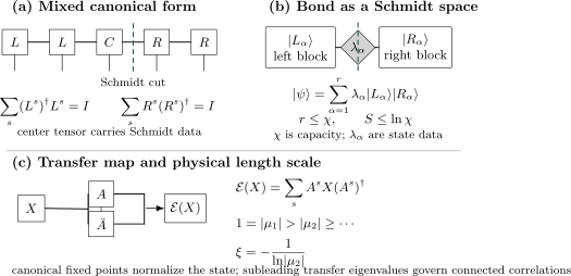
Three complementary views of an MPS. Left- and right-canonical tensors generate orthonormal block bases around a center. The center bond carries Schmidt values $\lambda_\alpha$, with rank $r\le\chi$ and entropy $S\le\ln\chi$. For a uniform MPS, the transfer map $\mathcal E$ fixes normalization and its subleading eigenvalues set correlation scales.

Why canonical form is useful

In mixed-canonical form:

• the norm is a local contraction of the center data;
• Schmidt values and entanglement entropy are directly available;
• expectation-value environments are well conditioned;
• the meaningful support of a bond is visible;
• truncation can be defined by ordered Schmidt values;
• local optimization has a transparent effective basis.

Canonical form does not make the physical state unique. Degenerate Schmidt values permit unitary rotations within degenerate sectors, phases remain, and null directions remain arbitrary.

Moving the center does not change the state

Shifting an orthogonality center by one site amounts to factorizing the current center tensor and absorbing one factor into its neighbor. At the exact algebraic level this is a gauge change. If singular values are discarded during the move, it becomes an approximation.

This distinction is fundamental:

$$\begin{gathered} \text{exact center move} \\ \neq \\ \text{truncating center move}. \end{gathered}$$

The numerical QR and SVD procedures used to carry out these operations belong in the future Computational QM implementation page.

Transfer Maps and Contractions

For a uniform MPS with square $\chi\times\chi$ matrices $A^s$, define the transfer map

$$\mathcal E(X) = \sum_s A^sX(A^s)^\dagger.$$

Its Hilbert–Schmidt adjoint is

$$\mathcal E^\ast(Y) = \sum_s (A^s)^\dagger Y A^s.$$

The right-canonical condition gives

$$\mathcal E(I)=I,$$

whereas the left-canonical condition gives

$$\mathcal E^\ast(I)=I.$$

For a generic canonical uniform MPS, one works with positive left and right fixed points,

$$\mathcal E(r)=r, \qquad \mathcal E^\ast(\ell)=\ell,$$

normalized by

$$\operatorname{Tr}(\ell r)=1.$$

Gauge transformations move information between $A$, $\ell$, and $r$ without changing physical contractions.

Norm as repeated transfer

For boundary matrices $\ell_0$ and $r_L$, the norm of a length-$L$ uniform chain is a contraction of repeated transfer maps:

$$\langle\psi\vert\psi\rangle = \operatorname{Tr} \left[ \ell_0\, \mathcal E^L(r_L) \right],$$

up to the chosen placement of adjoints and boundary-vector convention. The important structural fact is that the exponentially large physical sum is replaced by iteration on a $\chi^2$-dimensional virtual operator space.

For a site-dependent MPS, use

$$\mathcal E_i(X) = \sum_{s_i} A_i^{s_i} X \left(A_i^{s_i}\right)^\dagger$$

with dimensions adjusted from bond to bond.

Operator insertion

A local operator $O$ is inserted through

$$\mathcal E_O(X) = \sum_{s,s'} \langle s'\lvert O\rvert s\rangle A^sX(A^{s'})^\dagger.$$

Products of transfer maps and inserted maps generate expectation values and correlation functions. This is why MPS observables can be evaluated without explicitly forming the $q^L$ amplitudes.

An efficient representation and an efficient contraction are distinct claims in general tensor networks. For an open MPS, the loop-free chain geometry makes standard norm and local-observable contractions polynomial in $L$, $q$, and $\chi$.

Transfer Spectrum and Correlations

Let the transfer map be normalized so its spectral radius is one. Denote its eigenvalues by

$$\mu_0=1, \qquad \lvert\mu_1\rvert \ge \lvert\mu_2\rvert \ge \cdots.$$

When the leading eigenvalue is unique and the relevant subleading eigenvalues satisfy

$$\lvert\mu_a\rvert<1,$$

a connected two-point function at separation $r$ has the schematic form

$$\langle O_0P_r\rangle_c = \sum_{a\ge1} c_a(O,P)\, \mu_a^{\,r-1},$$

with possible polynomial prefactors if the transfer map has nontrivial Jordan blocks.

The largest contributing magnitude defines a correlation length

$$\xi_{O,P} = -\frac1{ \ln\lvert\mu_{\mathrm{lead}}(O,P)\rvert }.$$

A commonly quoted transfer correlation length is

$$\xi = -\frac1{\ln\lvert\mu_1\rvert},$$

provided $\mu_1$ couples to some local operators and the leading fixed point is nondegenerate.

What the transfer spectrum does not prove

A finite transfer correlation length of one converged MPS does not by itself prove a spectral gap of the Hamiltonian. It may reflect:

• a genuinely gapped phase;
• finite bond dimension near a critical point;
• finite system size;
• explicit symmetry breaking in the selected state;
• a metastable optimization result;
• a state-ordering or boundary artifact.

Physical claims require convergence in $\chi$ and $L$, symmetry and boundary checks, and direct spectral or scaling evidence where appropriate.

Degenerate leading eigenvalues

If several transfer eigenvalues have magnitude one, the state may contain persistent order, symmetry-broken sectors, periodic structure, or non-injective blocks. The bond-dimension-two GHZ representation on Tensor Networks Preview is the simplest warning: its entropy is bounded, yet a connected $Z$ correlator does not decay.

Low entanglement therefore does not imply clustering without additional structure.

Injectivity

For a uniform MPS, block $\ell$ sites and define the map

$$\begin{aligned} \Gamma_\ell(X) &= \sum_{s_1,\ldots,s_\ell} \\ &\quad {}\times \operatorname{Tr} \left( X A^{s_1}\cdots A^{s_\ell} \right) \lvert s_1\cdots s_\ell\rangle. \end{aligned}$$

The MPS is injective after $\ell$ sites if

$$\Gamma_\ell(X)=0 \quad\Longrightarrow\quad X=0.$$

Equivalently, after a sufficiently large finite blocking, products

$$A^{s_1}\cdots A^{s_\ell}$$

span the full virtual matrix algebra.

Injectivity is a structural condition, not a synonym for finite bond dimension. A finite-$\chi$ MPS can be non-injective.

Consequences under standard assumptions

For an injective uniform MPS:

• the canonical transfer map has a unique full-rank fixed-point structure;
• connected correlations cluster exponentially;
• sufficiently long local reduced states determine a frustration-free parent Hamiltonian;
• the periodic parent Hamiltonian has the MPS as a unique ground state for sufficiently large rings;
• the associated parent-Hamiltonian family is gapped under the standard finite-range construction.

The precise blocking length, interaction range, and finite-size qualifications matter. These statements concern the constructed parent Hamiltonian, not every Hamiltonian for which the MPS happens to approximate a low-energy state.

Parent Hamiltonian construction

Choose a block length $\ell$ for which the MPS reduced state has support

$$\mathcal S_\ell \subseteq \bigotimes_{j=1}^{\ell} \mathcal H_j.$$

Let

$$h_i$$

be the projector onto the orthogonal complement of that support on sites $i,\ldots,i+\ell-1$. Then

$$H_{\mathrm{parent}} = \sum_i h_i$$

is positive semidefinite and

$$H_{\mathrm{parent}}\lvert\psi\rangle=0.$$

Hence the MPS is an exact frustration-free ground state. Injectivity supplies the strong uniqueness and stability properties; without it, the parent ground space can be degenerate.

Non-injective structure

Non-injective MPS are not defective. They naturally describe:

• cat states and symmetry-breaking sectors;
• states with periodicity larger than the chosen unit cell;
• degenerate parent-Hamiltonian ground spaces;
• block structures carrying distinct superselection-like sectors.

The correct response is to identify the block structure and physical sector, not to force a single injective interpretation.

Finite, Uniform, and Infinite MPS

The phrase “an MPS” can refer to several distinct limits.

Form	Tensors	Boundary data	Typical use
finite open MPS	site dependent or uniform	endpoint tensors or vectors	finite chains, edge states, DMRG
finite periodic MPS	loop of tensors	trace or closure tensor	rings and translation studies
uniform infinite MPS	one repeating tensor or unit cell	transfer fixed points	thermodynamic-limit phases
finite MPS on a cylinder path	ordered 2D sites mapped to a chain	open or infinite along the axis	quasi-one-dimensional systems

These forms have different cut counts, boundary physics, and convergence questions.

Translation invariance

Using one repeated tensor makes translation invariance manifest, but the converse needs care. A translation-invariant physical state may require:

• a larger unit cell in the chosen representation;
• blocking before injectivity appears;
• a superposition of symmetry-broken blocks;
• boundary data that restore a finite-ring symmetry.

One should distinguish a symmetry of the state from a symmetry of a particular tensor gauge.

Thermodynamic normalization

For an infinite uniform MPS, the global vector norm is not formed by taking an ordinary finite trace at $L=\infty$. Local expectation values are defined through normalized transfer fixed points. A well-posed statement specifies the unit cell, fixed-point normalization, and selected sector.

Boundary Conditions and Site Ordering

MPS geometry follows an ordered path. That path need not coincide with Euclidean distance.

Open edges

Open boundary vectors can:

• select a state within a degenerate parent ground space;
• expose edge degrees of freedom;
• break or preserve a symmetry;
• change one-point functions near the boundary;
• leave bulk transfer properties unchanged in a sufficiently long injective chain.

Bulk conclusions should be separated from edge conclusions and checked as the observation point moves away from the endpoints.

Periodic rings

A periodic ring removes physical edges but introduces a loop in the contraction. A contiguous region has two virtual boundaries, so its rank capacity is $\chi^2$, not $\chi$. Finite-ring momentum and translation quantum numbers also depend on how the trace and unit cell are implemented.

Use Boundary Conditions on Lattices for the canonical boundary-condition ledger.

Ladders and cylinders

A ladder or cylinder can be mapped to a one-dimensional ordering, but a cut across the MPS path may cross a physical boundary whose size grows with the transverse width $W$. An area-law state can then require

$$\ln\chi = O(W),$$

or

$$\chi = e^{O(W)}.$$

MPS methods can still be powerful for narrow cylinders, but “area law” does not mean cost independent of width.

Orbital ordering

For quantum chemistry, long-range spin models, or momentum-space problems, the site order may be a design choice. Two orderings represent the same physical tensor product but can have very different cut entropies. A trustworthy comparison states the ordering and checks whether the conclusion is stable under plausible alternatives.

Representative MPS Structures

Product states

Bond dimension one gives

$$A_i^{s_i}=a_i^{s_i},$$

so the amplitude factorizes and the state is a product. This is the zero-entanglement baseline.

The full coefficient check is developed on Tensor Networks Preview; here the structural point is

$$\chi_i=1 \quad\Longleftrightarrow\quad r_i=1$$

at every cut for a pure finite-chain state.

GHZ states

The GHZ state has an exact $\chi=2$ MPS, constant cut entropy $\ln2$, and nondecaying order. Its transfer map has more than one leading sector. It is therefore a compact but non-injective counterexample to the claim that finite bond dimension forces short-range correlations.

The Affleck–Kennedy–Lieb–Tasaki state

The spin-1 Affleck–Kennedy–Lieb–Tasaki (AKLT) state is a canonical example of a nontrivial gapped MPS. In the physical basis

$$\lvert+\rangle, \qquad \lvert0\rangle, \qquad \lvert-\rangle,$$

one convenient bond-dimension-two representation is

$$\begin{aligned} A^+ &= \sqrt{\frac23}\, \sigma^+, \\ A^0 &= -\frac1{\sqrt3}\, \sigma^z, \\ A^- &= -\sqrt{\frac23}\, \sigma^-. \end{aligned}$$

With

$$\sigma^+ = \begin{pmatrix} 0&1 \\ 0&0 \end{pmatrix}, \qquad \sigma^- = \begin{pmatrix} 0&0 \\ 1&0 \end{pmatrix},$$

these tensors obey both canonical identities:

$$\sum_{m=+,0,-} (A^m)^\dagger A^m = I,$$

and

$$\sum_{m=+,0,-} A^m(A^m)^\dagger = I.$$

The transfer map has eigenvalue

$$\mu_0=1$$

on the identity sector and

$$\mu_x=\mu_y=\mu_z=-\frac13$$

on the Pauli sector. Hence the bulk correlation length is

$$\xi_{\mathrm{AKLT}} = \frac1{\ln3}.$$

The sign produces staggered correlations, while the magnitude gives exponential decay.

The corresponding nearest-neighbor parent Hamiltonian can be written

$$H_{\mathrm{AKLT}} = 2\sum_i P_{i,i+1}^{(S=2)},$$

or equivalently

$$\begin{aligned} H_{\mathrm{AKLT}} = \sum_i \Bigg[ &\mathbf S_i\cdot\mathbf S_{i+1} \\ &+ \frac13 \left( \mathbf S_i\cdot\mathbf S_{i+1} \right)^2 + \frac23 \Bigg]. \end{aligned}$$

Every term annihilates the valence-bond-solid state. On an open chain, unpaired virtual spin-$1/2$ edge degrees of freedom produce boundary-state structure. On a periodic chain, the injective bulk MPS gives a unique ground state for the standard sufficiently large ring.

Across a bulk cut of the infinite canonical state, the two Schmidt probabilities are equal:

$$p_1=p_2=\frac12,$$

so

$$S=\ln2.$$

This one example ties together bond dimension, canonical gauge, transfer spectrum, exponential clustering, edge structure, and a frustration-free parent Hamiltonian.

Symmetries on Physical and Virtual Indices

Suppose an on-site unitary symmetry acts as

$$U_g = u_g^{\otimes L}.$$

For an injective uniform MPS invariant up to a phase, the local tensors satisfy a relation of the form

$$\sum_{s'} (u_g)_{ss'} A^{s'} = e^{i\theta_g} V_g^{-1} A^s V_g.$$

The physical action can therefore be pushed to the virtual bonds. The matrices $V_g$ may form a projective representation,

$$V_gV_h = \omega(g,h) V_{gh}.$$

Under the appropriate symmetry and gap assumptions, the cohomology class of $\omega(g,h)$ carries symmetry-protected phase information. The Symmetry-Protected Structure Preview page owns that classification.

Symmetry-resolved bonds

In a symmetry-adapted MPS, bond spaces decompose into charge sectors:

$$\mathcal V_i = \bigoplus_Q \mathcal V_{i,Q}.$$

Tensor blocks vanish unless the incoming bond charge, physical charge, and outgoing bond charge satisfy the declared fusion rule. For an Abelian additive convention,

$$Q_{\mathrm{left}}+q_s = Q_{\mathrm{right}}.$$

Benefits include:

• exact conservation of selected quantum numbers;
• block-sparse storage and contraction;
• symmetry-resolved Schmidt spectra;
• cleaner targeting of physical sectors.

The charge convention and degeneracy spaces must be documented. A block-sparse tensor is not evidence that the intended global symmetry sector was selected correctly.

Fermions

A fermionic MPS needs an explicit parity and ordering convention. One may use Jordan–Wigner strings, parity-aware tensor categories, or a fermionic swap rule. Omitting the convention makes sign-sensitive formulas ambiguous even if the drawn network looks identical to a spin MPS.

Why MPS and DMRG Fit Together

Density-matrix renormalization group (DMRG) is naturally understood as variational optimization over MPS. At fixed bond dimensions, one seeks

$$E_{\min} = \min_{\lvert\psi(A)\rangle\in\mathcal M_{\{\chi_i\}}} \frac{ \langle\psi(A)\lvert H\rvert\psi(A)\rangle }{ \langle\psi(A)\vert\psi(A)\rangle },$$

where

$$\mathcal M_{\{\chi_i\}}$$

is the MPS manifold with the chosen boundary conditions, local spaces, symmetries, and bond profile.

Canonical form supplies orthonormal effective block bases around a local center. DMRG then updates local center data while holding an environment fixed, moves the center, and repeats. The density-matrix language and the MPS language meet at the Schmidt decomposition: retaining dominant reduced-state eigenvectors is retaining dominant bond Schmidt sectors.

Why one-dimensional gapped systems are favorable

Broad classes of one-dimensional finite-range gapped ground states obey area laws and admit controlled MPS approximations. Locality, a stable gap, and favorable Schmidt tails make moderate bond dimensions physically effective.

The logical chain is not

$$\begin{gathered} \text{gapped} \\ \not\Longrightarrow \\ \text{small fixed }\chi \\ \text{for every desired precision and size}. \end{gathered}$$

Rather, rigorous results bound the resources under stated assumptions, while practical adequacy must be established by convergence.

DMRG is not the MPS definition

MPS is a state representation. DMRG is an optimization family. Other procedures can produce MPS, including:

• exact sequential decompositions;
• imaginary-time evolution;
• real-time evolution with truncation;
• variational uniform-MPS methods;
• direct optimization and tangent-space methods;
• analytic parent-Hamiltonian constructions.

Conversely, a DMRG run can fail to find the best state in its declared MPS class because of local minima, poor initialization, an incorrect symmetry sector, insufficient sweeps, or an inadequate bond profile.

DMRG Preview owns effective local Hamiltonians, one-site versus two-site updates, finite-system sweeps, truncation, and convergence controls. The Computational Quantum Mechanics Roadmap provides the broader numerical route; implementation and benchmark code remain in the future Computational QM volume.

Criticality and Finite Entanglement

A generic injective finite-$\chi$ uniform MPS has a finite-dimensional transfer map and therefore a finite correlation length when its leading eigenvalue is isolated. A truly critical ground state instead has scale-free correlations and logarithmically growing interval entropy.

At finite $\chi$, an MPS approximation to a critical state develops an induced scale

$$\xi_\chi<\infty.$$

Universal finite-entanglement scaling can be extracted only through controlled sequences in $\chi$, with the correct symmetry, unit cell, and finite-size regime. One finite-$\chi$ correlation length is a numerical cutoff, not evidence for a physical gap.

The dedicated Entanglement and Criticality page owns the conformal scaling formulas and the distinction among finite-size, finite-entanglement, and physical correlation lengths.

Dynamics and Entanglement Growth

After a global quench, cut entanglement often grows approximately linearly for an extended time:

$$S(t) \sim v_E t.$$

Since an MPS requires

$$\chi(t) \ge e^{S(t)},$$

maintaining fixed accuracy can demand exponentially growing bond dimension:

$$\chi(t) \gtrsim e^{v_E t}.$$

This is a representation barrier, not merely an inefficient implementation. Local quenches, localized phases, integrable dynamics, and special initial states can behave differently, so the growth law must be measured rather than assumed.

The Time-Dependent Variational Principle page owns projection onto variational tangent spaces. Future computational pages will own TEBD, MPS time evolution, timestep control, and truncation accumulation.

Matrix Product Operators and Mixed States

An operator can be factored along the same chain:

$$\begin{aligned} O &= \sum_{\substack{ s_1,\ldots,s_L\\ s'_1,\ldots,s'_L }} W_1^{s_1s'_1} \cdots W_L^{s_Ls'_L} \\ &\quad {}\times \lvert s_1\cdots s_L\rangle \langle s'_1\cdots s'_L\rvert. \end{aligned}$$

This is a matrix product operator (MPO). Hamiltonians, density operators, channels, and transfer objects may all have matrix-product forms, but their bond dimensions measure operator-space structure rather than state entanglement directly.

Important distinctions are:

• an MPS for a pure state;
• an MPO for an operator;
• a positive MPO for a density operator;
• a purification MPS on system plus ancilla;
• an MPS for a vectorized operator, whose cut entropy is operator entanglement.

Positivity is not automatic for a generic MPO parametrization. Detailed MPO construction and mixed-state algorithms belong in Computational QM.

A Trustworthy MPS Evidence Ledger

An MPS result should be reported as a controlled statement about a declared state family, not as a bond dimension and an energy alone.

Physical model

State:

• the Hamiltonian and parameter convention;
• local Hilbert spaces and any occupation cutoff;
• site or orbital ordering;
• open, periodic, cylindrical, or infinite geometry;
• conserved charges and targeted sector;
• unit cell and translation convention;
• fermionic sign convention when relevant.

Representation

Report:

• the bond profile $\{\chi_i\}$, not only its maximum;
• physical dimensions $\{q_i\}$;
• boundary vectors or edge-sector choice;
• canonical gauge and orthogonality-center location;
• symmetry blocks and multiplet policy;
• whether tensors are real, complex, uniform, site dependent, or blocked;
• whether the state is exact, truncated, or variationally optimized.

Algebraic checks

For left-canonical tensors, monitor

$$\delta_{L,i} = \left\lVert \sum_s (A_{L,i}^s)^\dagger A_{L,i}^s -I \right\rVert.$$

For right-canonical tensors, monitor

$$\delta_{R,i} = \left\lVert \sum_s A_{R,i}^s(A_{R,i}^s)^\dagger -I \right\rVert.$$

Also check:

$$\left| \langle\psi\vert\psi\rangle-1 \right|,$$

Hermiticity of expectation values, positivity and normalization of reduced states, and consistency of Schmidt values obtained from neighboring gauges.

Physical checks

Useful diagnostics include:

• energy and energy density;
• energy variance;
• symmetry quantum numbers;
• one- and two-point observables;
• connected correlations and transfer spectrum;
• Schmidt values and entropies at representative cuts;
• edge versus bulk profiles;
• exact limits and small-system comparisons.

For a normalized state,

$$\Delta_H^2 = \langle H^2\rangle -\langle H\rangle^2$$

vanishes for an exact eigenstate. A small variance is stronger evidence than energy stationarity alone, though its interpretation still depends on the spectral scale and system size.

Convergence axes

Vary at least the controls relevant to the claim:

$$\begin{gathered} L,\qquad \chi,\qquad \text{unit cell}, \\ \text{boundary condition},\qquad \text{ordering}, \\ \text{symmetry sector}, \\ \text{optimization tolerance}. \end{gathered}$$

For dynamics, also vary timestep and truncation threshold. For cylinders, vary width and length separately. For critical systems, distinguish finite-size scaling from finite-entanglement scaling.

Compare gauge-invariant quantities

When comparing two MPS calculations, prefer:

• state overlap after phase alignment;
• local reduced states;
• observables and correlation functions;
• Schmidt values;
• transfer eigenvalues;
• symmetry representations on supported virtual sectors.

Tensor-by-tensor subtraction without gauge alignment is not a physical error metric.

Common Mistakes

Calling bond dimension an observable

$\chi$ depends on the representation, gauge support, ordering, boundary convention, and tolerated error. Only derived physical quantities are observable.

Treating the raw parameter count as the manifold dimension

The tensor entries contain virtual gauge redundancy. Rank-deficient points have additional stabilizers and require still more care.

Assuming an exact finite MPS is efficient

Every finite state has an exact MPS, but its central bond dimension can be exponential in $L$.

Reversing the entropy implication

An MPS of bond dimension $\chi$ satisfies $S\le\ln\chi$ across one cut. A small entropy value alone does not certify a rapidly decaying Schmidt tail or a globally accurate small-$\chi$ state.

Confusing canonical form with a unique tensor

Canonical constraints remove much gauge freedom, not all of it. Degenerate Schmidt sectors admit rotations, phases remain, and null spaces are arbitrary.

Reading a transfer gap as a Hamiltonian gap

The transfer spectrum controls correlations of the represented state. A Hamiltonian excitation gap is a different spectral object.

Assuming finite bond dimension always means exponential clustering

Injective finite-$\chi$ MPS cluster exponentially. Non-injective states can have degenerate leading transfer sectors and long-range order.

Ignoring the unit cell

A one-site tensor can artificially force or conceal translation breaking. Competing unit cells should be compared when the phase is not known.

Comparing open and periodic bond dimensions directly

A contiguous periodic cut severs two virtual bonds. The rank capacity is therefore $\chi^2$, not $\chi$.

Quoting only the maximum discarded weight

Discarded weights are local to specified truncations and cuts. Their accumulation and effect on observables depend on the full workflow.

Declaring convergence from energy alone

Different states can have very close energies, especially near criticality, in symmetry-breaking manifolds, or in topological and edge sectors. Check variance, observables, entanglement, sector, and initialization dependence.

Forgetting that ordering is a variational choice

A poor path through orbitals or a lattice can create large artificial cut entanglement and make a favorable physical state look inaccessible.

Exercises

1. Parameter and entropy ledger

An eight-site qubit MPS has bond profile

$$(\chi_0,\ldots,\chi_8) = (1,2,4,4,4,4,4,2,1).$$

Compute its raw number of complex tensor entries. What is the maximum entropy across any one open-chain bond? Compare the raw entry count with the $2^8$ amplitudes of a generic state.

Solution

With $q_i=2$,

$$N_{\mathrm{raw}} = \sum_{i=1}^{8} 2\chi_{i-1}\chi_i.$$

The eight contributions are

$$4,\ 16,\ 32,\ 32,\ 32,\ 32,\ 16,\ 4,$$

so

$$N_{\mathrm{raw}}=168.$$

The largest bond dimension is four, hence

$$S_{\max} \le \ln4.$$

A generic eight-qubit vector has

$$2^8=256$$

complex amplitudes before normalization and global-phase identification.

The comparison $168<256$ suggests compression, but $168$ is still a raw coordinate count. It includes gauge redundancy and does not establish that a particular target state is represented accurately.

2. Gauge invariance on one bond

Show directly that

$$A_i^{s_i} \longmapsto A_i^{s_i}X, \qquad A_{i+1}^{s_{i+1}} \longmapsto X^{-1}A_{i+1}^{s_{i+1}}$$

leaves all amplitudes unchanged for invertible $X$.

Solution

The affected factor in every amplitude is

$$A_i^{s_i}A_{i+1}^{s_{i+1}}.$$

After the transformation it becomes

$$\begin{aligned} & \left(A_i^{s_i}X\right) \left(X^{-1}A_{i+1}^{s_{i+1}}\right) \\ &\qquad = A_i^{s_i} \left(XX^{-1}\right) A_{i+1}^{s_{i+1}} \\ &\qquad = A_i^{s_i}A_{i+1}^{s_{i+1}}. \end{aligned}$$

Every other tensor is unchanged, so every coefficient $\Psi_{s_1\cdots s_L}$ is unchanged.

3. Left-canonical orthonormality

Assume left-block states at bond $i-1$ obey

$$\langle L_\alpha^{[i-1]} \vert L_\beta^{[i-1]}\rangle = \delta_{\alpha\beta}.$$

Define

$$\lvert L_\gamma^{[i]}\rangle = \sum_{\alpha,s} \left(A_{L,i}^{s}\right)_{\alpha\gamma} \lvert L_\alpha^{[i-1]}\rangle \lvert s\rangle.$$

Use the left-canonical identity to prove orthonormality at bond $i$.

Solution

Taking the inner product gives

$$\begin{aligned} \left\langle L_\gamma^{[i]} \middle| L_{\gamma'}^{[i]} \right\rangle &= \sum_{\substack{ \alpha,\beta\\ s,s' }} \left(A_{L,i}^{s}\right)_{\alpha\gamma}^{\!*} \left(A_{L,i}^{s'}\right)_{\beta\gamma'} \\ &\quad {}\times \langle L_\alpha^{[i-1]} \vert L_\beta^{[i-1]}\rangle \langle s\vert s'\rangle. \end{aligned}$$

The two orthonormality relations reduce this to

$$\sum_{\alpha,s} \left(A_{L,i}^{s}\right)_{\alpha\gamma}^{\!*} \left(A_{L,i}^{s}\right)_{\alpha\gamma'}.$$

In matrix notation this is

$$\left[ \sum_s (A_{L,i}^s)^\dagger A_{L,i}^s \right]_{\gamma\gamma'} = \delta_{\gamma\gamma'}.$$

Thus the enlarged left-block states remain orthonormal.

4. One cut versus two cuts

An open-chain MPS and a periodic MPS both use bond dimension $\chi$. Derive the maximum Schmidt rank and entropy for:

1. a cut separating the left prefix of the open chain;
2. a contiguous interval on the periodic ring.

Solution

The open prefix is separated by one virtual bond, so

$$r_{\mathrm{open}} \le \chi, \qquad S_{\mathrm{open}} \le \ln\chi.$$

A proper contiguous interval on a ring has two boundary cuts. Its effective boundary space has dimension at most

$$\chi\times\chi=\chi^2.$$

Therefore

$$r_{\mathrm{ring}} \le \chi^2, \qquad S_{\mathrm{ring}} \le \ln\chi^2 = 2\ln\chi.$$

These are capacity bounds. The actual ranks can be smaller.

5. AKLT canonical and correlation checks

For

$$\begin{aligned} A^+ &= \sqrt{\frac23}\sigma^+, \\ A^0 &= -\frac1{\sqrt3}\sigma^z, \\ A^- &= -\sqrt{\frac23}\sigma^-, \end{aligned}$$

verify

$$\sum_m(A^m)^\dagger A^m=I.$$

If the subleading transfer eigenvalues are $-1/3$, find the correlation length and explain the sign.

Solution

Using

$$(\sigma^+)^\dagger=\sigma^-, \qquad (\sigma^-)^\dagger=\sigma^+,$$

we obtain

$$\begin{aligned} \sum_m(A^m)^\dagger A^m &= \frac23\sigma^-\sigma^+ + \frac13 I + \frac23\sigma^+\sigma^- \\ &= \frac23 I+\frac13 I \\ &= I. \end{aligned}$$

The correlation length associated with magnitude $1/3$ is

$$\xi = -\frac1{\ln(1/3)} = \frac1{\ln3}.$$

The negative eigenvalue contributes a factor

$$\left(-\frac13\right)^r,$$

so the associated correlations alternate in sign while decaying exponentially.

6. The W state needs only rank two

Let

$$\lvert W_L\rangle = \frac1{\sqrt L} \sum_{j=1}^{L} \lvert0\cdots010\cdots0\rangle.$$

Across a cut after site $k$, write its Schmidt decomposition and determine the minimum exact bond rank.

Solution

Separate terms according to whether the excitation lies in the left or right block:

$$\begin{aligned} \lvert W_L\rangle = &\sqrt{\frac{k}{L}}\, \lvert W_k\rangle \lvert0^{L-k}\rangle \\ &+ \sqrt{\frac{L-k}{L}}\, \lvert0^k\rangle \lvert W_{L-k}\rangle. \end{aligned}$$

For a nontrivial cut,

$$1\le k\le L-1,$$

the two left vectors are orthonormal, as are the two right vectors. The Schmidt values are

$$\sqrt{\frac{k}{L}}, \qquad \sqrt{\frac{L-k}{L}}.$$

Thus the Schmidt rank is two across every nontrivial cut, and an exact open MPS can use

$$\chi_i=2$$

on every interior bond. The entropy varies with $k$, but the rank does not.

7. Discarded weight and observable error

A Schmidt truncation has discarded weight

$$\epsilon_\chi=10^{-6}.$$

Find the fidelity with the normalized truncated state and the trace distance between the two pure-state density operators. Give a norm bound on the error of a bounded observable $O$.

Solution

The squared overlap is

$$F = \left| \langle\psi\vert\psi_\chi\rangle \right|^2 = 1-\epsilon_\chi = 0.999999.$$

For pure states, the trace distance is

$$\begin{aligned} D &= \frac12 \Bigl\lVert \lvert\psi\rangle\langle\psi\rvert \\ &\qquad {} - \lvert\psi_\chi\rangle\langle\psi_\chi\rvert \Bigr\rVert_1 \\ &= \sqrt{1-F} = 10^{-3}. \end{aligned}$$

Therefore

$$\begin{aligned} \left| \langle O\rangle_\psi - \langle O\rangle_{\psi_\chi} \right| &\le 2\lVert O\rVert_\infty D \\ &= 2\times10^{-3} \lVert O\rVert_\infty. \end{aligned}$$

This is a worst-case bound for this single normalized truncation. A sequence of truncations requires a separate global error analysis.

8. Audit a DMRG convergence claim

A calculation reports that the energy changed by less than $10^{-10}$ during the final sweep at $\chi=256$, and concludes that the ground state and its critical exponents are converged. Explain why the conclusion is too strong and list a defensible validation set.

Solution

Small energy change during one sweep shows stationarity of that optimization trajectory. It does not establish:

• that the global variational minimum at $\chi=256$ was found;
• that $\chi=256$ is adequate;
• that the correct symmetry sector or unit cell was selected;
• that finite-size and boundary effects are controlled;
• that critical observables have converged;
• that finite-entanglement scaling has been separated from physical scaling.

A defensible study varies $\chi$, $L$, unit cell, initialization, and relevant boundary or ordering choices. It checks energy variance, discarded weights, canonical residuals, symmetry quantum numbers, local observables, correlations, Schmidt spectra, and stability of fitted exponents over controlled scaling windows. Independent exact-diagonalization or analytic benchmarks should be used where available.

Summary

An open-boundary MPS factors a chain amplitude as

$$\Psi_{s_1\cdots s_L} = A_1^{s_1} \cdots A_L^{s_L},$$

with

$$A_i^{s_i} \in \mathbb C^{\chi_{i-1}\times\chi_i}, \qquad \chi_0=\chi_L=1.$$

The bond dimension bounds the Schmidt rank:

$$r_i\le\chi_i, \qquad S_i\le\ln\chi_i.$$

Gauge freedom changes tensors without changing the state. Canonical forms use that freedom to construct orthonormal block bases and expose the Schmidt data at a chosen center.

For a uniform MPS, the transfer map

$$\mathcal E(X) = \sum_s A^sX(A^s)^\dagger$$

controls normalization and correlations. Injective finite-bond MPS have a unique leading transfer structure, exponential clustering, and well-behaved local parent Hamiltonians. Non-injective MPS can instead encode symmetry breaking, periodicity, degeneracy, and long-range order.

MPS explains why one-dimensional low-entanglement states can be represented and contracted efficiently. DMRG is a variational method for finding such states, not the definition of the representation. Trustworthy results require convergence in bond dimension, system size, sector, unit cell, boundary condition, and the observables relevant to the claim.

References

1. I. Affleck, T. Kennedy, E. H. Lieb, and H. Tasaki, “Rigorous Results on Valence-Bond Ground States in Antiferromagnets”, Physical Review Letters 59, 799–802 (1987).
2. M. Fannes, B. Nachtergaele, and R. F. Werner, “Finitely Correlated States on Quantum Spin Chains”, Communications in Mathematical Physics 144, 443–490 (1992).
3. S. R. White, “Density Matrix Formulation for Quantum Renormalization Groups”, Physical Review Letters 69, 2863–2866 (1992).
4. S. Östlund and S. Rommer, “Thermodynamic Limit of Density Matrix Renormalization”, Physical Review Letters 75, 3537–3540 (1995).
5. G. Vidal, “Efficient Classical Simulation of Slightly Entangled Quantum Computations”, Physical Review Letters 91, 147902 (2003).
6. G. Vidal, “Efficient Simulation of One-Dimensional Quantum Many-Body Systems”, Physical Review Letters 93, 040502 (2004).
7. F. Verstraete, D. Porras, and J. I. Cirac, “Density Matrix Renormalization Group and Periodic Boundary Conditions: A Quantum Information Perspective”, Physical Review Letters 93, 227205 (2004).
8. F. Verstraete and J. I. Cirac, “Matrix Product States Represent Ground States Faithfully”, Physical Review B 73, 094423 (2006).
9. D. Pérez-García, F. Verstraete, M. M. Wolf, and J. I. Cirac, “Matrix Product State Representations”, Quantum Information and Computation 7, 401–430 (2007).
10. M. B. Hastings, “An Area Law for One-Dimensional Quantum Systems”, Journal of Statistical Mechanics P08024 (2007).
11. N. Schuch, M. M. Wolf, F. Verstraete, and J. I. Cirac, “Entropy Scaling and Simulability by Matrix Product States”, Physical Review Letters 100, 030504 (2008).
12. F. Verstraete, V. Murg, and J. I. Cirac, “Matrix Product States, Projected Entangled Pair States, and Variational Renormalization Group Methods for Quantum Spin Systems”, Advances in Physics 57, 143–224 (2008).
13. L. Tagliacozzo, T. R. de Oliveira, S. Iblisdir, and J. I. Latorre, “Scaling of Entanglement Support for Matrix Product States”, Physical Review B 78, 024410 (2008).
14. F. Pollmann, S. Mukerjee, A. M. Turner, and J. E. Moore, “Theory of Finite-Entanglement Scaling at One-Dimensional Quantum Critical Points”, Physical Review Letters 102, 255701 (2009).
15. F. Pollmann, A. M. Turner, E. Berg, and M. Oshikawa, “Entanglement Spectrum of a Topological Phase in One Dimension”, Physical Review B 81, 064439 (2010).
16. U. Schollwöck, “The Density-Matrix Renormalization Group in the Age of Matrix Product States”, Annals of Physics 326, 96–192 (2011).
17. J. Haegeman, M. Mariën, T. J. Osborne, and F. Verstraete, “Geometry of Matrix Product States: Metric, Parallel Transport, and Curvature”, Journal of Physics A 47, 075001 (2014).
18. J. Haegeman et al., “Unifying Time Evolution and Optimization with Matrix Product States”, Physical Review B 94, 165116 (2016).
19. J. C. Bridgeman and C. T. Chubb, “Hand-Waving and Interpretive Dance: An Introductory Course on Tensor Networks”, Journal of Physics A 50, 223001 (2017).
20. V. Zauner-Stauber, L. Vanderstraeten, M. T. Fishman, F. Verstraete, and J. Haegeman, “Variational Optimization Algorithms for Uniform Matrix Product States”, Physical Review B 97, 045145 (2018).
21. J. I. Cirac, D. Pérez-García, N. Schuch, and F. Verstraete, “Matrix Product States and Projected Entangled Pair States: Concepts, Symmetries, and Theorems”, Reviews of Modern Physics 93, 045003 (2021).
22. M. C. Bañuls, “Tensor Network Algorithms: A Route Map”, Annual Review of Condensed Matter Physics 14, 173–191 (2023).
23. S. R. White, “Density Matrix Renormalization Group, 30 Years On”, Nature Reviews Physics 5, 336–337 (2023).

Cross-Links

• Symmetry-Protected Topological Phases — the interacting phase meaning of virtual projective representations, cocycles, stacking, and Haldane-chain edges.

• Tensor Networks Preview — network graphs, cut-capacity bounds, PEPS, MERA, and cross-family error accounting.

• Entanglement Spectrum — Schmidt tails, discarded weight, symmetry sectors, and entanglement levels.

• Entanglement Entropy in Many-Body Systems — spatial entropy, Rényi scaling, and numerical extraction.

• Area Laws — theorem status, boundary scaling, and the limits of compression arguments.

• Volume Laws — state classes that force exponentially large MPS bonds at central cuts.

• Variational Many-Body States — comparison with determinants, Jastrow factors, paired states, projected states, and neural ansätze.

• Connected Correlation Functions — clustering, long-range order, and correlation-length interpretation.

• Scaling of Hilbert Space — exponential basis growth and symmetry-sector reductions.

• Heisenberg Model — the spin-chain setting for AKLT and DMRG benchmarks.

• Transverse-Field Ising Model — a standard finite-entanglement and critical-scaling benchmark.

• Schmidt Decomposition — the canonical bipartite decomposition underlying MPS bonds.

• Singular-Value Decomposition — the matrix factorization behind exact center moves and local truncation.

• Boundary Conditions on Lattices — open, periodic, twisted, and finite-size geometry.

• Symmetry-Protected Structure Preview — projective virtual actions and protected edge structure.

• Time-Dependent Variational Principle — projected dynamics on nonlinear state manifolds.

• Computational Many-Body Overview — how bond convergence joins residual, finite-size, and cross-method evidence in a many-body claim.

• Tensor Networks: Computational Guide — family selection, convergence grids, error ledgers, and stopping criteria for finite-bond calculations.

• DMRG Preview — local effective eigenproblems, one-site and two-site sweeps, truncation, and ground-state evidence.

• Computational Quantum Mechanics Roadmap — numerical linear algebra, validation, and reproducible workflows.

• Package Index — documented software entry points for tensor-network work.