Area Laws

An entanglement area law says that the leading entropy of a spatial region grows with the size of its boundary rather than with the number of degrees of freedom in its interior. For a regular region $A$ of linear size $R$ in $d$ spatial dimensions,

$$|A| \sim R^d, \qquad |\partial A| \sim R^{d-1},$$

so an area law has the schematic form

$$S_A = O \left( |\partial A| \right)$$

rather than

$$S_A = O \left( |A| \right).$$

The reduction from volume to boundary scaling is enormous. A generic vector in a many-body Hilbert space is nearly maximally entangled and has a volume law. Many low-energy states of local Hamiltonians occupy a much smaller, boundary-entangled corner of state space. That structure helps explain why one-dimensional ground states can often be compressed, optimized, and measured without storing exponentially many amplitudes.

The slogan requires care. A spectral gap proves an area law for broad one-dimensional local systems under precise assumptions. In higher dimensions, gapped local phases widely exhibit area-law behavior, and many important classes are understood, but a single unrestricted theorem for all interacting gapped local Hamiltonians is not known. An area law is also neither necessary for a gap nor sufficient for an efficient numerical algorithm.

Scope and Canonical Ownership

This page is the canonical home for entanglement area laws in many-body quantum mechanics. It owns:

• lattice and continuum meanings of boundary size;
• strict bounds versus leading area-law asymptotics;
• exact Bell-pair, finite-depth-circuit, MPS, and PEPS boundary counting;
• the theorem status for one-dimensional gapped local systems;
• the relation among a gap, exponential clustering, and entanglement;
• the evidence and open status in higher dimensions;
• why area laws motivate tensor-network compression;
• why von Neumann entropy alone does not guarantee efficient approximation;
• numerical scaling tests, truncation audits, and common violations.

Nearby pages retain distinct roles:

• Entanglement Entropy in Many-Body Systems owns the general spatial-entropy definition and the broad comparison among area, logarithmic, and volume laws.
• Thermal Entropy vs Entanglement Entropy owns the distinction between pure-state area laws and mixed thermal entropy.
• Variational Many-Body States owns the current MPS coefficient formula and the comparison among variational state families.
• Quantum Phase Transitions owns general critical phenomena and finite-size scaling.
• Topological Order Preview owns phase-specific topological order and its nonlocal diagnostics.

Later chapter pages own full tensor-network constructions, matrix-product canonical forms, and critical entanglement formulas. Topological Entanglement Entropy Preview owns the universal constant, subtraction geometries, anyon sectors, and extraction limitations. The Many-Body Entanglement Glossary summarizes the competing area, logarithmic, and volume-law conventions.

Convention Ledger

Entropy and global state

Unless stated otherwise, the total state is pure:

$$\rho = \lvert\Psi\rangle\langle\Psi\rvert.$$

For a spatial region $A$ and complement $\bar A$,

$$\rho_A = \operatorname{Tr}_{\bar A}\rho,$$

and

$$S_A := -\operatorname{Tr} \left( \rho_A\ln\rho_A \right).$$

Natural logarithms are used, so entropy is measured in nats. Because the total state is pure,

$$S_A = S_{\bar A}.$$

Lattice boundary

Let a local Hamiltonian live on a graph

$$G=(V,E).$$

A spatial subsystem is a set of vertices

$$A\subset V.$$

Its edge boundary is

$$\partial_E A := \left\{ (i,j)\in E: i\in A,\ j\notin A \right\}.$$

The count

$$|\partial_E A|$$

is often the cleanest lattice notion of area because it counts local interaction links crossing the cut. One may instead count boundary sites or use a weighted boundary for nonuniform couplings. The convention must be stated.

Continuum boundary

For a smooth continuum region, $|\partial A|$ denotes geometric boundary measure. It has units of length to the power $d-1$. A regulated entropy is therefore commonly written

$$S_A = \alpha \frac{|\partial A|} {a^{d-1}} +\cdots,$$

where $a$ is a lattice spacing or ultraviolet cutoff. The leading coefficient $\alpha$ is generally regulator dependent.

Families of regions and limits

An area-law claim concerns a controlled family

$$A_R, \qquad R\to\infty,$$

not one region. Hold fixed:

• the state family and Hamiltonian phase;
• the shape class of $A_R$;
• the cutoff and local Hilbert-space convention;
• boundary conditions and aspect ratio;
• the relation between $R$ and total system size $L$.

For a finite pure state, complement symmetry becomes important when $A_R$ is not small relative to the whole system.

Three Meanings of Area Law

Uniform upper bound

A strong lattice statement is

$$S(A) \le C |\partial_E A|$$

for every region in a specified family, with $C$ independent of system size and region size.

In one dimension, a cut of an open chain has one boundary link. A connected interval in an infinite or periodic chain has two. A uniform area law therefore means

$$\sup_\ell S(\ell)<\infty.$$

Leading asymptotic law

Physicists also use “area law” for an asymptotic expansion

$$S(A_R) = \alpha |\partial A_R| + o \left( |\partial A_R| \right).$$

Subleading terms may include:

• constants;
• corner logarithms;
• Goldstone-mode logarithms;
• topological constants;
• exponentially small finite-size corrections.

The leading term can still be area proportional even when the remainder is unbounded but subleading. This looser usage should not be confused with a strict bound that forbids all growing corrections.

Entropy per boundary unit

A useful diagnostic ratio is

$$\frac{S(A_R)} {|\partial A_R|}.$$

For a leading area law, this ratio tends to a constant after cutoff and shape conventions are fixed. For a logarithmically enhanced area law,

$$S(A_R) \sim |\partial A_R| \ln R,$$

the ratio grows as $\ln R$. For a volume law,

$$\frac{S(A_R)} {|\partial A_R|} \sim R.$$

This ratio is not universal; it is a scaling discriminator.

Why One Dimension Is Special

A boundary with constant size

For an interval of $\ell$ sites in an infinite chain,

$$|\partial_E A|=2$$

independently of $\ell$. An area law is therefore saturation:

$$S(\ell) \longrightarrow S_\infty$$

as

$$\ell\to\infty.$$

For a half-chain cut in an open chain,

$$|\partial_E A|=1.$$

Comparing these geometries without counting the number of cuts can produce an apparent factor-of-two discrepancy.

Saturation scale

In a short-range gapped phase, entropy often approaches its plateau once the interval is large compared with a correlation length:

$$\ell\gg\xi.$$

A schematic fit is

$$S(\ell) = S_\infty + c_1e^{-\ell/\xi_S} +\cdots.$$

The entropy crossover length $\xi_S$ need not equal a correlation length extracted from one chosen two-point function. The exponential form is a model-dependent fitting ansatz, not the statement of the theorem.

The finite-ring shape

On a periodic chain of length $L$,

$$S(\ell,L) = S(L-\ell,L)$$

for a pure state. A gapped area-law curve can display two plateau edges joined by finite-size structure near $\ell=L/2$. The thermodynamic saturation limit should be taken with

$$1\ll\ell\ll L.$$

Exact Boundary-Counting States

Product state

For

$$\lvert\Psi\rangle = \bigotimes_{i\in V} \lvert\psi_i\rangle,$$

every spatial reduction is pure:

$$S_A=0.$$

This is a zero-law state and therefore a special area-law state with vanishing coefficient.

Independent entangled pairs

Suppose the state is a product of Bell pairs on selected edges. A Bell pair wholly inside $A$ or wholly inside $\bar A$ contributes no entropy across the cut. Every pair crossing the cut contributes

$$\ln2.$$

Hence

$$S_A = N_{\mathrm{cross}} \ln2.$$

If the pairing is local and has bounded coordination,

$$N_{\mathrm{cross}} = O \left( |\partial_E A| \right).$$

This is the simplest microscopic area law: only entangled links severed by the boundary contribute.

A dimerized chain

Consider

$$\lvert\Psi_{\mathrm{dim}}\rangle = \bigotimes_j \lvert\Phi^+\rangle_{2j,2j+1}.$$

A single chain cut has

$$S_{\mathrm{cut}} = \begin{cases} \ln2, & \text{if it severs a dimer}, \\ 0, & \text{if it lies between dimers}. \end{cases}$$

For a long interval, the entropy can be $0$, $\ln2$, or $2\ln2$ depending on how its two endpoints intersect the dimer pattern. The area law does not require a smooth cut-independent constant at microscopic scales.

GHZ state

The $N$-site GHZ state is

$$\lvert\mathrm{GHZ}_N\rangle = \frac{ \lvert0\rangle^{\otimes N} + \lvert1\rangle^{\otimes N} }{\sqrt2}.$$

Every nontrivial bipartition has

$$S_A=\ln2.$$

The entropy is bounded in one dimension despite perfect long-range order in

$$\langle Z_iZ_j\rangle.$$

An area law does not imply exponential decay of every correlation function.

Finite-Depth Local Circuits

Boundary gates are the only contributors

Begin with a product state and apply a depth-$t$ circuit of finite-range gates. Gates acting wholly inside $A$ or wholly inside $\bar A$ are local unitaries relative to the bipartition and do not change $S_A$. Only gates whose support crosses the boundary can change the entropy.

For local dimension $q$, a gate crossing at most $k$ sites on each side can change the entropy by at most a constant of order

$$k\ln q.$$

If each circuit layer has bounded overlap and range, the number of crossing gates is

$$O \left( |\partial_E A| \right).$$

Therefore

$$S_A \le C(t,k,q) |\partial_E A|.$$

Finite-depth local circuits preserve area-law scaling.

Short-range entangled phases

States connected to a product state by a finite-depth local unitary are called short-range entangled in this circuit sense. Their area law is immediate from boundary-gate counting.

Not every area-law state is finite-depth equivalent to a product state:

• symmetry-protected phases may obstruct a symmetry-preserving circuit;
• intrinsically topological phases are long-range entangled;
• cat states and symmetry-broken finite-size states require care;
• quasi-local continuation is not literally finite depth at finite range.

The area law is a necessary piece of the structure, not its full classification.

Tensor-Network Boundary Bounds

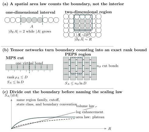
Three complementary meanings of boundary counting. A connected one-dimensional interval has a fixed number of cut links, whereas a two-dimensional region has boundary size proportional to its linear scale. An MPS or PEPS supplies exact Schmidt-rank bounds by counting virtual bonds severed by the same partition. Finally, the ratio $S_A/|\partial A|$ distinguishes an area-law plateau from logarithmic enhancement or volume-law growth only when the region family, cutoff, state class, and boundary convention are controlled.

Matrix product states

Across one bond, an MPS of bond dimension $D$ has Schmidt rank at most $D$:

$$\operatorname{rank}\rho_A \le D.$$

Entropy is maximized by a uniform spectrum on its support, so

$$S_A \le \ln D.$$

For a finite interval represented by an open-boundary MPS, two virtual bonds may be cut. Then

$$\operatorname{rank}\rho_A \le D_LD_R$$

and

$$S_A \le \ln D_L+\ln D_R.$$

For uniform bond dimension,

$$S_A\le2\ln D.$$

These are exact representational bounds. They do not assume that the MPS is a ground state.

Projected entangled-pair states

For a PEPS with virtual bond dimension $D$, suppose a region boundary cuts $n_\partial$ virtual legs. Before local projections, the Schmidt rank across the cut is at most

$$D^{n_\partial}.$$

Local maps cannot increase that rank, so

$$\operatorname{rank}\rho_A \le D^{n_\partial}$$

and

$$S_A \le n_\partial\ln D.$$

On a regular lattice,

$$n_\partial = O \left( |\partial_E A| \right).$$

Finite-$D$ PEPS therefore obey an area law by construction.

The converse does not follow

The implications

$$\begin{gathered} \text{finite-bond MPS} \\ \Downarrow \\ \text{one-dimensional area law}, \\ \text{finite-bond PEPS} \\ \Downarrow \\ \text{higher-dimensional area law} \end{gathered}$$

are straightforward. Their converses are not automatic.

A bound on von Neumann entropy controls one average of the Schmidt probabilities:

$$S_A = -\sum_\alpha p_\alpha\ln p_\alpha.$$

It does not fully control the tail

$$\varepsilon_D := \sum_{\alpha>D} p_\alpha$$

that determines truncation quality. Carefully constructed state families can obey a strict von Neumann area law while requiring large MPS bond dimension for accurate approximation.

Actual one-dimensional gapped ground states possess additional locality and spectral structure beyond a scalar entropy bound. That stronger structure underlies rigorous MPS approximation results.

Representation versus contraction

Even when a higher-dimensional state has a compact PEPS representation, evaluating its norm or observables can be computationally difficult. An entropy bound addresses representational capacity. It does not by itself provide:

• a stable optimization algorithm;
• efficient tensor-network contraction;
• a favorable condition number;
• a certified bond dimension at a requested error;
• immunity from metastable variational minima.

Area-law intuition explains why tensor networks are plausible. Algorithmic guarantees require more.

Local Hamiltonians and the Spectral Gap

Assumption ledger

Consider a family of lattice Hamiltonians

$$H_L = \sum_X h_X$$

with:

• finite local Hilbert-space dimension $q$;
• bounded interaction strength;
• finite-range or sufficiently fast-decaying interactions;
• bounded lattice degree;
• a ground state selected under stated degeneracy conditions;
• a spectral gap $\Delta>0$ uniform as $L\to\infty$.

The uniformity matters. Every finite Hamiltonian has discrete levels, but a gap

$$\Delta_L \longrightarrow0$$

does not define a gapped thermodynamic phase.

Locality and exponential clustering

Lieb–Robinson bounds provide an effective light cone for short-range lattice dynamics. Combined with a uniform spectral gap, they imply exponential decay of connected ground-state correlations under standard assumptions:

$$\begin{aligned} & \left| \langle O_XO_Y\rangle - \langle O_X\rangle \langle O_Y\rangle \right| \\ &\qquad \le C e^{-r/\xi} \|O_X\| \|O_Y\|. \end{aligned}$$

Here

$$r = \operatorname{dist}(X,Y),$$

and the correlation length is controlled schematically by

$$\xi \sim \frac{v_{\mathrm{LR}}}{\Delta},$$

up to model-dependent constants and locality conventions.

This result supports the boundary-layer intuition: degrees of freedom deep inside $A$ should not remain independently entangled with degrees of freedom far outside. Turning that intuition into an entropy theorem is nontrivial because entropy depends on the entire reduced spectrum, not only a few correlators.

The Rigorous One-Dimensional Area Law

The theorem-level statement

For broad families of one-dimensional quantum spin chains with finite local dimension, local bounded interactions, and a uniform nonzero spectral gap above a suitable ground state, the entanglement entropy across every cut is bounded independently of chain length:

$$S_{\mathrm{cut}} \le C \left( q, \Delta, J, R_0 \right).$$

Here $J$ is an interaction scale and $R_0$ a range or locality parameter. The precise theorem determines the allowed interaction family, boundary conditions, degeneracy assumptions, and functional form of $C$.

The central content is

$$\sup_L \sup_{\mathrm{cuts}} S_{\mathrm{cut}} < \infty.$$

This is stronger than observing saturation in a finite numerical window.

What the theorem does not claim

The theorem does not say:

• the entropy is exactly zero;
• the optimal bound is small;
• every gapped state is a product state;
• every excited state obeys the same bound;
• the entropy uniquely identifies the phase;
• one measured correlation length fixes the entropy coefficient;
• the same unrestricted result is proved in every dimension.

Early rigorous bounds had very unfavorable dependence on the gap and local dimension. Subsequent work improved both the conceptual route and quantitative estimates. The existence of a size-independent bound is more robust than any particular nonoptimal constant.

Exponential decay implies an area law on a line

A complementary one-dimensional result starts from the state rather than a parent Hamiltonian. Under the theorem’s correlation definition, a pure state on a line with exponential decay of correlations satisfies an area law.

This implication is specifically powerful in one dimension. Quantum data-hiding constructions show why small values of familiar two-point correlators do not generally control entanglement in arbitrary geometries. One must not replace the theorem’s assumptions with “the correlators I plotted look short ranged.”

Degenerate ground spaces

Ground-state degeneracy requires a state-selection rule. A theorem may bound:

• a unique ground state;
• every state in a ground space under additional assumptions;
• a specially chosen minimally entangled basis;
• low-energy states below a specified threshold.

If the ground space dimension grows rapidly, arbitrary superpositions can carry entanglement unrelated to the local energetic structure. State and sector must be specified.

Why a Gap Helps but Is Not the Definition

The gap is sufficient in the one-dimensional theorem

For the standard one-dimensional setting,

$$\begin{gathered} \text{locality and a uniform gap} \\ + \\ \text{finite local dimension} \\ \Downarrow \\ \text{area law}. \end{gathered}$$

The logical arrow includes all assumptions. Writing only

$$\Delta>0 \Longrightarrow \text{area law}$$

hides locality, dimensionality, and state selection.

A gap is not necessary

Gapless states can obey an area law. Finite-bond PEPS provide explicit critical examples with power-law correlations and strict area-law entropy. Certain gapless bosonic or gauge systems also retain a leading area term with subleading corrections.

Therefore:

$$\text{area law} \centernot\Longrightarrow \text{spectral gap}.$$

Short correlations are not the same datum

The GHZ state has bounded cut entropy but long-range order. Data-hiding states can have weak accessible correlations and large entanglement. Area law, spectral gap, and exponential clustering are related under controlled hypotheses but are not interchangeable definitions.

Higher Dimensions: Evidence and Open Status

The expected physical picture

For a short-range gapped ground state with correlation length $\xi$, a boundary-layer estimate counts degrees of freedom within distance $O(\xi)$ of the interface:

$$N_{\mathrm{layer}} \sim \frac{ |\partial A| \xi }{ a^d }.$$

If each boundary cell contributes at most a bounded amount, then

$$S_A \sim \alpha \frac{|\partial A|} {a^{d-1}}.$$

This is useful intuition, not a general proof. Correlations among boundary cells, gauge constraints, topological structure, and data hiding complicate a direct cell-by-cell argument.

What is established

Area laws are established or directly realized in many important settings, including:

• finite-bond PEPS and related tensor-network states;
• broad classes of free gapped bosonic and fermionic systems;
• commuting-projector and stabilizer fixed points;
• states related to known fixed points by finite-depth or quasi-local transformations;
• selected frustration-free and otherwise structured Hamiltonians;
• continuum vacuum states with a fixed ultraviolet regulator, where the leading divergence is boundary local.

Each item has its own assumptions. None should be silently promoted to all interacting Hamiltonians.

What remains open

For spatial dimension

$$d\ge2,$$

a general proof that every ground state of every finite-dimensional, short-range, interacting, uniformly gapped local Hamiltonian obeys a von Neumann area law remains unavailable without additional structure.

This is an open theorem problem, not evidence that ordinary gapped phases generically violate area laws. Numerical results, effective field theory, tensor-network constructions, and all standard fixed points strongly support area behavior across broad physical classes.

Quasi-adiabatic continuity

Along a smooth path of local Hamiltonians that remains gapped, quasi-adiabatic continuation maps local observables to quasi-local observables. This supports stability of the entanglement-scaling class within a gapped phase.

The generator has tails rather than strictly finite range. Bounding their accumulated contribution requires care, particularly in higher dimensions and for sharp entropy quantities. Quasi-adiabatic continuity is a powerful structural tool, not a one-line substitute for the missing unrestricted theorem.

Theorem and Evidence Ledger

Statement	Setting	Status
finite-$D$ MPS has bounded cut entropy	any 1D MPS	exact rank bound
finite-$D$ PEPS has boundary-bounded entropy	any PEPS region	exact rank bound
local uniformly gapped spin chain obeys an area law	broad 1D finite-dimensional families	rigorous theorem
exponential decay of correlations implies area law	pure states on a line under theorem assumptions	rigorous theorem
every interacting gapped local ground state obeys an area law	unrestricted $d\ge2$ setting	open in general
area law implies efficient MPS or PEPS simulation	arbitrary state family	false without stronger assumptions
gapless state must violate area law	any dimension	false

The assumptions column is part of every row, even when colloquial summaries omit it.

Area-Law Corrections and Violations

The leading label does not specify the full entropy expansion. Two states can share the same area term and differ in universal logarithms, constants, oscillations, or corner contributions. Conversely, a logarithmic enhancement can violate a strict area law without becoming a volume law.

One-dimensional conformal critical points

At a one-dimensional critical point described by a conformal field theory with central charge $c$, the ground-state entropy of an interval of length $\ell$ in an infinite system is

$$S_A(\ell) = \frac{c}{3} \ln \left( \frac{\ell}{a} \right) + s_1,$$

where $a$ is a short-distance cutoff and $s_1$ is nonuniversal. Because the boundary of an interval has fixed size, the logarithm violates a strict one-dimensional area law.

For a periodic chain of circumference $L$,

$$S_A(\ell,L) = \frac{c}{3} \ln \left[ \frac{L}{\pi a} \sin \left( \frac{\pi\ell}{L} \right) \right] + s_1.$$

The chord-length form automatically satisfies complement symmetry,

$$S_A(\ell,L) = S_A(L-\ell,L).$$

For an interval attached to an open boundary, the leading coefficient is halved:

$$S_A^{\mathrm{open}}(\ell) = \frac{c}{6} \ln \left( \frac{2\ell}{a} \right) + \ln g + \frac{s_1}{2}.$$

Here $\ln g$ is the boundary entropy for the chosen conformal boundary condition. These formulas belong to the scaling regime

$$a\ll \ell\ll L$$

or to the corresponding finite-size chord regime. They are not expected to fit a handful of lattice spacings.

Extended Fermi surfaces

For free fermions in $d>1$ with a codimension-one Fermi surface $\Gamma$, a smooth real-space region $R\Omega$ generally has

$$S_{R\Omega} \sim R^{d-1} \ln R.$$

More precisely, the leading geometric coefficient is governed by a Widom-type integral,

$$\begin{aligned} S_{R\Omega} &= \frac{ R^{d-1}\ln R }{ 12(2\pi)^{d-1} } \\ &\quad\times \int_{\partial\Omega} dA_x \int_{\Gamma} dA_k\, \left| \boldsymbol n_x \mathbin{\cdot} \boldsymbol n_k \right| \\ &\quad + O \left( R^{d-1} \right), \end{aligned}$$

up to degeneracy and convention factors. The normals $\boldsymbol n_x$ and $\boldsymbol n_k$ encode the relative orientation of the spatial boundary and Fermi surface.

The logarithm reflects a continuum of effectively one-dimensional gapless patches. The result is larger than an ordinary area law but still parametrically smaller than a volume law:

$$R^{d-1} \ll R^{d-1}\ln R \ll R^d.$$

An isolated point node does not produce the same enhancement. The dimension and codimension of the gapless manifold matter.

Goldstone modes

Spontaneous breaking of a continuous symmetry in $d>1$ produces gapless Goldstone modes. For a smooth region, the leading term can remain an area term while the finite-size tower of states and Goldstone sector contribute a universal logarithm:

$$\begin{aligned} S_A &= \alpha \frac{|\partial A|} {a^{d-1}} \\ &\quad + \frac{N_G}{2} \ln \left( \frac{ \rho_s R^{d-1} }{ c } \right) \\ &\quad + \gamma_{\mathrm{ord}} + \cdots. \end{aligned}$$

Here $N_G$ is the number of Goldstone modes, $\rho_s$ is a stiffness, $c$ is a mode velocity, and $\gamma_{\mathrm{ord}}$ depends on geometry and the ordered phase. The logarithmic coefficient contains universal information even though the leading coefficient $\alpha$ does not.

This example is a useful warning:

$$\begin{gathered} \text{gapless} \\ \centernot\Longrightarrow \\ \text{leading area-law violation}. \end{gathered}$$

Corners, defects, and physical boundaries

A nonsmooth entangling surface can add terms absent for a smooth surface. In two spatial dimensions, a corner of opening angle $\theta$ can contribute

$$-a(\theta)\ln(R/a),$$

with a universal function $a(\theta)$ at many critical points. Defects and physical boundaries can change both logarithmic and constant terms.

Comparing a square with a disk without accounting for corners mixes geometry with phase information. Reliable scaling studies use a controlled family of shapes or explicitly model corner terms.

Topological constant terms

For a gapped topologically ordered phase in two dimensions, a simply connected smooth region often has

$$S_A = \alpha \frac{|\partial A|}{a} - \gamma + o(1),$$

where

$$\gamma = \ln\mathcal D$$

is the topological entanglement entropy and $\mathcal D$ is the total quantum dimension. The state still obeys an area law. Its nontrivial information is in the subleading constant and in how constants combine across carefully chosen regions.

The dedicated topological-entanglement page linked above owns extraction protocols, anyon sectors, and their assumptions. The point here is only that

$$\begin{gathered} \text{area law} \\ \centernot\Longrightarrow \\ \text{topologically trivial}. \end{gathered}$$

State Class, Energy Density, and Temperature

An area law must name the class of states under discussion. Ground states, low-energy states, finite-energy-density eigenstates, time-evolved states, and thermal density operators obey different scaling expectations.

Ground and low-energy states

The standard area-law question concerns ground states of local Hamiltonians. A fixed number of localized quasiparticles typically changes the entropy by at most a boundary or constant correction. A number of excitations proportional to volume can change the leading law.

For a low-energy window, one must state how the energy cutoff scales with system size. “Low energy” can mean:

• a fixed number of excitations above the ground state;
• energy $E-E_0=O(1)$;
• an energy density approaching the ground-state density;
• every state below an extensive threshold.

These are not equivalent theorem statements.

Generic excited eigenstates

In a nonintegrable thermalizing system, typical finite-energy-density eigenstates are expected to have subsystem entanglement

$$S_A = s(e)V_A + o(V_A)$$

when $A$ is smaller than its complement. The coefficient $s(e)$ matches the thermodynamic entropy density at the eigenstate energy density under the usual eigenstate-thermalization assumptions.

Thus the same local Hamiltonian can have

$$\begin{aligned} \text{ground state} &: S_A \sim |\partial A|, \\ \text{typical excited eigenstate} &: S_A \sim |A|. \end{aligned}$$

An area law is a property of a state family, not of the Hamiltonian name alone.

Localized and constrained exceptions

Highly excited eigenstates in a fully many-body localized regime can obey an area law. This reflects an extensive set of quasi-local conserved quantities and failure of ordinary thermalization. The statement is phase- and model-dependent; it is not a theorem that every disordered nonthermal system is localized or area-law entangled.

Quantum many-body scars and fragmented Hilbert spaces can also support atypical low-entanglement eigenstates inside spectra dominated by volume-law states. Such states are exceptions selected by structure, not evidence that the surrounding spectrum obeys an area law.

Thermal density operators

For a Gibbs state,

$$\rho_\beta = \frac{e^{-\beta H}}{Z},$$

the subsystem von Neumann entropy generally contains an extensive thermal contribution:

$$\mathcal S(\rho_A) = s_{\mathrm{th}}(\beta)V_A + O \left( |\partial A| \right).$$

This does not contradict ground-state area laws. The global state is mixed, and $\mathcal S(\rho_A)$ is not a pure-state entanglement measure.

Mutual information cancels independent bulk entropy:

$$I(A:B) = \mathcal S(\rho_A) + \mathcal S(\rho_B) - \mathcal S(\rho_{AB}).$$

For a finite-range Hamiltonian decomposed as

$$H = H_A + H_B + H_{\partial},$$

the Gibbs variational principle gives

$$\begin{aligned} I(A:B) &\le \beta \operatorname{Tr} \left[ H_{\partial} \left( \rho_A\otimes\rho_B - \rho_{AB} \right) \right] \\ &\le 2\beta \left\| H_{\partial} \right\|. \end{aligned}$$

For bounded finite-range interactions,

$$\left\| H_{\partial} \right\| = O \left( |\partial_E A| \right),$$

so thermal mutual information has an area-law upper bound. It measures total correlation, including classical correlation, and should not be relabeled entanglement entropy.

Unitary dynamics

Starting from a product or area-law state, local unitary time evolution can spread entanglement outward from the boundary. At fixed time, locality constrains the affected layer. At times that grow with subsystem size, a thermalizing quench can produce a volume law:

$$S_A(t\to\infty) \sim s_{\mathrm{eq}}V_A$$

for subsystems smaller than their complements.

The order of limits matters:

$$\lim_{R\to\infty} \lim_{t\to\infty} \frac{S_A(t)}{|A|}$$

need not describe the same operational regime as

$$\lim_{t\to\infty} \lim_{R\to\infty} \frac{S_A(t)}{|A|}.$$

At any fixed $t$, a sufficiently large region has an interior outside the entanglement-growth light cone. At late times proportional to $R$, that interior can become entangled with the exterior.

Continuum and Gauge-Theory Caveats

Ultraviolet divergence

In a continuum quantum field theory, the algebra of arbitrarily short-distance modes near a sharp boundary produces ultraviolet-divergent entropy. With cutoff $a$,

$$S_A = c_{d-1} \frac{ \operatorname{Area}(\partial A) }{ a^{d-1} } + c_{d-2} \frac{ \mathcal G_{d-2} }{ a^{d-2} } + \cdots,$$

where $\mathcal G_{d-2}$ denotes an allowed geometric invariant. The leading coefficient depends on regulator and microscopic convention.

An “area law” in the continuum therefore often describes the leading divergence, not a finite universal number. Universal information is extracted from:

• logarithmic coefficients;
• shape derivatives;
• mutual information between separated regions;
• relative entropy;
• regulator-independent combinations of several entropies.

Taking $a\to0$ before specifying such a combination can erase the quantity one intended to compare.

Factorization is not automatic

The lattice notation

$$\mathcal H = \mathcal H_A \otimes \mathcal H_{\bar A}$$

need not survive literally in continuum field theory. Local von Neumann algebras are generally not type-I factors, and a sharp spatial split does not provide an ordinary tensor-product density matrix without a regulator or split construction.

The regulated lattice entropy is still physically useful, but the regulator is part of the definition. Claims of universality must identify which terms remain invariant when the regulator changes.

Constraints and gauge systems

Gauge constraints couple degrees of freedom across a boundary. The physical Hilbert space may fail to factorize into independent inside and outside factors. Different choices can include:

• an extended Hilbert space with edge modes;
• an algebraic entropy for a chosen local operator algebra;
• electric- or magnetic-center conventions;
• superselection-sector decompositions.

These choices can shift boundary-local terms. A reported area coefficient is incomplete unless the algebra, edge-mode prescription, and regulator are stated.

Why Area Laws Motivate Compression

Schmidt-rank capacity

Across a bipartition, write

$$\lvert\Psi\rangle = \sum_{i=1}^{r} \sqrt{\lambda_i} \lvert i_A\rangle \lvert i_B\rangle.$$

An exact representation with Schmidt-rank capacity $D$ requires

$$r\le D.$$

Because

$$S_A \le \ln r,$$

one obtains the necessary capacity condition

$$D \ge e^{S_A}.$$

For a one-dimensional area-law state with

$$S_A=O(1),$$

this lower-bound diagnostic does not force $D$ to grow exponentially with system size. For a volume-law state,

$$S_A \sim s\ell,$$

it requires

$$D \gtrsim e^{s\ell}$$

across a central cut.

This is the basic compression motivation.

Approximation is controlled by the tail

Keeping the $D$ largest Schmidt weights gives the normalized truncated state

$$\lvert\Psi_D\rangle = \frac{1}{ \sqrt{1-\epsilon_D} } \sum_{i=1}^{D} \sqrt{\lambda_i} \lvert i_A\rangle \lvert i_B\rangle,$$

where

$$\epsilon_D = \sum_{i>D} \lambda_i$$

is the discarded weight. Its fidelity with the exact state is

$$\left| \langle\Psi_D\vert\Psi\rangle \right|^2 = 1-\epsilon_D.$$

The entropy

$$-\sum_i\lambda_i\ln\lambda_i$$

does not determine $\epsilon_D$ at a chosen $D$. A very long tail of individually small weights can have modest von Neumann entropy yet demand large bond dimension for high-fidelity approximation.

Therefore

$$\begin{gathered} \text{small }S_A \\ \centernot\Longrightarrow \\ \text{small }\epsilon_D \\ \text{at every useful }D. \end{gathered}$$

Bounds on Rényi entropies with index below one, direct tail estimates, or theorem-specific structure can provide stronger approximation control.

Why one-dimensional gapped ground states are better behaved

The one-dimensional area-law theorem is part of a larger structural picture. Under appropriate assumptions, gapped ground states admit accurate matrix-product approximations with bond dimensions controlled by the gap, local dimension, interaction range, system size, and desired error.

The logical route is not merely

$$S_A=O(1) \Longrightarrow \text{efficient MPS}.$$

It uses locality and spectral information to control approximation across many cuts simultaneously. That extra structure is what turns an entropy statement into an algorithmically useful one.

Higher-dimensional contraction remains separate

For a PEPS with bond dimension $D$,

$$S_A \le n_{\partial}\ln D$$

is immediate. Evaluating norms or observables can nevertheless be computationally difficult because the two-dimensional virtual network must be contracted.

There are three separate questions:

1. Does a compact representation exist?
2. Can it be found from the Hamiltonian?
3. Can its observables be contracted accurately and efficiently?

An area law addresses the first question only indirectly. It does not answer the other two.

Numerical Diagnosis

Freeze the entropy ledger

Before fitting, record:

Item	Required choice
state	ground state, eigenstate, quench state, or mixed ensemble
entropy	von Neumann or specified Rényi index
region	interval, cylinder segment, square, disk, or another fixed family
boundary	lattice cut links or continuum geometric measure
system size	open, periodic, cylinder, torus, or infinite method
cutoff	lattice spacing, basis truncation, or field-theory regulator
extrapolation	subsystem size, total size, bond dimension, and numerical tolerance

Changing any row while keeping one fit formula can produce a false scaling claim.

One-dimensional workflow

For a gapped chain, test saturation with a finite-size-aware ansatz such as

$$\begin{aligned} S_A(\ell,L) &= S_\infty + A e^{-\ell/\xi_E} \\ &\quad + B e^{-(L-\ell)/\xi_E} + \cdots. \end{aligned}$$

For a periodic critical chain, compare with the chord length

$$x(\ell,L) = \frac{L}{\pi} \sin \left( \frac{\pi\ell}{L} \right)$$

and fit

$$S_A = \frac{c_{\mathrm{fit}}}{3} \ln \left( \frac{x}{a} \right) + s_1 + \cdots.$$

A trustworthy diagnosis should:

• exclude intervals comparable to the cutoff;
• enforce or verify $S_A(\ell)=S_A(L-\ell)$ for a pure state;
• repeat the fit over several total sizes;
• compare saturation and logarithmic candidates over the same window;
• vary the bond dimension and truncation tolerance.

Higher-dimensional workflow

Choose a family with controlled shape, for example rectangular regions of fixed aspect ratio. Record both

$$V_A(R)$$

and

$$B_A(R) = |\partial_E A|.$$

Then inspect

$$\frac{S_A(R)}{B_A(R)}.$$

Expected leading behavior is:

$$\begin{array}{c|c} \text{law} & S_A/B_A \\ \hline \text{area} & \text{constant} \\ \text{area}\times\ln R & \ln R \\ \text{volume} & R \end{array}$$

for regular $d$-dimensional regions. Subleading constants and corner logarithms can still curve finite-size data.

On cylinders, varying the circumference changes both the boundary length and the finite-size spectrum. Use several circumferences before identifying a two-dimensional asymptotic law.

Bond-dimension convergence

Every tensor-network estimate should be repeated at increasing bond dimension. A finite-$D$ MPS has

$$S_A\le\ln D$$

across a single cut, so it must eventually saturate even when the exact critical state has

$$S_A \sim \frac{c}{6}\ln\xi$$

for a half-infinite geometry.

Artificial saturation is detected by checking whether the apparent plateau moves with $D$. One should monitor:

• discarded weight;
• variational energy and energy variance;
• correlation length extracted from the transfer matrix;
• entropy and Rényi entropies;
• local observables and long-distance correlators.

Convergence of the energy alone does not prove convergence of the entanglement tail.

Model comparison and uncertainty

Area, logarithmically enhanced area, and volume fits can all look acceptable over a narrow size range. Use:

• the same data window for competing models;
• residual plots rather than only a fit coefficient;
• parameter stability under removal of the smallest sizes;
• physically constrained coefficients;
• uncertainty from finite size and bond dimension;
• independent gap and correlation-length diagnostics.

The strongest conclusion supported by limited data may be “consistent with an area law over accessible sizes,” not an asymptotic theorem.

Compact Worked Checks

Boundary doubling in one dimension

An open-chain prefix $A=\{1,\ldots,\ell\}$ has one cut link. An interval in the bulk has two. In a short-range entangled state with equal contribution $s_{\mathrm{cut}}$ per distant endpoint,

$$\begin{aligned} S_{\mathrm{prefix}} &\to s_{\mathrm{cut}}, \\ S_{\mathrm{bulk\ interval}} &\to 2s_{\mathrm{cut}}. \end{aligned}$$

The factor of two is geometry, not a change of phase.

Square-lattice Bell-pair state

Let every nearest-neighbor link carry an independent Bell pair, using separate local factors for different links. For an $m\times m$ square of sites,

$$|\partial_E A| = 4m.$$

Each severed pair contributes $\ln2$, so

$$S_A = 4m\ln2.$$

The region contains $m^2$ sites, but its entropy grows only linearly in $m$.

MPS capacity for a critical interval

Suppose the target entropy is

$$S_A(\ell) \simeq \frac{c}{3}\ln\ell.$$

An MPS interval has two virtual cuts and therefore

$$S_A\le2\ln D.$$

Entropy capacity alone requires

$$D \gtrsim \ell^{c/6}.$$

This polynomial lower bound is necessary, not sufficient: the Schmidt tail and simultaneous approximation of all cuts still matter.

Common Mistakes

• Calling every bounded entropy an area law. The family of spatial regions and its boundary measure must be specified.
• Using volume and boundary interchangeably in one dimension. An interval has length $O(\ell)$ but only one or two boundary cuts.
• Dropping theorem assumptions. The one-dimensional result uses locality, finite local dimension, a uniform gap, and a specified ground-state setting.
• Claiming a general higher-dimensional theorem. Broad evidence and many special results do not constitute an unrestricted proof.
• Treating a gap as the definition. Gapless area-law states and gapped states with nontrivial subleading structure both exist.
• Equating area law with product state. GHZ, symmetry-protected, symmetry-broken, and topologically ordered states can all obey area laws.
• Inferring efficient simulation from $S_A$ alone. Approximation tails, optimization, and contraction complexity remain.
• Fitting critical data with a finite-$D$ plateau. A matrix-product ansatz imposes an entropy ceiling.
• Ignoring corners or aspect ratio. Geometry can generate logarithms and constants.
• Calling thermal subsystem entropy entanglement. A mixed state’s von Neumann entropy includes thermal mixedness.
• Comparing bare continuum coefficients across regulators. The leading ultraviolet area coefficient is generally nonuniversal.
• Forgetting gauge-algebra choices. Edge modes and centers alter boundary-local terms.
• Using one system size. Area, logarithmic, and volume fits can mimic one another over short ranges.
• Using energy convergence as the only numerical check. Entanglement spectra and long-distance correlations can converge more slowly.

Exercises

1. Counting severed Bell pairs

On an infinite square lattice, associate an independent qubit with each end of every nearest-neighbor edge, and place the two qubits on each edge in a Bell state. Let $A$ be an $m\times n$ rectangular set of vertices.

1. Count the edges crossing from $A$ to its complement.
2. Compute $S_A$.
3. Compare the result with the number of vertices in $A$.
4. State which assumptions make the additivity exact.

Solution

The top and bottom sides each sever $m$ vertical edges. The left and right sides each sever $n$ horizontal edges. Therefore

$$|\partial_E A| = 2m+2n.$$

Every crossing edge carries one Bell pair. Tracing out its exterior qubit leaves

$$\rho_{\mathrm{edge}} = \frac{I_2}{2}$$

on the interior qubit, with entropy

$$\mathcal S(\rho_{\mathrm{edge}}) = \ln2.$$

The global state is a tensor product over edges, so the reduced state factorizes over severed pairs and pure interior pairs. Entropy is additive:

$$S_A = \left( 2m+2n \right) \ln2.$$

The volume is

$$|A| = mn.$$

At fixed aspect ratio and large $m,n$,

$$S_A = O(m+n), \qquad |A| = O(mn).$$

Exact additivity relies on independent tensor factors for different edges and on the state being an exact product of Bell pairs. In an interacting ground state, boundary contributions need not separate edge by edge even when the leading scaling remains an area law.

2. Endpoint dependence in a dimerized chain

Consider an infinite spin-$1/2$ chain in a product of nearest-neighbor singlets on bonds

$$(2j,2j+1).$$

For the interval

$$A = \{a,a+1,\ldots,b\},$$

determine the possible values of $S_A$ as the endpoint parities vary. Explain why microscopic oscillation does not violate the area law.

Solution

Only singlets cut by the two interval boundaries contribute. The left boundary cuts a singlet exactly when $a$ is odd, because site $a-1$ is then even and paired with $a$. The right boundary cuts a singlet exactly when $b$ is even, because $b$ is paired with $b+1$.

Thus the number of severed singlets is

$$n_{\mathrm{cut}} = \boldsymbol 1_{a\ \mathrm{odd}} + \boldsymbol 1_{b\ \mathrm{even}},$$

and

$$S_A = n_{\mathrm{cut}}\ln2.$$

The possible values are

$$S_A \in \left\{ 0,\ln2,2\ln2 \right\}.$$

They remain bounded independently of the interval length. The endpoint parity changes a microscopic boundary constant, not the scaling with the interior volume. Coarse-graining over a unit cell or fixing one endpoint convention removes the oscillation.

3. Rank bound for an MPS interval

An open-boundary MPS has bond dimensions no larger than $D$. Let $A$ be a connected interval strictly inside the chain.

1. Bound the Schmidt rank across $A\vert\bar A$.
2. Bound every Rényi entropy $S_\alpha(A)$ for $\alpha>0$.
3. Repeat for a prefix interval touching the left boundary.
4. Explain why neither bound proves accurate approximation of an arbitrary area-law state.

Solution

Cutting out a bulk interval severs two virtual bonds. The boundary virtual indices form a space of dimension at most

$$D\times D = D^2.$$

Therefore

$$\operatorname{rank}\rho_A \le D^2.$$

Any probability distribution supported on at most $D^2$ values has Rényi entropy no greater than the logarithm of its support:

$$S_\alpha(A) \le \ln D^2 = 2\ln D.$$

A prefix interval severs only one virtual bond, so

$$\operatorname{rank}\rho_A \le D, \qquad S_\alpha(A) \le \ln D.$$

These are capacity bounds for states already represented as MPS. An arbitrary state with bounded von Neumann entropy can have a slowly decaying Schmidt tail. The entropy bound does not guarantee that truncating to dimension $D$ gives small error, nor that one MPS approximates all cuts simultaneously.

4. Finite-depth circuit bound

Start from a product state of $q$-dimensional sites on a chain. Apply a depth-$t$ circuit of nearest-neighbor two-site unitaries, with disjoint gates in each layer. Let $A$ be a bulk interval.

1. Show that gates wholly inside $A$ or $\bar A$ do not change $S_A$.
2. Bound the number of gates that can cross the two boundaries.
3. Use operator Schmidt rank to prove a simple entropy bound.
4. Interpret the result as an area law.

Solution

A gate supported entirely inside $A$ acts as

$$U_A\otimes I_{\bar A},$$

and a gate entirely outside acts as

$$I_A\otimes U_{\bar A}.$$

Local unitaries do not change the Schmidt coefficients, so neither changes $S_A$.

At most one nearest-neighbor gate per layer crosses each endpoint. A bulk interval has two endpoints, so at most

$$2t$$

gates can cross its boundary.

A two-site unitary with one $q$-dimensional site on each side has operator Schmidt rank at most $q^2$. Acting with it can multiply the state Schmidt rank by at most $q^2$. Starting from rank one,

$$r_A \le \left( q^2 \right)^{2t} = q^{4t}.$$

Hence

$$S_A \le \ln r_A \le 4t\ln q.$$

The coefficient is a deliberately simple upper bound rather than an optimal one. Its important feature is independence from the interval length. At fixed circuit depth and local dimension, entanglement is controlled by the two boundary points.

5. Distinguishing three scaling laws

For hypercubic regions of linear size $R$ in $d>1$, suppose the candidate leading behaviors are

$$\begin{aligned} S_{\mathrm{area}}(R) &= \alpha R^{d-1}, \\ S_{\mathrm{Fermi}}(R) &= \kappa R^{d-1}\ln(R/a), \\ S_{\mathrm{volume}}(R) &= sR^d. \end{aligned}$$

1. Divide each by the boundary scale $R^{d-1}$.
2. Divide each by the volume scale $R^d$.
3. Give one diagnostic that distinguishes the logarithmic enhancement from a small volume coefficient.

Solution

Dividing by boundary scale gives

$$\begin{aligned} \frac{S_{\mathrm{area}}}{R^{d-1}} &= \alpha, \\ \frac{S_{\mathrm{Fermi}}}{R^{d-1}} &= \kappa\ln(R/a), \\ \frac{S_{\mathrm{volume}}}{R^{d-1}} &= sR. \end{aligned}$$

Thus the three cases are a plateau, logarithmic growth, and linear growth.

Dividing by volume gives

$$\begin{aligned} \frac{S_{\mathrm{area}}}{R^d} &= \frac{\alpha}{R}, \\ \frac{S_{\mathrm{Fermi}}}{R^d} &= \kappa \frac{\ln(R/a)}{R}, \\ \frac{S_{\mathrm{volume}}}{R^d} &= s. \end{aligned}$$

Both boundary-dominated cases vanish as $R\to\infty$, but at different rates.

One useful diagnostic is the logarithmic derivative of the boundary-normalized entropy:

$$g(R) = \frac{d}{ d\ln R } \left( \frac{S_A}{R^{d-1}} \right).$$

For the three idealized laws,

$$\begin{aligned} g_{\mathrm{area}} &= 0, \\ g_{\mathrm{Fermi}} &= \kappa, \\ g_{\mathrm{volume}} &= sR. \end{aligned}$$

In numerical work, the derivative must be estimated over several sizes and checked against subleading corner and finite-size terms.

6. Artificial saturation at finite bond dimension

A periodic critical chain has interval entropy

$$S_A(\ell) \simeq \frac{c}{3}\ln\ell+s_1$$

over the scaling window. A finite-$D$ MPS has

$$S_A\le2\ln D$$

for a bulk interval.

1. Find the length scale at which entropy capacity alone forces saturation.
2. Explain why the result is only an upper estimate of the useful correlation length.
3. Give three quantities to vary or monitor before concluding that the exact state is gapped.

Solution

Equating the leading critical entropy to the MPS ceiling gives

$$\frac{c}{3}\ln\ell_D+s_1 \simeq 2\ln D.$$

Therefore

$$\ell_D \simeq \exp \left[ \frac{3}{c} \left( 2\ln D-s_1 \right) \right]$$

or, ignoring the nonuniversal constant,

$$\ell_D \sim D^{6/c}.$$

This uses only entropy capacity. A particular variational MPS may develop a shorter transfer-matrix correlation length, and the actual Schmidt tail may require larger $D$ well before the ceiling is reached. The estimate is therefore not a prediction of the exact finite-entanglement exponent.

Before diagnosing a physical gap, increase $D$ and monitor at least:

• the location and height of the entropy plateau;
• the transfer-matrix correlation length;
• discarded weight or Schmidt-spectrum convergence;
• long-distance correlators;
• energy variance.

If the plateau and correlation length move systematically with $D$, the saturation is variational rather than physical.

7. Thermal mutual-information bound

Let

$$H = H_A+H_B+H_{\partial}$$

and let $\rho_{AB}=e^{-\beta H}/Z$. Define

$$\sigma_{AB} = \rho_A\otimes\rho_B.$$

1. Show that

$$\mathcal S(\sigma_{AB}) - \mathcal S(\rho_{AB}) = I(A:B)_\rho.$$

2. Use Gibbs free-energy minimality to derive

$$I(A:B)_\rho \le \beta \operatorname{Tr} \left[ H_{\partial} \left( \sigma_{AB}-\rho_{AB} \right) \right].$$

3. Obtain a norm bound and explain its scaling for finite-range interactions.
4. Explain why this is not an entanglement-area-law theorem.

Solution

Entropy is additive on a product state:

$$\mathcal S(\sigma_{AB}) = \mathcal S(\rho_A) + \mathcal S(\rho_B).$$

Therefore

$$\mathcal S(\sigma_{AB}) - \mathcal S(\rho_{AB}) = I(A:B)_\rho.$$

The Gibbs state minimizes

$$F_\beta(\omega) = \operatorname{Tr}(H\omega) - \beta^{-1}\mathcal S(\omega).$$

Thus

$$F_\beta(\rho_{AB}) \le F_\beta(\sigma_{AB}).$$

Rearranging gives

$$I(A:B)_\rho \le \beta \operatorname{Tr} \left[ H \left( \sigma_{AB}-\rho_{AB} \right) \right].$$

The two states have identical marginals, so

$$\operatorname{Tr} \left[ (H_A+H_B) \left( \sigma_{AB}-\rho_{AB} \right) \right] = 0.$$

Only the crossing interaction remains:

$$I(A:B)_\rho \le \beta \operatorname{Tr} \left[ H_{\partial} \left( \sigma_{AB}-\rho_{AB} \right) \right].$$

Using

$$\left\| \sigma_{AB}-\rho_{AB} \right\|_1 \le 2$$

and Hölder’s inequality,

$$I(A:B)_\rho \le 2\beta \left\| H_{\partial} \right\|.$$

For bounded finite-range interactions, $H_{\partial}$ contains only terms crossing the interface, so its norm is at most a constant times $|\partial_E A|$.

Mutual information counts all correlations in a mixed state. The bound does not isolate quantum entanglement, and $\mathcal S(\rho_A)$ itself still has a thermal volume term.

8. Audit an overbroad theorem claim

Assess the statement:

Every gapped quantum Hamiltonian has area-law ground states and is efficiently simulable by tensor networks.

Identify at least six missing assumptions or invalid implications, then write a defensible one-dimensional replacement.

Solution

The statement is overbroad for several independent reasons:

1. “Hamiltonian” does not specify short-range locality.
2. It does not require finite on-site Hilbert-space dimension or controlled bosonic truncation.
3. “Gapped” does not state a uniform thermodynamic gap.
4. It does not specify one spatial dimension, where the broad theorem is available.
5. Degenerate ground spaces and the selected state are unspecified.
6. A general unrestricted interacting theorem is not known in $d\ge2$.
7. Area-law entropy alone does not control the Schmidt tail.
8. Existence of a tensor-network representation does not imply it can be found efficiently.
9. PEPS contraction can remain computationally hard.
10. Numerical efficiency requires an error norm, observable class, and scaling target.

A defensible replacement is:

For broad one-dimensional finite-range quantum spin chains with fixed finite local dimension and a nonzero spectral gap uniform in system size, appropriately specified ground states obey a von Neumann entanglement area law. Under related locality and gap assumptions, they admit controlled matrix-product approximations, with resources depending on the gap, local data, system size, and target accuracy.

This version separates the theorem-level entropy statement from the additional approximation and algorithmic qualifications.

Summary

An area law is a scaling statement about a family of spatial regions:

$$S_A = O \left( |\partial A| \right)$$

or, in asymptotic language,

$$S_A = \alpha|\partial A| + \text{subleading terms}.$$

The boundary convention, state class, entropy, cutoff, geometry, and order of limits are part of the statement.

Exact boundary counting explains the law for Bell-pair states, finite-depth circuits, MPS, and PEPS. For broad one-dimensional local finite-dimensional systems, a uniform spectral gap yields a rigorous ground-state area law. In higher dimensions, area behavior is established in many major classes and strongly supported across ordinary gapped phases, but the unrestricted interacting theorem remains open.

Area laws motivate compression because they avoid the entropic necessity of exponentially large Schmidt rank. They do not by themselves control the Schmidt tail, produce an efficient optimization algorithm, or make higher-dimensional contraction easy.

The leading term is not the whole physics. Critical conformal systems, Fermi surfaces, Goldstone modes, corners, topological order, thermal mixed states, localized eigenstates, and continuum regulators all modify either the law or its interpretation. A reliable claim survives changes of region size, total size, bond dimension, and fit window, and it names every assumption that makes the comparison meaningful.

References

1. L. Bombelli, R. K. Koul, J. Lee, and R. D. Sorkin, “Quantum Source of Entropy for Black Holes”, Physical Review D 34, 373–383 (1986).
2. M. Srednicki, “Entropy and Area”, Physical Review Letters 71, 666–669 (1993).
3. G. Vidal, J. I. Latorre, E. Rico, and A. Kitaev, “Entanglement in Quantum Critical Phenomena”, Physical Review Letters 90, 227902 (2003).
4. P. Calabrese and J. Cardy, “Entanglement Entropy and Quantum Field Theory”, Journal of Statistical Mechanics P06002 (2004).
5. M. B. Hastings and X.-G. Wen, “Quasi-Adiabatic Continuation of Quantum States: The Stability of Topological Ground-State Degeneracy and Emergent Gauge Invariance”, Physical Review B 72, 045141 (2005).
6. M. B. Hastings and T. Koma, “Spectral Gap and Exponential Decay of Correlations”, Communications in Mathematical Physics 265, 781–804 (2006).
7. F. Verstraete and J. I. Cirac, “Matrix Product States Represent Ground States Faithfully”, Physical Review B 73, 094423 (2006).
8. F. Verstraete, M. M. Wolf, D. Pérez-García, and J. I. Cirac, “Criticality, the Area Law, and the Computational Power of Projected Entangled Pair States”, Physical Review Letters 96, 220601 (2006).
9. D. Gioev and I. Klich, “Entanglement Entropy of Fermions in Any Dimension and the Widom Conjecture”, Physical Review Letters 96, 100503 (2006).
10. A. Kitaev and J. Preskill, “Topological Entanglement Entropy”, Physical Review Letters 96, 110404 (2006).
11. M. Levin and X.-G. Wen, “Detecting Topological Order in a Ground State Wave Function”, Physical Review Letters 96, 110405 (2006).
12. M. B. Hastings, “An Area Law for One-Dimensional Quantum Systems”, Journal of Statistical Mechanics P08024 (2007).
13. N. Schuch, M. M. Wolf, F. Verstraete, and J. I. Cirac, “Entropy Scaling and Simulability by Matrix Product States”, Physical Review Letters 100, 030504 (2008).
14. M. M. Wolf, F. Verstraete, M. B. Hastings, and J. I. Cirac, “Area Laws in Quantum Systems: Mutual Information and Correlations”, Physical Review Letters 100, 070502 (2008).
15. J. Eisert, M. Cramer, and M. B. Plenio, “Area Laws for the Entanglement Entropy”, Reviews of Modern Physics 82, 277–306 (2010).
16. B. Bauer and C. Nayak, “Area Laws in a Many-Body Localized State and Its Implications for Topological Order”, Journal of Statistical Mechanics P09005 (2013).
17. F. G. S. L. Brandão and M. Horodecki, “An Area Law for Entanglement from Exponential Decay of Correlations”, Nature Physics 9, 721–726 (2013).
18. M. A. Metlitski and T. Grover, “Entanglement Entropy of Systems with Spontaneously Broken Continuous Symmetry”, Physical Review B 88, 115125 (2013).
19. H. Leschke, A. V. Sobolev, and W. Spitzer, “Scaling of Rényi Entanglement Entropies of the Free Fermi-Gas Ground State: A Rigorous Proof”, Physical Review Letters 112, 160403 (2014).
20. F. G. S. L. Brandão and M. Horodecki, “Exponential Decay of Correlations Implies Area Law”, Communications in Mathematical Physics 333, 761–798 (2015).
21. I. Arad, Z. Landau, U. Vazirani, and T. Vidick, “Rigorous RG Algorithms and Area Laws for Low Energy Eigenstates in 1D”, Communications in Mathematical Physics 356, 65–105 (2017).
22. J. I. Cirac, D. Pérez-García, N. Schuch, and F. Verstraete, “Matrix Product States and Projected Entangled Pair States: Concepts, Symmetries, Theorems”, Reviews of Modern Physics 93, 045003 (2021).

Cross-Links

• Entanglement Spectrum — rank, Schmidt tails, level structure, and symmetry data beyond entropy scaling.

• Mutual Information in Many-Body Systems — spatial and thermal boundary laws, separated-region decay, and correlator bounds.

• Volume Laws — extensive entropy in random, thermal, chaotic-eigenstate, and post-quench settings.

• Tensor Networks Preview — cut-capacity bounds, MPS, PEPS, MERA, and why an area law alone is not an algorithm.

• Matrix Product States Preview — one-dimensional Schmidt bonds, canonical gauges, transfer spectra, and finite-entanglement limitations.

• Entanglement and Criticality — the logarithmic critical exception, conformal central charge, and competing infrared cutoffs.

• Many-Body Entanglement Overview — partition, state class, measure, and scaling workflow.

• Entanglement Entropy in Many-Body Systems — entropy definition, spatial cuts, and the broad area/log/volume taxonomy.

• Thermal Entropy vs Entanglement Entropy — why mixed thermal subsystem entropy has a different interpretation.

• Variational Many-Body States — matrix-product and projected-pair variational ansätze.

• Connected Correlation Functions — clustering, correlation length, and connected observables.

• Boundary Conditions on Lattices — open, periodic, and twisted geometries.

• Thermodynamic Limit — scaling families, boundary corrections, and limit order.

• Quantum Phase Transitions — critical scaling, gaps, and finite-size analysis.

• Topological Order Preview — long-range entanglement and topological subleading terms.

• Luttinger Liquid Preview — one-dimensional gapless phases and conformal scaling.

• Schmidt Decomposition — Schmidt rank, weights, and truncation.

• Rényi Entropies — entropy-index dependence and spectrum sensitivity.

• Product States — the zero-entanglement reference class.

• Bell States — one entangled pair crossing a cut.

• Entanglement in Many-Body Physics — cross-volume orientation to phases, criticality, and simulation.