Tensor Networks Preview

A tensor network represents a high-rank many-body object by contracting a graph of lower-rank tensors. For a pure state in a local product basis,

$$\lvert\psi\rangle = \sum_{s_1,\ldots,s_N} \Psi_{s_1\cdots s_N} \lvert s_1\cdots s_N\rangle,$$

the coefficient array $\Psi_{s_1\cdots s_N}$ contains $q^N$ complex entries when every site has local dimension $q$. A tensor network replaces that generic array by a structured factorization. If $G=(V,E)$ is a graph with one physical index $s_v$ at each vertex and one virtual index $\alpha_e$ on each internal edge, then a broad class of tensor-network states has amplitudes

$$\Psi(\{s_v\}) = \sum_{\{\alpha_e\}} \prod_{v\in V} A_v^{s_v,\{\alpha_e:e\ni v\}}.$$

Each virtual index ranges over

$$\alpha_e = 1,\ldots,D_e,$$

where $D_e$ is the bond dimension of edge $e$. The network topology and bond dimensions determine which correlation and entanglement patterns are inexpensive to represent.

This is the central promise and the central limitation:

Tensor networks replace unrestricted many-body complexity by a chosen geometry of information flow.

They do not abolish exponential complexity. A network may require exponentially large bond dimensions, may be hard to contract even at modest bond dimension, or may be difficult to optimize. The useful question is therefore not merely whether a state has a tensor-network representation. Every finite state does, if sufficiently large tensors are allowed. The useful question is whether the state admits a controlled, contractible, and verifiably converged representation in the chosen network family.

Scope and Canonical Ownership

This page is the canonical conceptual preview of tensor networks as representations of many-body states. It owns:

• the graph, tensor, physical-index, and virtual-index dictionary;
• bond dimension and virtual gauge freedom;
• the general cut bound on Schmidt rank and entropy;
• the relationship between network geometry and entanglement structure;
• a comparison of matrix product states, tree tensor networks, projected entangled-pair states, and MERA;
• exact benchmark states and failure modes;
• the distinction between compact representation, efficient contraction, and successful optimization;
• physics-level guidance for selecting and validating a network family.

Nearby pages have narrower canonical roles:

• Variational Many-Body States compares MPS with determinant, Jastrow, paired, projected, and neural ansätze.
• Area Laws owns the rigorous and physical status of boundary-law scaling.
• Entanglement Spectrum owns Schmidt probabilities, truncation tails, and entanglement levels.
• Matrix Product States Preview owns canonical forms, transfer operators, injectivity, and one-dimensional details beyond this overview.
• Tensor Networks: Computational Guide owns method routing, convergence designs, and the error ledger for finite-bond calculations.
• Tensor-Network Simulation owns circuit-to-network translation, MPS gate execution, spacetime contraction trees, slicing, output-aware sampling, and simulator validation.
• DMRG Preview owns finite-system MPS optimization, local effective eigenproblems, sweeps, truncation, and convergence controls.
• Time-Dependent Variational Principle owns the general projection principle and its MPS application.
• The future Computational QM volume owns production contraction algorithms, tensor libraries, data structures, performance engineering, and benchmark implementations.

The boundary is representational rather than analytic versus numerical. This page explains what the network can express and what physical evidence makes that expression credible. It does not provide a software tutorial.

Convention Ledger

State and basis

Unless stated otherwise:

• $\lvert\psi\rangle$ is a normalized pure state;
• $N$ is the number of physical sites or local factors;
• $q_v=\dim\mathcal H_v$ is the local physical dimension;
• $q$ denotes a uniform local dimension;
• $s_v$ is a physical basis label;
• $\alpha_e$ is a contracted virtual label;
• $D_e$ is the virtual dimension on edge $e$;
• $\chi$ denotes a typical MPS bond dimension;
• logarithms are natural, so entropies are in nats.

The product basis is part of the representation. Reordering sites or changing orbitals can radically change the bond dimension needed for a given accuracy even though the physical state is unchanged.

Exact and approximate statements

An exact tensor network reproduces every coefficient $\Psi_{s_1\cdots s_N}$. An approximate network represents a state $\lvert\phi_D\rangle$ whose error is controlled under a declared metric, such as:

$$\left\lVert \lvert\psi\rangle - \lvert\phi_D\rangle \right\rVert,$$

the infidelity

$$1- \lvert\langle\psi\vert\phi_D\rangle\rvert^2,$$

or errors in selected observables. A small variational energy alone does not certify every one of these quantities.

State networks and operator networks

A state network has physical ket legs. An operator network has paired input and output legs. A density operator may be represented directly, through a purification, or through another positive parameterization. These choices have different positivity, normalization, and contraction properties.

Diagrams are contraction instructions

In a tensor diagram:

• a node denotes a multilinear array;
• a dangling leg denotes a free index;
• a joined pair of legs denotes a sum over their common index;
• cutting an internal leg exposes a virtual vector space;
• bending or crossing lines may carry convention-dependent meaning, especially for fermions.

A diagram is not automatically a quantum circuit. Generic tensors need not be unitary or isometric, and the drawing need not represent time evolution.

From One Tensor to a Network

A tensor as a multilinear map

A local tensor with one physical leg and $z$ virtual legs can be viewed as components

$$A^s_{\alpha_1\cdots\alpha_z}$$

or as a linear map

$$A: \bigotimes_{j=1}^{z} \mathbb C^{D_j} \longrightarrow \mathcal H_{\mathrm{phys}}.$$

This map viewpoint is especially useful for projected entangled-pair states: virtual entangled pairs live on graph edges, and local maps turn the incident virtual degrees of freedom into physical sites.

Contraction

Joining two tensor legs of equal dimension means summing over that index. For tensors $A_{i\alpha}$ and $B_{\alpha j}$,

$$C_{ij} = \sum_{\alpha=1}^{D} A_{i\alpha}B_{\alpha j}.$$

This is ordinary matrix multiplication when both tensors have rank two. Higher-rank networks generalize the same operation.

The final object depends on which legs remain open:

Open legs	Result
none	scalar, such as a norm or partition function
physical ket legs	state amplitudes
input and output legs	operator or channel
selected boundary legs	effective environment or boundary state

Parameter count is only a first diagnostic

For a regular network with $N$ site tensors, physical dimension $q$, coordination number $z$, and uniform bond dimension $D$, a site-dependent raw parameter count scales as

$$O \left( NqD^z \right).$$

This can be vastly smaller than $q^N$. But raw parameter count does not answer three decisive questions:

1. How large must $D$ become for the target state and error tolerance?
2. How difficult is it to contract the resulting network?
3. Can an optimization procedure find an accurate tensor set?

Gauge redundancy also means that different tensor entries can represent the same physical state, so the raw count overestimates the true number of state-space directions.

Virtual Gauge Freedom

Consider two neighboring tensors joined along an internal bond. In matrix notation, their contraction contains

$$AB.$$

For any invertible matrix $X$ on the shared virtual space,

$$AB = \left(AX\right) \left(X^{-1}B\right).$$

Thus the transformations

$$\begin{aligned} A&\longrightarrow AX, \\ B&\longrightarrow X^{-1}B \end{aligned}$$

leave the physical amplitudes unchanged.

Consequences

Virtual gauge freedom means:

• individual tensor entries are not observables;
• norms of neighboring tensors can be redistributed without changing the state;
• optimization can contain flat or poorly conditioned directions;
• canonical or isometric gauges can expose Schmidt data and improve stability;
• comparing tensors from two calculations requires gauge alignment or gauge-invariant quantities.

For an open MPS, sequential canonical gauges are particularly powerful because the graph is a chain. Networks with loops, such as PEPS, do not generally admit one global canonical form with all the same properties.

Gauge freedom is not physical gauge symmetry

Virtual basis redundancy and a physical gauge constraint are different ideas. The first is a nonuniqueness of tensor coordinates. The second restricts physical states and observables. Symmetric or gauge-invariant tensor networks can connect them structurally, but they should not be identified merely because both use the word “gauge.”

The General Cut Bound

The most direct link between tensor networks and entanglement comes from cutting virtual bonds.

Partition the physical vertices into $A$ and $\bar A$. Suppose removing an edge set

$$\partial_G A$$

disconnects all tensors carrying physical legs in $A$ from those carrying physical legs in $\bar A$. After exposing those cut indices, the state can be written as

$$\lvert\psi\rangle = \sum_{\boldsymbol\alpha} \lvert L_{\boldsymbol\alpha}\rangle_A \otimes \lvert R_{\boldsymbol\alpha}\rangle_{\bar A},$$

where the compound cut label has dimension

$$\dim\boldsymbol\alpha = \prod_{e\in\partial_G A} D_e.$$

The vectors on either side need not be orthogonal, so this is not necessarily a Schmidt decomposition. It is nevertheless a decomposition with at most that many product terms. Therefore

$$\operatorname{SchmidtRank}_{A\vert\bar A} \le \prod_{e\in\partial_G A} D_e.$$

Equivalently,

$$\operatorname{rank}\rho_A \le \prod_{e\in\partial_G A} D_e.$$

Because entropy cannot exceed the logarithm of the support dimension,

$$S_A \le \sum_{e\in\partial_G A} \ln D_e.$$

For uniform bond dimension $D$ and $n_{\partial}$ cut edges,

$$S_A \le n_{\partial}\ln D.$$

The same rank ceiling bounds every Rényi entropy with positive index:

$$S_\alpha(A) \le n_{\partial}\ln D, \qquad \alpha>0.$$

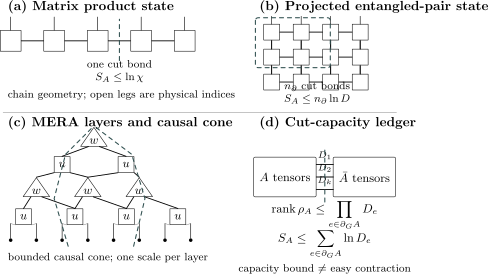
A representation ledger for common tensor-network geometries. An MPS cut severs one virtual bond, a PEPS region boundary severs a number of bonds proportional to its lattice perimeter, and a MERA organizes tensors by length scale with a bounded causal cone for local observables. In any network, a separating edge set gives $\operatorname{rank}\rho_A\le\prod_eD_e$ and $S_A\le\sum_e\ln D_e$. These are capacity bounds; they do not guarantee accurate approximation, efficient contraction, or successful optimization.

Min-cut language

Several different virtual cuts may separate the same physical partition. Taking the smallest cut capacity gives the strongest immediate graph bound:

$$S_A \le \min_{\mathcal C:A\vert\bar A} \sum_{e\in\mathcal C} \ln D_e.$$

This resembles a discrete minimal-surface rule, but it is generally an upper bound, not an equality. Special networks and limits can make geometric cut formulas much sharper. A generic tensor network does not establish a holographic entropy formula.

What the bound does not say

The cut bound does not imply that:

• every virtual channel is used;
• the reduced state has a flat spectrum;
• the entropy saturates the bound;
• a state with smaller entropy is accurately approximated at that bond dimension;
• the network can be contracted efficiently;
• the graph matches the locality of the Hamiltonian;
• the tensors found by an optimizer are close to the best tensors at that $D$.

The zero state satisfies every rank bound but is not a normalized physical state. A product state embedded in a large-$D$ network may use only one virtual channel. Capacity is not realized entanglement.

Schmidt Tails and Approximation Quality

For one bipartition, write the Schmidt decomposition

$$\lvert\psi\rangle = \sum_{a=1}^{R} \sqrt{p_a} \lvert a\rangle_A \lvert a\rangle_{\bar A},$$

with

$$p_1\ge p_2\ge\cdots\ge0, \qquad \sum_a p_a=1.$$

Keeping the first $\chi$ terms leaves discarded weight

$$\varepsilon_\chi := \sum_{a>\chi} p_a.$$

The unnormalized truncated state

$$\lvert\widetilde\psi_\chi\rangle = \sum_{a=1}^{\chi} \sqrt{p_a} \lvert a\rangle_A \lvert a\rangle_{\bar A}$$

satisfies

$$\left\lVert \lvert\psi\rangle - \lvert\widetilde\psi_\chi\rangle \right\rVert^2 = \varepsilon_\chi.$$

After normalization,

$$\lvert\psi_\chi\rangle = \frac{ \lvert\widetilde\psi_\chi\rangle }{ \sqrt{1-\varepsilon_\chi} },$$

the squared fidelity is

$$\lvert \langle\psi\vert\psi_\chi\rangle \rvert^2 = 1-\varepsilon_\chi.$$

This is why the entanglement spectrum, not entropy alone, controls local Schmidt truncation.

Two states can have the same entropy while having very different $\varepsilon_\chi$. An entropy area law therefore motivates low-rank approximation but does not, by itself, certify a bond dimension at a requested global error.

A Family Map

Network	Graph geometry	Natural setting	Cut capacity	Characteristic caution
MPS	one-dimensional chain	1D ground states and dynamics	one bond per chain cut	volume-law growth forces large $\chi$
tree tensor network	hierarchy without loops	clusters and hierarchical correlations	path-dependent, often logarithmic	lattice translations are not built in automatically
PEPS	lattice-matched graph	2D and higher-dimensional states	boundary-edge count	compact representation need not be easy to contract
MERA	layered isometries and disentanglers	scale-resolved and critical states	bounded cuts per scale	architecture and optimization are more involved

These are families, not individual algorithms. A network geometry specifies an ansatz class and contraction problem. DMRG, variational updates, imaginary-time evolution, and environment methods are procedures for selecting or evaluating tensors within such classes.

Matrix Product States

An open-boundary matrix product state on a chain of $L$ sites has coefficients

$$\Psi_{s_1\cdots s_L} = \ell^{\mathsf T} A_1^{s_1} A_2^{s_2} \cdots A_L^{s_L} r.$$

Equivalently, one may absorb the boundary vectors into the first and last tensors and write

$$\begin{aligned} \Psi_{s_1\cdots s_L} &= \sum_{\alpha_1,\ldots,\alpha_{L-1}} A_1^{s_1}{}_{\alpha_1} \\ &\quad {}\times A_2^{s_2}{}_{\alpha_1\alpha_2} \cdots A_L^{s_L}{}_{\alpha_{L-1}}. \end{aligned}$$

The tensor at site $i$ has dimensions

$$q_i \times \chi_{i-1} \times \chi_i, \qquad \chi_0=\chi_L=1.$$

The raw parameter count is therefore

$$\sum_{i=1}^{L} q_i\chi_{i-1}\chi_i.$$

For uniform $q$ and $\chi$, this is

$$O \left( Lq\chi^2 \right),$$

before gauge redundancy and symmetry reduction are taken into account.

Exact construction by sequential singular-value decomposition

Every finite-chain state admits an exact MPS. Reshape the coefficient tensor across the first cut:

$$\Psi_{s_1,(s_2\cdots s_L)}.$$

Its singular-value decomposition gives

$$\Psi_{s_1,(s_2\cdots s_L)} = \sum_{\alpha_1=1}^{\chi_1} U^{[1]}_{s_1\alpha_1} \sigma^{[1]}_{\alpha_1} V^{[1]*}_{(s_2\cdots s_L),\alpha_1}.$$

Treat

$$\sigma^{[1]}V^{[1]\dagger}$$

as a new tensor with indices $\alpha_1,s_2,\ldots,s_L$, reshape across the next cut, and repeat. The exact bond dimension at cut $i$ can be chosen as the Schmidt rank

$$\chi_i = \operatorname{SchmidtRank}_{1\cdots i\vert i+1\cdots L}.$$

For uniform local dimension,

$$\chi_i \le q^{\min(i,L-i)}.$$

A generic state nearly saturates this exponential ceiling near the middle of the chain. Thus exact MPS existence is not an efficiency result.

Entanglement capacity

A chain cut severs one MPS bond, so

$$S_{1\cdots i} \le \ln\chi_i.$$

A finite interval strictly inside an open chain severs two bonds. If its left and right bond dimensions are $\chi_L$ and $\chi_R$, then

$$S_A \le \ln\chi_L + \ln\chi_R.$$

Uniform finite-$\chi$ MPS therefore obey a one-dimensional area law by construction. The converse requires additional conditions; an arbitrary state with bounded von Neumann entropy need not have a rapidly decaying Schmidt tail at every cut.

Product states

At bond dimension one, every tensor is a local vector:

$$A_i^{s_i} = a_i^{s_i}.$$

The amplitude factorizes,

$$\Psi_{s_1\cdots s_L} = \prod_{i=1}^{L} a_i^{s_i},$$

so

$$\lvert\psi\rangle = \bigotimes_{i=1}^{L} \lvert a_i\rangle.$$

This is the exact $\chi=1$ benchmark. A code or derivation that cannot reproduce this limit has a contraction, indexing, or normalization error.

A bond-dimension-two GHZ state

The $L$-qubit state

$$\lvert\mathrm{GHZ}_L\rangle = \frac{ \lvert0\cdots0\rangle + \lvert1\cdots1\rangle }{\sqrt2}$$

has an exact translation-invariant bulk MPS with

$$A^0 = \begin{pmatrix} 1&0 \\ 0&0 \end{pmatrix}, \qquad A^1 = \begin{pmatrix} 0&0 \\ 0&1 \end{pmatrix},$$

and boundary vectors

$$\ell^{\mathsf T} = \frac1{\sqrt2} \begin{pmatrix} 1&1 \end{pmatrix}, \qquad r = \begin{pmatrix} 1 \\ 1 \end{pmatrix}.$$

If the physical string contains both $0$ and $1$, the product of diagonal projectors vanishes. The two uniform strings each have amplitude $1/\sqrt2$.

Every nontrivial bipartition has

$$S_A = \ln2,$$

yet the connected correlator satisfies

$$\langle Z_iZ_j\rangle_c = 1$$

for arbitrarily separated sites in the symmetric finite-volume state. Low bond dimension and bounded entropy do not imply short-range correlations.

Transfer operators and correlation length

For a translation-invariant MPS, define the transfer operator

$$\mathcal E = \sum_s A^s\otimes\overline{A^s}.$$

With an inserted local operator $O$,

$$\mathcal E_O = \sum_{s,s'} \langle s'\lvert O\rvert s\rangle A^s\otimes\overline{A^{s'}}.$$

After normalizing the largest transfer eigenvalue to one, a nondegenerate leading eigenvalue and subleading magnitude $\lvert\lambda_2\rvert<1$ produce the characteristic length

$$\xi_\chi = -\frac1{ \ln\lvert\lambda_2\rvert }.$$

Finite-$\chi$ MPS can therefore impose an artificial finite correlation length near criticality. Degenerate leading eigenvalues or non-injective structure, as in the GHZ example, require separate treatment and can support nondecaying correlations.

The dedicated MPS page develops canonical forms, injectivity, transfer spectra, and matrix-product operators in greater depth.

Tree Tensor Networks

A tree tensor network organizes physical sites through a loop-free hierarchy. In a binary tree, pairs of local spaces map into coarser effective spaces, then pairs of effective spaces are combined again.

If the coarse-graining tensors are isometries $w$, one convention is

$$w^dagger w = I_{mathrm{coarse}}.$$

The adjoint $w^dagger$ embeds a coarse state into the finer space, while $w$ removes directions excluded by the selected effective subspace.

Entanglement from tree cuts

For a contiguous block of length $\ell$ in a balanced one-dimensional binary tree, a separating cut can cross only a bounded number of bonds at each of

$$O(\ln\ell)$$

layers. With uniform bond dimension $D$,

$$S_A = O \left( \ln\ell\,\ln D \right).$$

The coefficient depends on the tree architecture and the alignment of the interval with the hierarchy. A different physical region can cut many more branches.

Strengths and limitations

Tree networks offer:

• exact contraction without loop environments;
• a natural hierarchy of length scales;
• efficient access to selected reduced states;
• flexible adaptation to clusters, orbitals, or irregular graphs.

They also impose a preferred hierarchy. Ordinary lattice translations and equivalent treatment of every cut are not automatic. A poor tree can place strongly entangled degrees of freedom far apart in the network and force large bond dimensions.

Projected Entangled-Pair States

Projected entangled-pair states generalize the virtual-bond construction to lattices and general graphs. Place a maximally entangled virtual pair on every edge:

$$\lvert\Phi_{D_e}\rangle_e = \frac1{\sqrt{D_e}} \sum_{\alpha=1}^{D_e} \lvert\alpha\rangle_{e,L} \lvert\alpha\rangle_{e,R}.$$

At each vertex $v$, apply a local map from all incident virtual spaces to the physical site:

$$P_v: \bigotimes_{e\ni v} \mathbb C^{D_e} \longrightarrow \mathcal H_v.$$

The PEPS is

$$\lvert\psi_{\mathrm{PEPS}}\rangle = \left( \bigotimes_{v\in V}P_v \right) \left( \bigotimes_{e\in E} \lvert\Phi_{D_e}\rangle_e \right).$$

Expanding the virtual pairs reproduces the graph-contraction formula from the opening section.

Boundary-law capacity

If a spatial region $A$ cuts $n_{\partial}$ virtual edges of uniform dimension $D$, then

$$\operatorname{rank}\rho_A \le D^{n_{\partial}}$$

and

$$S_A \le n_{\partial}\ln D.$$

For a regular region on a local $d$-dimensional lattice,

$$n_{\partial} = O \left( \lvert\partial A\rvert \right).$$

Finite-$D$ PEPS therefore satisfy an area-law upper bound by construction.

Square-lattice parameter count

A bulk square-lattice tensor has one physical and four virtual legs:

$$A^s_{\ell r u d}.$$

For site-dependent tensors with uniform dimensions, the raw count scales as

$$O \left( NqD^4 \right).$$

Translation invariance can reduce the number of distinct tensors, but it does not make their contraction trivial.

Compact representation is not easy contraction

The norm

$$\langle\psi_{\mathrm{PEPS}} \vert \psi_{\mathrm{PEPS}}\rangle$$

is a double-layer network. Each ket virtual leg pairs with a bra virtual leg, giving effective dimension

$$D^2.$$

Contracting one row of a two-dimensional network into the next generally grows an intermediate boundary object. Exact contraction cost can therefore increase exponentially with the lattice width even when $D$ is fixed.

Worst-case exact PEPS contraction is #P-complete under the standard complexity-theoretic formulation. This theorem does not say that every physically structured PEPS instance is equally hard. It does say that finite bond dimension and an area law do not furnish a universal efficient classical contraction algorithm.

Practical PEPS methods use approximate environments, boundary MPS, corner constructions, tensor renormalization, Monte Carlo, or problem-specific structure. Their implementation and error control belong to computational-method pages.

Correlations and phases

Finite-$D$ PEPS can describe much more than short-range trivial states. The family includes examples with:

• symmetry breaking;
• algebraic correlations;
• topological order;
• symmetry-protected structure;
• exact parent Hamiltonians;
• nontrivial boundary theories and entanglement spectra.

In particular, finite PEPS bond dimension does not force a finite physical correlation length. This contrasts with the generic injective finite-$\chi$ MPS transfer-matrix picture and is one reason one-dimensional intuition should not be imported uncritically into two dimensions.

Multiscale Entanglement Renormalization Ansatz

MERA augments a hierarchy of isometries with disentanglers that act across block boundaries before coarse-graining. In a common convention, a disentangler $u$ is unitary,

$$u^dagger u = uu^dagger = I,$$

while a coarse-graining tensor $w$ is isometric,

$$w^dagger w = I.$$

These identities allow tensors outside the causal cone of a local observable to cancel against their adjoints.

Bounded causal cones

To compute a local expectation value, follow the operator upward through the network. In a properly designed MERA, its support remains bounded in width as the number of layers grows. A system of linear size $L$ has

$$O(\ln L)$$

layers, so local observables can be evaluated without contracting the entire network at once.

The precise cost depends on the branching structure, dimension, bond dimension, and update scheme. “Bounded causal cone” is a structural statement, not a universal cost formula independent of architecture.

Entanglement by scale counting

For a one-dimensional interval of length $\ell$, a MERA cut can cross only a bounded number of bonds per layer over

$$O(\ln\ell)$$

relevant layers. Hence

$$S_A = O \left( \ln\ell\,\ln D \right).$$

This architecture is naturally compatible with the logarithmic interval entropy of many one-dimensional critical ground states. A scale-invariant MERA repeats tensors across layers and can encode algebraic correlations governed by scaling operators of an ascending map.

What MERA does not establish

A MERA fit does not by itself prove:

• exact conformal invariance;
• a unique continuum field theory;
• a holographic dual;
• that all critical exponents have converged;
• that finite-size and finite-bond effects are negligible.

The architecture organizes information by scale. Physical claims still require symmetry, correlation, spectrum, and convergence evidence.

Area Laws and Compression

The safest implication is from a network to an entanglement-capacity bound:

$$\begin{gathered} \text{bounded cut capacity} \\ \Longrightarrow \\ \text{bounded Schmidt rank and entropy}. \end{gathered}$$

The reverse implication is more delicate:

$$\begin{gathered} \text{small }S_A \\ \not\Longrightarrow \\ \text{small global network at certified error}. \end{gathered}$$

Why one-dimensional gapped systems are favorable

For broad classes of one-dimensional finite-range Hamiltonians with fixed local dimension and a spectral gap uniform in system size, ground states obey an entanglement area law. Stronger locality and spectral information then support controlled MPS approximation results.

The assumptions matter:

• one spatial dimension;
• finite local Hilbert-space dimension;
• local or sufficiently decaying interactions;
• a gap that does not close with system size;
• a specified ground-state and degeneracy setting;
• an explicit norm, observable, or energy accuracy target.

An isolated entropy bound is not the whole theorem package.

Critical chains

At a one-dimensional conformal critical point, an interval often has leading entropy

$$S_A \sim \kappa\ln\ell.$$

The MPS capacity bound requires

$$\ln\chi \gtrsim \kappa\ln\ell,$$

or

$$\chi \gtrsim \ell^\kappa$$

for exact capacity at that cut. Finite-$\chi$ MPS produce a finite-entanglement correlation length and can mimic a gapped state beyond it. Critical fits should therefore vary both system size and bond dimension.

MERA distributes entanglement over scales and can encode logarithmic growth at fixed local bond dimension, though its tensors and optimization remain nontrivial.

Volume-law states

If a chain bipartition has

$$S_A \sim s\ell,$$

then an exact MPS requires

$$\chi \ge e^{s\ell}.$$

This exponential demand appears in generic highly excited states and during sufficiently long real-time evolution after a global quench. It is an entanglement barrier for chain-ordered MPS, not a claim that every observable becomes immediately inaccessible by every method.

Network topology matters

Bond dimension cannot be compared without the graph. A bond of dimension $D$ in an MPS, a PEPS, and a MERA contributes to different cuts and contraction costs. A network with nonlocal edges can represent some volume-law partitions at modest local $D$ by allowing many edges to cross the physical cut, but the graph may then lose locality or become difficult to contract.

The meaningful comparison reports:

• network family and topology;
• physical-site ordering;
• every relevant bond dimension;
• parameter count after symmetry constraints when useful;
• contraction or environment approximation;
• measured error at matched computational resources.

Symmetry in Virtual Spaces

An exact global symmetry can be built into local tensors rather than recovered approximately after optimization. For an Abelian charge, tensor entries vanish unless the oriented charges satisfy a local selection rule of the form

$$q_s + \sum_{e\ni v} \eta_{ve}q_{\alpha_e} = Q_v,$$

where $\eta_{ve}=\pm1$ records the chosen orientation and $Q_v$ is the tensor’s net charge.

Block structure

Charge conservation decomposes virtual spaces into sectors:

$$\mathbb C^{D_e} = \bigoplus_q \left( \mathbb C^{m_{e,q}} \otimes \mathcal V_q \right).$$

Here $\mathcal V_q$ carries charge $q$ and $m_{e,q}$ is its degeneracy. Contractions become block sparse, forbidden sectors are absent, and the state remains in the intended global symmetry sector up to numerical precision.

Virtual symmetry carries physical information

Virtual symmetry is not only a speed device. In one-dimensional MPS, projective actions on virtual bonds help distinguish symmetry-protected phases. In PEPS, virtual symmetries can encode topological sectors and anyonic structure.

These statements require the relevant injectivity, symmetry, and phase assumptions. A visually symmetric tensor diagram is not by itself a phase classification.

Fermionic and Constrained Networks

Tensor diagrams for ordinary complex vector spaces allow line crossings to be rearranged without a sign. Fermionic Fock spaces require parity-aware conventions. Valid approaches include:

• Jordan–Wigner mappings with explicit strings;
• graded tensor products;
• fermionic swap gates;
• parity-symmetric local tensors;
• ordering conventions retained throughout every contraction.

Ignoring these choices can change signs and therefore the physical state.

Gauge theories and constrained Hilbert spaces similarly require invariant local tensors, projectors, or symmetry-adapted virtual spaces. The virtual coordinate gauge freedom discussed earlier does not enforce Gauss’s law automatically.

Operators and Mixed States

Tensor-network structure is useful beyond pure state vectors.

Matrix product operators

An operator on a chain can be represented as

$$O = \sum_{\substack{s_1,\ldots,s_L\\s'_1,\ldots,s'_L}} O_{s_1\cdots s_L}^{s'_1\cdots s'_L} \lvert s'_1\cdots s'_L\rangle \langle s_1\cdots s_L\rvert,$$

with coefficients factorized as

$$O_{s_1\cdots s_L}^{s'_1\cdots s'_L} = \ell^{\mathsf T} W_1^{s'_1s_1} W_2^{s'_2s_2} \cdots W_L^{s'_Ls_L} r.$$

This is a matrix product operator, or MPO. Local and finite-range Hamiltonians often admit MPO representations with bond dimensions that remain modest as $L$ grows, though the exact value depends on interaction range, symmetries, and compression choices.

Applying an MPO of bond dimension $D_W$ to an MPS of bond dimension $\chi$ can produce an intermediate state with bond dimension as large as

$$\chi' \le D_W\chi$$

on each corresponding bond before compression. Repeated application without truncation can therefore increase cost rapidly.

Density operators

A mixed state may be represented directly as an MPO,

$$\rho = \sum_{\mathbf s,\mathbf s'} \rho_{\mathbf s}^{\mathbf s'} \lvert\mathbf s'\rangle \langle\mathbf s\rvert.$$

Hermiticity and unit trace can be imposed or repaired, but positivity is more delicate. Truncating a generic operator-network expansion can create small negative eigenvalues even when the target density operator is positive.

A purification avoids this problem structurally. Introduce ancillas and represent

$$\lvert\Psi\rangle_{SA}$$

as a tensor-network state, then define

$$\rho_S = \operatorname{Tr}_A \lvert\Psi\rangle \langle\Psi\rvert.$$

Positivity is automatic, although the ancilla increases local dimensions and purification entanglement is not unique.

Thermal states

Starting from a purification of the infinite-temperature identity, imaginary-time evolution formally gives

$$\lvert\Psi(\beta)\rangle \propto \left( e^{-\beta H/2} \otimes I_A \right) \lvert\Psi(0)\rangle.$$

Tracing out the ancilla yields

$$\rho_\beta = \frac{e^{-\beta H}}{Z}.$$

In practice, imaginary-time discretization, operator approximation, truncation, and normalization all require convergence checks. Thermal tensor-network algorithms belong to computational-method pages; the representational point is that mixed-state complexity can be shifted into a purified state or operator bond dimension.

Operator entanglement

An operator can be treated as a vector in Hilbert–Schmidt space by grouping its input and output indices. Its Schmidt spectrum across a spatial cut controls MPO compression in much the same way that state Schmidt data control MPS compression.

Operator entanglement is not ordinary state entanglement unless the operator has been mapped to a normalized state under a declared convention. It becomes especially important in time evolution, quantum channels, and scrambling, where an initially local operator can spread and require rapidly growing MPO bond dimension. Operator Entanglement and Scrambling Preview owns that doubled-space construction and its diagnostic limits.

Contraction Geometry

The value of a tensor network is obtained only after a contraction order is chosen. Different orders can create intermediate tensors with very different ranks and sizes.

Chains

An open MPS norm can be contracted from left to right. If the MPS bond dimension is $\chi$, the boundary object remains a $\chi\times\chi$ matrix rather than acquiring one index for every physical site. Local expectation values and correlation functions are therefore polynomial in $L$ and $\chi$ under standard assumptions.

The exact exponent of $\chi$ depends on canonical gauge, observable structure, boundary conditions, and implementation. A quoted cost such as $O(L\chi^3)$ is meaningful only with those conventions stated.

Loops and width

In a PEPS, contracting part of the lattice leaves an effective tensor along the uncontracted boundary. Its dimension grows with the number of exposed virtual bonds. On a strip of width $W$, exact intermediate size is generically exponential in $W$.

This is a graph-width phenomenon. A sparse-looking network can still have large contraction width, while a network with many tensors can be easy if its graph admits a favorable elimination order.

Isometric cancellation

Tree networks and MERA exploit isometric identities. Tensors outside a causal cone cancel with their adjoints in a norm or expectation-value network. This reduces the number of tensors that must be evaluated, but only when the tensors satisfy the required isometric constraints and the observable is placed in the declared geometry.

Approximate environments

Looped networks are often contracted approximately by replacing an exact boundary object with a compressed one. This introduces an environment dimension or related cutoff in addition to the state bond dimension.

Convergence in $D$ alone is then insufficient. One must also vary the environment cutoff, contraction tolerance, and contraction scheme.

Representation, Contraction, and Optimization

Three logically distinct questions are often compressed into the phrase “tensor-network method.”

Representation

Does the chosen family contain a state close to the target at accessible bond dimension?

Define the best approximation error in a family $\mathcal M_D$ by

$$\epsilon_{\mathrm{ansatz}}(D) := \inf_{\lvert\phi\rangle\in\mathcal M_D} \left\lVert \lvert\psi\rangle - \lvert\phi\rangle \right\rVert.$$

This is a property of the state, basis, ordering, graph, and error metric.

Contraction

Can norms, energies, gradients, and observables be evaluated at controlled cost and error for a given tensor set?

An approximate contraction can bias the objective and its gradient. A variational upper bound survives only when the energy expectation is evaluated consistently for a normalized trial state; uncontrolled environment approximations can obscure that certification.

Optimization

Can an algorithm locate a good tensor set inside $\mathcal M_D$?

Let

$$E_D^* := \inf_{\lvert\phi\rangle\in\mathcal M_D} \frac{ \langle\phi\lvert H\rvert\phi\rangle }{ \langle\phi\vert\phi\rangle }$$

and let $E_D^{\mathrm{found}}$ be the converged value returned by a calculation. The optimization gap is

$$\delta E_{\mathrm{opt}} := E_D^{\mathrm{found}} - E_D^* \ge0.$$

Usually $E_D^*$ is unknown, so restarts, different update schedules, symmetry sectors, and comparison with benchmarks are needed to detect poor minima.

An expressive and contractible family can still be hard to optimize. Conversely, an optimizer can converge perfectly inside an ansatz that excludes the target physics.

Error Ledger for a Tensor-Network Result

A mature calculation separates at least the following errors.

Error source	Typical control	Failure if omitted
finite size and boundaries	increase $L$, compare geometries	edge or crossover effect misread as bulk physics
local basis or onsite cutoff	enlarge $q$	discarded onsite states bias observables
finite bond dimension	increase $D$ or $\chi$	artificial entropy and correlation-length saturation
environment contraction	increase boundary or environment dimension	biased PEPS norm, energy, or gradient
optimization	restarts and residual checks	metastable tensor set
time or imaginary-time step	decrease step size or change integrator	discretization error mistaken for physics
symmetry sector	enforce and verify charges	wrong state or broken exact constraint
observable extraction	compare independent contractions	normalization or insertion error

Observable error from state error

For normalized states $\lvert\psi\rangle$ and $\lvert\phi\rangle$ and a bounded observable $O$,

$$\left\lvert \langle O\rangle_\psi - \langle O\rangle_\phi \right\rvert \le 2\lVert O\rVert \left\lVert \lvert\psi\rangle - \lvert\phi\rangle \right\rVert.$$

This converts a global norm certificate into a worst-case observable bound. The reverse does not hold: agreement for a short list of observables need not imply small global state error.

Energy variance

For a normalized trial state,

$$\sigma_H^2 = \langle H^2\rangle - \langle H\rangle^2.$$

An exact eigenstate has $\sigma_H^2=0$. A small variance is useful evidence of eigenstate quality, but translating it into fidelity requires spectral information. Near-degenerate levels can support a low-variance superposition that is not close to one selected eigenvector.

Symmetry residuals

If the target state should have charge $Q$ under $\widehat Q$, inspect

$$\langle (\widehat Q-Q)^2 \rangle.$$

For a symmetry-adapted tensor network this should vanish up to numerical precision. If symmetry is not imposed, the residual distinguishes physical symmetry breaking in a controlled limit from numerical drift only when system size, boundary fields, and convergence are also analyzed.

Worked Representation Audits

Bell-pair dimer chain

Consider an even chain in the state

$$\lvert\psi_{\mathrm{dim}}\rangle = \bigotimes_{k=1}^{L/2} \frac{ \lvert00\rangle_{2k-1,2k} + \lvert11\rangle_{2k-1,2k} }{\sqrt2}.$$

A cut after site $i$ crosses one Bell pair when $i$ is odd and lies between dimers when $i$ is even. Therefore

$$\chi_i^{\min} = \begin{cases} 2,&i\text{ odd}, \\ 1,&i\text{ even}, \end{cases}$$

and

$$S_{1\cdots i} = \begin{cases} \ln2,&i\text{ odd}, \\ 0,&i\text{ even}. \end{cases}$$

This example shows why nonuniform bond dimensions can be physically meaningful and why the location of a cut must be stated.

Square PEPS region

Take an $\ell\times\ell$ square region in the bulk of an infinite square-lattice PEPS with uniform bond dimension $D$. Exactly $\ell$ nearest-neighbor virtual edges leave each of four sides, so

$$n_{\partial} = 4\ell.$$

The cut bound gives

$$S_A \le 4\ell\ln D.$$

This is a perimeter law. It is not an entropy prediction: local maps can reduce the rank, corners and boundary conventions affect subleading structure, and the actual spectrum can be far from flat.

Ordering a nonlocal pairing pattern

Suppose a state is a product of Bell pairs between orbitals

$$(a_1,b_1), (a_2,b_2), \ldots, (a_n,b_n).$$

Ordering the chain as

$$a_1,b_1,a_2,b_2,\ldots$$

keeps at most one pair crossing an internal cut. Ordering it as

$$a_1,a_2,\ldots,a_n, b_1,b_2,\ldots,b_n$$

makes the central cut cross all $n$ pairs. The exact Schmidt rank changes from at most $2$ at each local dimer cut to

$$2^n$$

at the central cut.

The physical state is identical. The chain ordering determines whether the MPS graph aligns with its correlation structure.

A volume-law lower bound

If an MPS target has entropy

$$S_{1\cdots L/2} = sL$$

at the middle cut, then

$$\ln\chi \ge sL$$

and hence

$$\chi \ge e^{sL}.$$

No optimization trick can evade this exact representational capacity bound for that chain ordering.

Choosing a Network Family

Match physical and virtual geometry

Ask which degrees of freedom interact locally and which are strongly entangled. A one-dimensional local Hamiltonian suggests an MPS chain. A two-dimensional lattice suggests PEPS. Hierarchical or scale-invariant structure can motivate a tree network or MERA. Long-range orbital problems may require an optimized ordering or a non-chain graph.

The Hamiltonian graph alone is not decisive. Frustration, fermionic signs, topological structure, dynamics, and the target observable can favor a different representation.

Name the target state class

Ground states, low excitations, thermal states, real-time states, steady states, and operators have different complexity. A network successful for a gapped ground state may fail rapidly after a quench because entanglement grows even though the Hamiltonian is unchanged.

Estimate the relevant cut structure

Use exact limits, small-system diagonalization, known entropy laws, or preliminary calculations to estimate:

• which cuts dominate;
• whether the Schmidt tail decays rapidly;
• whether critical logarithms are expected;
• whether a volume law is unavoidable;
• whether constraints split the spectrum into sectors.

Decide what must be contractible

A compact amplitude representation is insufficient if the required observable cannot be evaluated. Before choosing the ansatz, list the operations needed:

• norm and energy;
• local and long-range correlators;
• reduced density matrices or entropies;
• gradients;
• time evolution;
• sampling;
• overlap with reference states;
• response or spectral functions.

Preserve exact structure

Build in known particle number, spin, lattice, parity, or gauge constraints when practical. Use fermionic conventions from the start. Check exactly solvable limits at the smallest bond dimension that should represent them.

Plan convergence axes before computing

A defensible study specifies in advance which controls will be varied:

$$\begin{gathered} L,\quad q,\quad D,\quad D_{\mathrm{env}}, \\ \delta t,\quad \text{optimization tolerance}. \end{gathered}$$

One large calculation at one parameter set is not a convergence study.

A Reliable Tensor-Network Workflow

1. Declare the physical factorization. List sites, orbitals, local dimensions, ordering, and boundary conditions.
2. Name the target. Ground state, excited state, Gibbs state, quench state, channel, or operator.
3. Choose the graph from physical structure. State why a chain, lattice, tree, or multiscale network is appropriate.
4. State tensor constraints. Include symmetry, parity, isometry, translation, and gauge conventions.
5. Write the contraction objective. Specify the norm, energy, loss, environment, and normalization convention.
6. Benchmark exact states. Product, dimer, GHZ, free, or small exact-diagonalization limits catch structural errors.
7. Vary every truncation. Increase physical, virtual, environment, and time-discretization cutoffs separately.
8. Track more than energy. Use variance, correlators, entanglement spectra, symmetry residuals, and known limits.
9. Test competing initializations. Distinct symmetry-breaking patterns and random starts expose metastability.
10. Phrase the demonstrated claim. “Converged over the tested range” is different from an exact theorem or asymptotic proof.

Common Mistakes

Calling every diagram a quantum circuit

Generic tensors are multilinear arrays, not unitary gates. State which nodes are unitary, isometric, positive, or unconstrained.

Treating bond dimension as a universal complexity number

$D=4$ in an MPS, PEPS, and MERA refers to different cut structures and costs. Report the graph and contraction method.

Inferring accuracy from capacity

The inequality

$$S_A\le n_{\partial}\ln D$$

only says what the network could support. It does not measure distance from the target state.

Reversing the area-law implication

Finite-$D$ MPS and PEPS satisfy area-law bounds. An area law alone does not guarantee a small, efficiently contractible, or easily optimized network at a specified error.

Assuming finite PEPS bond dimension means short correlations

Finite-$D$ PEPS can have algebraic correlations. Transfer-matrix intuition from injective one-dimensional MPS does not transfer wholesale to two dimensions.

Equating exact representability with efficiency

Every finite state can be written as an exact MPS, but the required middle bond dimension can scale as $q^{L/2}$.

Ignoring virtual gauge freedom

Raw tensor norms and entries can change under $X,X^{-1}$ insertions. Compare gauge-invariant observables or fix compatible gauges.

Ignoring physical ordering

A poor orbital or site ordering can turn local entanglement into a large chain cut and inflate the required MPS bond dimension exponentially.

Converging only in state bond dimension

PEPS and mixed-state calculations can have separate environment, purification, local-cutoff, and time-step errors.

Reading finite-entanglement saturation as a physical gap

A finite-$\chi$ MPS can impose a correlation length $\xi_\chi$. Vary $\chi$ before interpreting saturation as a mass gap.

Treating a low variational energy as complete validation

Energy can be insensitive to long-distance order, topological sector, or selected observables. Check variance and independent physical diagnostics.

Dropping fermionic signs at line crossings

Fermionic networks require a graded, swap-gate, or ordered convention. Ordinary bosonic diagram deformation is not automatically valid.

Presenting MERA geometry as proof of holography

Geometric analogies can be suggestive. They do not establish a continuum duality, gravitational dynamics, or an exact entropy formula for a generic MERA.

Exercises

1. Prove the network cut bound

A tensor network is split into physical regions $A$ and $\bar A$ by cutting virtual edges $e_1,\ldots,e_k$ with dimensions $D_1,\ldots,D_k$. Prove that

$$\operatorname{SchmidtRank}_{A\vert\bar A} \le \prod_{j=1}^{k}D_j$$

and derive the corresponding von Neumann entropy bound.

Solution

Expose every cut index. The tensor contraction on side $A$ produces a vector

$$\lvert L_{\alpha_1\cdots\alpha_k}\rangle_A,$$

and the contraction on side $\bar A$ produces

$$\lvert R_{\alpha_1\cdots\alpha_k}\rangle_{\bar A}.$$

Thus

$$\lvert\psi\rangle = \sum_{\alpha_1=1}^{D_1} \cdots \sum_{\alpha_k=1}^{D_k} \lvert L_{\alpha_1\cdots\alpha_k}\rangle \otimes \lvert R_{\alpha_1\cdots\alpha_k}\rangle.$$

This is a sum of at most

$$R_{\mathrm{cut}} = \prod_{j=1}^{k}D_j$$

product vectors. Orthogonalizing the spans on the two sides cannot increase the number of terms, so the Schmidt rank is at most $R_{\mathrm{cut}}$.

The reduced state therefore has rank at most $R_{\mathrm{cut}}$. Entropy is maximized by the uniform distribution on a support of that size, giving

$$\begin{aligned} S_A &\le \ln R_{\mathrm{cut}} \\ &= \sum_{j=1}^{k} \ln D_j. \end{aligned}$$

The vectors generated by the two subnetworks need not be orthogonal, so the bound need not be saturated.

2. Compare MPS and generic parameter counts

An open chain has $L=20$ qubits and an MPS with uniform internal bond dimension $\chi=32$. Use first and last tensor sizes $q\chi$ and interior sizes $q\chi^2$ to compare the raw MPS parameter count with the number of coefficients in a generic state vector. What does this comparison fail to prove?

Solution

Here $q=2$. The two boundary tensors contribute

$$2q\chi = 2\cdot2\cdot32 = 128.$$

The $L-2=18$ interior tensors contribute

$$18q\chi^2 = 18\cdot2\cdot32^2 = 36{,}864.$$

The raw total is

$$N_{\mathrm{MPS}} = 36{,}992.$$

A generic state vector has

$$2^{20} = 1{,}048{,}576$$

complex coefficients before normalization and phase redundancy.

The MPS parameter count is much smaller, but this does not prove that an arbitrary 20-qubit state is accurately represented at $\chi=32$. It also ignores MPS gauge redundancy, contraction cost, and optimization error. The decisive test is the target state’s Schmidt spectrum and validated approximation error.

3. Verify the GHZ MPS

Using

$$A^0 = \begin{pmatrix} 1&0 \\ 0&0 \end{pmatrix}, \qquad A^1 = \begin{pmatrix} 0&0 \\ 0&1 \end{pmatrix},$$

with the boundary vectors given in the main text, show that only the all-zero and all-one strings have nonzero amplitude. Explain why $\chi=2$ is minimal across every nontrivial cut.

Solution

The matrices are orthogonal projectors:

$$A^0A^1 = A^1A^0 = 0.$$

Any bit string containing both symbols therefore gives a zero matrix product. For the all-zero string,

$$(A^0)^L = A^0,$$

so

$$\ell^{\mathsf T} (A^0)^Lr = \frac1{\sqrt2}.$$

The same calculation gives $1/\sqrt2$ for the all-one string. Hence the represented state is $\lvert\mathrm{GHZ}_L\rangle$.

Across every nontrivial cut,

$$\begin{aligned} \lvert\mathrm{GHZ}_L\rangle &= \frac1{\sqrt2} \Bigl( \lvert0\cdots0\rangle_A \lvert0\cdots0\rangle_{\bar A} \\ &\qquad {}+ \lvert1\cdots1\rangle_A \lvert1\cdots1\rangle_{\bar A} \Bigr). \end{aligned}$$

There are two nonzero Schmidt coefficients. The Schmidt rank is two, so an exact MPS needs

$$\chi\ge2$$

at that cut. The displayed representation reaches the minimum.

4. Count a rectangular PEPS boundary

For an $\ell_x\times\ell_y$ rectangular region in the bulk of a square-lattice PEPS, count the nearest-neighbor virtual edges crossing its boundary and derive the uniform-$D$ entropy bound. How does the answer change if the region touches an open physical boundary?

Solution

The top and bottom sides each cut $\ell_x$ edges, while the left and right sides each cut $\ell_y$ edges. Thus

$$n_{\partial} = 2\ell_x + 2\ell_y.$$

The cut-capacity bound is

$$S_A \le 2 \left( \ell_x+\ell_y \right) \ln D.$$

If the region touches an open physical boundary, no virtual edge crosses the side lying on that boundary. The corresponding side contribution is removed. This is why open, periodic, and infinite geometries must not be compared with the same unqualified boundary count.

5. Test virtual gauge invariance

Two neighboring tensors contribute a factor $AB$ on their shared virtual space. Show that inserting $X$ and $X^{-1}$ leaves the state unchanged. Why must $X$ be invertible for this statement? Does the transformation preserve the norms of $A$ and $B$ separately?

Solution

Associativity gives

$$\begin{aligned} (AX)(X^{-1}B) &= A(XX^{-1})B \\ &= AIB \\ &= AB. \end{aligned}$$

The physical contraction is unchanged. If $X$ is singular, an inverse on the full virtual space does not exist, and the cancellation cannot be asserted. One can sometimes reduce a bond by restricting to the actually occupied support, but that is a separate factorization or compression step.

The individual tensor norms need not be preserved. Taking

$$X=cI$$

rescales $A$ by $c$ and $B$ by $c^{-1}$. Their contraction is unchanged while their separate norms vary. Raw tensor norms are therefore gauge dependent.

6. Control a geometric Schmidt tail

Suppose the Schmidt probabilities are

$$p_a = (1-r)r^{a-1}, \qquad 0<r<1.$$

Find the discarded weight after keeping $\chi$ values, the normalized truncated-state fidelity, and the smallest $\chi$ guaranteeing discarded weight at most $\delta$.

Solution

The discarded tail is a geometric series:

$$\begin{aligned} \varepsilon_\chi &= \sum_{a=\chi+1}^{\infty} (1-r)r^{a-1} \\ &= r^\chi. \end{aligned}$$

The normalized truncated state has squared fidelity

$$F_\chi^2 = 1-r^\chi.$$

The condition $r^\chi\le\delta$ gives

$$\chi\ln r \le \ln\delta.$$

Because $\ln r<0$, division reverses the inequality:

$$\chi \ge \frac{\ln\delta}{\ln r}.$$

The smallest integer choice is

$$\chi_{\min} = \left\lceil \frac{\ln\delta}{\ln r} \right\rceil.$$

7. Show how ordering changes MPS cost

For $n$ independent Bell pairs $(a_j,b_j)$, compare the maximum Schmidt rank in the interleaved ordering

$$a_1,b_1,a_2,b_2,\ldots,a_n,b_n$$

with the separated ordering

$$a_1,\ldots,a_n,b_1,\ldots,b_n.$$

Solution

In the interleaved ordering, a cut can cross at most one pair. Between complete pairs the Schmidt rank is one; inside a pair it is two. Therefore

$$\chi_{\max}^{\mathrm{interleaved}} = 2.$$

In the separated ordering, the central cut places every $a_j$ on one side and every $b_j$ on the other. The state is a tensor product of $n$ rank-two Schmidt decompositions, so ranks multiply:

$$\chi_{\mathrm{central}}^{\mathrm{separated}} = 2^n.$$

The ordering changes the exact MPS cost exponentially without changing the physical state. It changes which physical correlations cross each virtual bond.

8. Audit three tensor-network claims

Assess the following statements and replace each overclaim with a defensible version.

1. Every area-law state is efficiently represented and contracted by a small tensor network.
2. A finite-$D$ PEPS has finite correlation length.
3. A finite-$\chi$ entropy plateau proves that the underlying system is gapped.

Solution

Claim 1 is too strong. A finite-bond MPS or PEPS obeys an area-law capacity bound, and broad one-dimensional gapped ground-state classes admit controlled MPS approximations under additional assumptions. A scalar area law alone does not certify a rapidly decaying Schmidt tail, a compact network in every geometry, easy contraction, or successful optimization.

Claim 2 is false in general. Finite-$D$ PEPS can exhibit algebraic correlations. A defensible statement is that generic injective finite-$\chi$ MPS have correlations governed by a finite-dimensional transfer operator and often exhibit exponential decay when the leading eigenvalue is nondegenerate and separated in magnitude.

Claim 3 confuses numerical and physical scales. A finite-$\chi$ MPS imposes limited entanglement and can create an artificial correlation length. A physical gap claim requires convergence as $\chi$ and $L$ increase, together with direct spectral or correlation evidence and controlled boundary conditions.

Summary

A tensor-network state factorizes the many-body coefficient tensor over a graph:

$$\Psi(\{s_v\}) = \sum_{\{\alpha_e\}} \prod_v A_v^{s_v,\{\alpha_e\}}.$$

Physical legs label local basis states; virtual legs are contracted auxiliary spaces. Their dimensions determine the network’s capacity to carry correlations across graph cuts.

For any virtual edge set separating $A$ from $\bar A$,

$$\operatorname{rank}\rho_A \le \prod_{e\in\partial_G A}D_e$$

and

$$S_A \le \sum_{e\in\partial_G A} \ln D_e.$$

This explains why chain MPS support bounded entropy at fixed $\chi$, lattice PEPS obey boundary-law capacity bounds, and MERA can accumulate logarithmic entropy over scale layers. It also explains why generic volume-law chain states require exponentially large MPS bond dimensions.

The cut bound is not an accuracy certificate. Approximation quality depends on Schmidt tails; computational usefulness also requires manageable contraction and optimization. Finite-$D$ PEPS can be hard to contract and can support critical or topological structure. Finite-$\chi$ MPS can impose an artificial correlation length. Gauge freedom makes local tensors nonunique, physical ordering changes chain cost, and fermionic or constrained networks require dedicated sign and symmetry conventions.

A trustworthy tensor-network result reports the graph, basis, ordering, symmetries, bond dimensions, environment method, optimization checks, and every convergence axis. It benchmarks exact limits and combines energy with variance, correlation, entanglement, and symmetry diagnostics.

References

1. M. Fannes, B. Nachtergaele, and R. F. Werner, “Finitely Correlated States on Quantum Spin Chains”, Communications in Mathematical Physics 144, 443–490 (1992).
2. S. R. White, “Density Matrix Formulation for Quantum Renormalization Groups”, Physical Review Letters 69, 2863–2866 (1992).
3. S. Östlund and S. Rommer, “Thermodynamic Limit of Density Matrix Renormalization”, Physical Review Letters 75, 3537–3540 (1995).
4. G. Vidal, “Efficient Classical Simulation of Slightly Entangled Quantum Computations”, Physical Review Letters 91, 147902 (2003).
5. F. Verstraete and J. I. Cirac, “Matrix Product States Represent Ground States Faithfully”, Physical Review B 73, 094423 (2006).
6. F. Verstraete, M. M. Wolf, D. Pérez-García, and J. I. Cirac, “Criticality, the Area Law, and the Computational Power of Projected Entangled Pair States”, Physical Review Letters 96, 220601 (2006).
7. M. B. Hastings, “An Area Law for One-Dimensional Quantum Systems”, Journal of Statistical Mechanics P08024 (2007).
8. N. Schuch, M. M. Wolf, F. Verstraete, and J. I. Cirac, “Computational Complexity of Projected Entangled Pair States”, Physical Review Letters 98, 140506 (2007).
9. G. Vidal, “Entanglement Renormalization”, Physical Review Letters 99, 220405 (2007).
10. F. Verstraete, V. Murg, and J. I. Cirac, “Matrix Product States, Projected Entangled Pair States, and Variational Renormalization Group Methods for Quantum Spin Systems”, Advances in Physics 57, 143–224 (2008).
11. G. Vidal, “Class of Quantum Many-Body States That Can Be Efficiently Simulated”, Physical Review Letters 101, 110501 (2008).
12. L. Tagliacozzo, T. R. de Oliveira, S. Iblisdir, and J. I. Latorre, “Scaling of Entanglement Support for Matrix Product States”, Physical Review B 78, 024410 (2008).
13. G. Evenbly and G. Vidal, “Algorithms for Entanglement Renormalization”, Physical Review B 79, 144108 (2009).
14. F. Pollmann, S. Mukerjee, A. M. Turner, and J. E. Moore, “Theory of Finite-Entanglement Scaling at One-Dimensional Quantum Critical Points”, Physical Review Letters 102, 255701 (2009).
15. U. Schollwöck, “The Density-Matrix Renormalization Group in the Age of Matrix Product States”, Annals of Physics 326, 96–192 (2011).
16. R. Orús, “A Practical Introduction to Tensor Networks: Matrix Product States and Projected Entangled Pair States”, Annals of Physics 349, 117–158 (2014).
17. J. Haegeman, C. Lubich, I. Oseledets, B. Vandereycken, and F. Verstraete, “Unifying Time Evolution and Optimization with Matrix Product States”, Physical Review B 94, 165116 (2016).
18. J. C. Bridgeman and C. T. Chubb, “Hand-Waving and Interpretive Dance: An Introductory Course on Tensor Networks”, Journal of Physics A 50, 223001 (2017).
19. R. Orús, “Tensor Networks for Complex Quantum Systems”, Nature Reviews Physics 1, 538–550 (2019).
20. J. I. Cirac, D. Pérez-García, N. Schuch, and F. Verstraete, “Matrix Product States and Projected Entangled Pair States: Concepts, Symmetries, Theorems”, Reviews of Modern Physics 93, 045003 (2021).
21. M. C. Bañuls, “Tensor Network Algorithms: A Route Map”, Annual Review of Condensed Matter Physics 14, 173–191 (2023).

Cross-Links

• Many-Body Entanglement Overview — subsystem choices, measures, scaling families, and interpretation workflow.
• Entanglement Entropy in Many-Body Systems — spatial entropy and the bond-dimension consequence of Schmidt rank.
• Area Laws — boundary-law theorems, tensor cut counting, and converse caveats.
• Volume Laws — state classes that force extensive subsystem entropy.
• Entanglement Spectrum — Schmidt tails, truncation diagnostics, symmetry sectors, and boundary structure.
• Mutual Information in Many-Body Systems — total regional correlation in pure, mixed, and thermal states.
• Variational Many-Body States — comparison with determinant, Jastrow, paired, projected, and neural state families.
• Scaling of Hilbert Space — the exponential coefficient count that structured representations address.
• Computational Many-Body Overview — method selection, cross-method validation, error classes, and thermodynamic claim control.
• Tensor Networks: Computational Guide — network selection, convergence grids, stopping criteria, and reporting standards.
• DMRG Preview — effective Hamiltonians, one-site and two-site sweeps, local truncation, and ground-state evidence.
• Boundaries of the Volume — ownership split between physical representation and computational implementation.
• Boundary Conditions on Lattices — open, periodic, and twisted geometries for finite calculations.
• Connected Correlation Functions — transfer-matrix decay, long-range order, and finite-bond cautions.
• Renormalization Group Preview — physical coarse-graining and fixed-point language.
• Topological Order Preview — long-range entanglement and virtual symmetry cautions.
• Symmetry-Protected Structure Preview — projective virtual actions and protected phases.
• Tensor Products of Hilbert Spaces — the underlying subsystem factorization.
• Schmidt Decomposition — bipartite ranks and optimal local truncation.
• Entanglement Sharing — cut resources and multipartite distribution.
• Time-Dependent Variational Principle — projected evolution on nonlinear tensor manifolds.
• Computational Quantum Mechanics Roadmap — numerical linear algebra, validation, and reproducible workflows.
• Package Index — documented tensor-network software entry points.