Entanglement Spectrum

The entanglement spectrum is the full eigenvalue data of a reduced density operator, usually reorganized as a set of energy-like levels. For a pure many-body state and a declared bipartition,

$$\lvert\Psi\rangle \in \mathcal H_A\otimes\mathcal H_{\bar A}, \qquad \rho_A = \operatorname{Tr}_{\bar A} \lvert\Psi\rangle\langle\Psi\rvert,$$

one may use either the probabilities

$$\{p_\alpha\} = \operatorname{spec}(\rho_A)$$

or the entanglement energies

$$\xi_\alpha := -\ln p_\alpha.$$

The two contain the same nonzero eigenvalue information. Their visual emphases differ: large probabilities appear first in $\{p_\alpha\}$ and become low-lying levels in $\{\xi_\alpha\}$.

A scalar entropy compresses this entire list. The spectrum can additionally reveal:

• degeneracies and near-degeneracies;
• symmetry quantum numbers of Schmidt states;
• tails that control tensor-network truncation;
• low-lying level counting associated with selected boundary or conformal theories;
• distinctions between states with similar von Neumann entropy;
• numerical artifacts hidden by a single converged-looking number.

It is not a partition-independent fingerprint. A spatial cut, orbital cut, particle cut, momentum cut, and internal-species cut define different reduced operators. Nor does every low entanglement level represent a physical edge excitation. The interpretation is strongest only after the state, partition, symmetry sector, normalization convention, geometry, and finite-size procedure have all been stated.

Scope and Canonical Ownership

This page owns the many-body use of:

• Schmidt probabilities and energy-like entanglement levels;
• normalized and shift-ambiguous entanglement-Hamiltonian conventions;
• symmetry-resolved spectra and multiplet structure;
• benchmark spectra for product, Bell-pair, GHZ, and AKLT-like states;
• correlation-matrix reconstruction for number-conserving free fermions;
• extraction from exact diagonalization and matrix-product states;
• entanglement gaps, Schmidt gaps, and truncation tails;
• cautious previews of topological, edge, and critical information;
• numerical evidence standards for spectral claims.

Neighboring pages retain their canonical roles:

• Schmidt Decomposition owns the finite-dimensional theorem and its proof.
• Entanglement Entropy in Many-Body Systems owns the spatial entropy definition and area/log/volume scaling taxonomy.
• Rényi Entropies owns the general Rényi family and information-theoretic properties.
• Thermal Entropy vs Entanglement Entropy owns the global-purity and ensemble ledger.
• Area Laws owns boundary scaling and rigorous one-dimensional area-law statements.
• Volume Laws owns random-state, thermal, eigenstate, and post-quench extensive entropy.
• Topological Order Preview owns intrinsic topological order, anyons, loop operators, and topology-dependent ground sectors.
• Symmetry-Protected Structure Preview owns the broader protection-by-symmetry logic.
• Entanglement in QFT Preview owns continuum-region modular Hamiltonians and field-theory cautions.

The emphasis here is operational: given a many-body state, what exactly should be diagonalized, plotted, labeled, compared, and claimed? The Many-Body Entanglement Glossary provides the compact Schmidt-coefficient, probability, modular-level, gap, and discarded-weight dictionary.

Convention Ledger

State and partition

Unless stated otherwise:

• the global state $\lvert\Psi\rangle$ is pure;
• $A$ and $\bar A$ define a tensor-product bipartition;
• $\rho_A$ is normalized, positive semidefinite, and trace one;
• all logarithms are natural;
• only the support of $\rho_A$ is shown unless zero eigenvalues matter;
• spectra are compared only for the same partition geometry and symmetry convention.

For a lattice region,

$$\mathcal H \simeq \mathcal H_A \otimes \mathcal H_{\bar A}.$$

Identical particles, gauge constraints, continuum local algebras, and superselection rules can obstruct or modify this naive factorization. In those settings one must declare the algebra, extended Hilbert space, center choice, particle partition, or mode partition being used.

Schmidt coefficients and probabilities

Write the Schmidt decomposition as

$$\lvert\Psi\rangle = \sum_{\alpha=1}^{r} s_\alpha\, \lvert\alpha\rangle_A \lvert\alpha\rangle_{\bar A},$$

where

$$s_\alpha>0, \qquad \sum_{\alpha=1}^{r}s_\alpha^2=1.$$

This page calls $s_\alpha$ the Schmidt coefficients and

$$p_\alpha := s_\alpha^2$$

the Schmidt probabilities. The literature sometimes calls either $s_\alpha$ or $p_\alpha$ a “Schmidt value.” A numerical report should therefore display the defining equation rather than rely on the name alone.

We order the nonzero probabilities as

$$p_0 \geq p_1 \geq \cdots > 0.$$

The corresponding raw entanglement energies obey

$$\xi_0 \leq \xi_1 \leq \cdots.$$

Three uses of the word spectrum

“Entanglement spectrum” may mean:

1. the probabilities $\{p_\alpha\}$;
2. the raw levels $\{\xi_\alpha=-\ln p_\alpha\}$;
3. shifted levels $\{\varepsilon_\alpha\}$ obtained from an operator $H_E$ satisfying $\rho_A=e^{-H_E}/Z_E$.

The first two are normalized and related exactly. The third is defined only up to a common additive constant:

$$\varepsilon_\alpha \longmapsto \varepsilon_\alpha+c.$$

Level differences, degeneracies, and sector counting survive this shift. Absolute vertical positions do not.

Kernel and infinite levels

If $\rho_A$ has a kernel, then

$$p_\alpha=0 \quad\Longrightarrow\quad \xi_\alpha=+\infty.$$

An exact product state is the simplest example: one probability equals one and all remaining basis directions have zero weight. Numerical eigensolvers replace exact zeros by signed roundoff noise or tiny positive values. Before taking logarithms:

1. hermitize the computed reduced matrix;
2. quantify trace and positivity errors;
3. choose and report a cutoff;
4. distinguish exact symmetry zeros from discarded numerical weight.

Silently replacing all tiny eigenvalues by a plotting floor can manufacture an artificial high-energy band.

From Schmidt Decomposition to the Spectrum

Reduced-state eigenvalues

Tracing the Schmidt form gives

$$\rho_A = \sum_{\alpha=1}^{r} p_\alpha \lvert\alpha\rangle_A \langle\alpha\rvert.$$

The complement has

$$\rho_{\bar A} = \sum_{\alpha=1}^{r} p_\alpha \lvert\alpha\rangle_{\bar A} \langle\alpha\rvert.$$

Thus the two reduced states of a globally pure bipartite state have the same nonzero spectrum:

$$\operatorname{spec}_{>0}(\rho_A) = \operatorname{spec}_{>0}(\rho_{\bar A}).$$

Their kernels need not have the same dimension when

$$\dim\mathcal H_A \ne \dim\mathcal H_{\bar A}.$$

The equality of nonzero spectra is the spectral version of

$$S_A=S_{\bar A}.$$

It is not true for a generic mixed global state.

Entropy is the spectral mean

The von Neumann entropy is

$$\begin{aligned} S_A &= -\sum_\alpha p_\alpha\ln p_\alpha \\ &= \sum_\alpha p_\alpha\xi_\alpha. \end{aligned}$$

It is the probability-weighted mean entanglement energy. A single mean cannot determine a distribution.

The order-$n$ spectral moment is

$$Z_A(n) := \operatorname{Tr}\rho_A^n = \sum_\alpha p_\alpha^n = \sum_\alpha e^{-n\xi_\alpha}.$$

The Rényi entropy is

$$S_A^{(n)} = \frac{\ln Z_A(n)}{1-n}, \qquad n>0, \quad n\ne1.$$

The von Neumann entropy follows from

$$S_A = -\left. \frac{\partial}{\partial n} \ln Z_A(n) \right|_{n=1}.$$

This makes the thermal analogy precise: $n$ acts like an inverse temperature for the entanglement levels. It does not make $K_A$ the physical Hamiltonian of region $A$.

What one or several entropies discard

Two probability vectors can have the same entropy while differing in:

• rank;
• largest eigenvalue;
• degeneracies;
• symmetry-sector weights;
• small-eigenvalue tail;
• Schmidt vectors;
• response to truncation.

Even knowing several Rényi entropies usually leaves many compatible spectra. In a finite $d$-dimensional support, sufficiently many exact power sums can reconstruct the eigenvalues through symmetric-polynomial relations. In numerical many-body work, however:

• the effective rank may be large or cutoff dependent;
• high moments suppress small probabilities;
• low moments amplify poorly converged tails;
• moment inversion is ill-conditioned;
• eigenvectors and symmetry actions remain absent.

The full reduced density operator contains more information than its eigenvalues, and the global state contains more information than either reduced operator.

Largest probability and single-copy structure

The largest probability defines the min-entropy:

$$S_A^{(\infty)} = -\ln p_0 = \xi_0.$$

If shifted levels are plotted with their minimum set to zero,

$$\widetilde\xi_\alpha := \xi_\alpha-\xi_0,$$

then the min-entropy is no longer visible in the vertical origin. Both plots are useful, but they answer different questions.

Mixed global states

For a mixed state $\rho_{A\bar A}$,

$$\rho_A = \operatorname{Tr}_{\bar A}\rho_{A\bar A}$$

still has a spectrum, but that spectrum is not by itself a measure of entanglement between $A$ and $\bar A$.

At infinite temperature,

$$\rho_{A\bar A} = \frac{I_A}{d_A} \otimes \frac{I_{\bar A}}{d_{\bar A}},$$

so

$$\rho_A = \frac{I_A}{d_A}.$$

The subsystem spectrum is perfectly flat:

$$p_\alpha = \frac1{d_A}, \qquad \xi_\alpha = \ln d_A.$$

Yet the global state is a product and has zero mutual information. For mixed global states, use phrases such as reduced-state spectrum or subsystem spectrum unless an entanglement measure or purification has been specified.

Entanglement and Modular Hamiltonians

The normalized convention

On the support of $\rho_A$, define

$$K_A := -\ln\rho_A.$$

Then

$$\rho_A = e^{-K_A}, \qquad \operatorname{Tr}e^{-K_A} = 1.$$

The eigenvalues of $K_A$ are exactly

$$\xi_\alpha = -\ln p_\alpha.$$

With this convention, no additive freedom remains. Directions in the kernel of $\rho_A$ have formally infinite modular energy.

The shift-ambiguous convention

One may instead write

$$\rho_A = \frac{e^{-H_E}}{Z_E}, \qquad Z_E := \operatorname{Tr}e^{-H_E}.$$

Now

$$H_E \longmapsto H_E+cI$$

leaves $\rho_A$ unchanged because

$$Z_E \longmapsto e^{-c}Z_E.$$

The two operators satisfy

$$K_A = H_E+\ln Z_E.$$

Accordingly,

$$\xi_\alpha = \varepsilon_\alpha+\ln Z_E.$$

When a paper says that the entanglement Hamiltonian is defined “up to a constant,” it is using the $H_E$ convention. When it writes $K_A=-\ln\rho_A$, the normalization has fixed that constant.

It is generally not the restricted physical Hamiltonian

Let a local physical Hamiltonian be decomposed schematically as

$$H = H_A + H_{\bar A} + H_{\partial}.$$

In general,

$$K_A \ne \beta H_A+cI.$$

Tracing out $\bar A$ encodes boundary correlations, conservation laws, and global-state information in $K_A$. Even when the original Hamiltonian is short ranged, the exact modular Hamiltonian can contain:

• position-dependent couplings;
• longer-range interactions;
• many-body operator terms;
• symmetry-sector projectors;
• nonlocal constraints.

Special geometries, Gaussian states, conformal limits, and tensor-network constructions can yield local or approximately local entanglement Hamiltonians. Those are structured results, not a default identity.

Physical and entanglement gaps are distinct

A physical excitation gap is a difference between eigenvalues of the system Hamiltonian:

$$\Delta_{\mathrm{phys}} = E_1-E_0.$$

An entanglement-energy spacing is

$$\Delta_{\xi} = \xi_1-\xi_0 = \ln\frac{p_0}{p_1}.$$

The two have different units, normalization, geometry, and stability questions. A closing entanglement spacing can accompany a physical critical point, but no model-independent equality identifies it with the physical gap.

Local-unitary invariance and cut dependence

For a pure state, a unitary of the form

$$U_A\otimes U_{\bar A}$$

rotates Schmidt vectors but preserves all $p_\alpha$. A unitary crossing the cut can change the spectrum.

Thus the entanglement spectrum is invariant under basis changes local to each side, but it depends on:

• where the cut is placed;
• which degrees of freedom belong to each side;
• whether orbitals or particles rather than positions are partitioned;
• whether a symmetry-resolved block or the full reduced state is used.

This dependence is a feature: changing the partition asks a different physical question.

Reading an Entanglement Spectrum

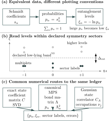
An entanglement-spectrum ledger. Panel (a) separates Schmidt coefficients $s_\alpha$, normalized probabilities $p_\alpha=s_\alpha^2$, and energy-like levels $\xi_\alpha=-\ln p_\alpha$. Panel (b) illustrates a phase-specific low-lying band organized by subsystem charge $q_A$; the entanglement gap $\Delta_{\rm ent}$ is meaningful only after the low-level sector pattern has been declared. Panel (c) shows three common extraction routes. Every plot should retain sector labels, normalization checks, and numerical errors.

Ordered probabilities and ordered levels

For a finite spectrum, plot either

$$p_0 \geq p_1 \geq \cdots$$

or

$$\xi_0 \leq \xi_1 \leq \cdots.$$

A probability plot makes normalization and truncation tails visible. An energy plot spreads small probabilities and makes level counting easier.

Because

$$\xi_\alpha = -\ln p_\alpha,$$

relative errors transform as

$$\delta\xi_\alpha \simeq -\frac{\delta p_\alpha}{p_\alpha}.$$

Tiny probabilities therefore produce large and unstable entanglement-energy errors. High-lying levels are usually the least numerically reliable part of the plot.

Degeneracy

An exact $g$-fold level degeneracy means

$$p_\alpha = p_{\alpha+1} = \cdots = p_{\alpha+g-1}.$$

Possible origins include:

• an irreducible symmetry multiplet;
• a projective edge representation;
• independent maximally entangled pairs;
• a cat-state superposition;
• a tensor-product factor;
• a solvable fixed point;
• an accidental finite-size coincidence.

The eigenvalues alone do not distinguish these mechanisms. One must inspect the Schmidt states, their symmetry action, the partition, perturbation response, and size dependence.

For an approximate multiplet, report a splitting such as

$$\delta_{\mathrm{mult}} := \max_{\alpha\in M}\xi_\alpha - \min_{\alpha\in M}\xi_\alpha$$

together with the numerical uncertainty and system-size dependence.

Schmidt gap

One common probability-space definition is

$$\Delta_{\mathrm S} := p_0-p_1.$$

The corresponding first entanglement-energy spacing is

$$\delta_\xi := \xi_1-\xi_0 = \ln\frac{p_0}{p_1}.$$

They vanish at the same exact degeneracy but are not numerically equal. The literature uses “Schmidt gap” inconsistently, sometimes for a difference of Schmidt coefficients $s_0-s_1$. Always state the formula.

A Schmidt-gap closing can be a useful finite-size indicator near selected quantum critical points. It is not a universal order parameter for every transition and does not replace conventional scaling analysis.

Entanglement gap

In topological and conformal applications, one may identify a low-lying set $L$ with a predicted sector counting and a higher set $H$. A convenient finite-size definition is

$$\Delta_{\mathrm{ent}} := \min_{\beta\in H}\xi_\beta - \max_{\alpha\in L}\xi_\alpha.$$

This definition requires the sets $L$ and $H$ to be specified independently of the desired conclusion. A blank horizontal space in one plot is not enough.

A credible entanglement-gap claim reports:

• the partition and geometry;
• the sector quantum numbers;
• the expected low-level counting;
• the rule assigning levels to $L$ and $H$;
• system-size or circumference scaling;
• stability across a finite parameter interval;
• sensitivity to numerical truncation;
• whether a common energy shift was removed.

The physical system may remain in one phase while its entanglement Hamiltonian changes qualitatively. Consequently, an entanglement gap need not be universal throughout a physical phase.

Rank and tail weight

The Schmidt rank is

$$r = \operatorname{rank}\rho_A.$$

For a cutoff retaining the largest $\chi$ probabilities, define the discarded weight

$$\epsilon_{\mathrm{disc}}(\chi) := \sum_{\alpha>\chi}p_\alpha.$$

The normalized truncated Schmidt state has squared overlap

$$\left| \langle\Psi\vert\Psi_\chi\rangle \right|^2 = 1-\epsilon_{\mathrm{disc}}(\chi).$$

Two states with equal entropy can have very different $\epsilon_{\mathrm{disc}}(\chi)$. This is why the spectrum, rather than entropy alone, controls matrix-product truncation quality.

Level counting versus level spacing

Universal information, when present, often resides more robustly in:

• how many levels occur in each sector;
• which multiplets are forced by symmetry;
• how counting changes under flux or boundary conditions;
• whether a predicted tower persists with size.

The precise level spacings can be nonuniversal and geometry dependent. Fitting an effective velocity or temperature to entanglement energies requires a theory that fixes the relevant normalization.

Symmetry-Resolved Spectra

Additive Abelian charge

Suppose an additive conserved charge satisfies

$$Q = Q_A+Q_{\bar A}$$

and the pure state has fixed total charge $Q_{\mathrm{tot}}$. The Schmidt decomposition can be chosen as

$$\lvert\Psi_{Q_{\mathrm{tot}}}\rangle = \sum_{q,\alpha} s_{q\alpha}\, \lvert q,\alpha\rangle_A \lvert Q_{\mathrm{tot}}-q,\alpha\rangle_{\bar A}.$$

The reduced state commutes with the subsystem charge:

$$[\rho_A,Q_A] = 0.$$

Therefore,

$$\rho_A = \bigoplus_q p_q\,\sigma_{A,q},$$

where

$$p_q := \sum_\alpha p_{q\alpha}, \qquad \operatorname{Tr}\sigma_{A,q} = 1.$$

Within a sector with $p_q>0$,

$$\sigma_{A,q} = \sum_\alpha \frac{p_{q\alpha}}{p_q} \lvert q,\alpha\rangle \langle q,\alpha\rvert.$$

The entropy separates into charge uncertainty and within-sector entropy:

$$\begin{aligned} S(\rho_A) &= H(\{p_q\}) \\ &\quad + \sum_q p_q S(\sigma_{A,q}), \end{aligned}$$

with

$$H(\{p_q\}) = -\sum_q p_q\ln p_q.$$

A sector-resolved entanglement plot should show both $q$ and the level index within each block. Plotting every sector after independently shifting its lowest level to zero destroys the relative sector weights.

Several commuting charges

For commuting observables

$$Q_A^{(1)}, \ldots, Q_A^{(k)},$$

levels can be labeled by a charge vector

$$\mathbf q = \left( q_1,\ldots,q_k \right).$$

Examples include:

• particle number and momentum along a translation-invariant cut;
• total $S^z$ and lattice parity;
• particle number and orbital angular momentum in quantum Hall geometries.

Every label requires the corresponding symmetry to preserve both the state and the partition. A symmetry exchanging $A$ and $\bar A$ does not automatically block-diagonalize $\rho_A$ in the same way as an onsite charge.

Non-Abelian symmetry

If a compact non-Abelian symmetry acts consistently on the bipartition and the global state is invariant, the Schmidt space decomposes into irreducible representations:

$$\mathcal H_{\mathrm{Schmidt}} \simeq \bigoplus_\lambda \left( \mathbb C^{m_\lambda} \otimes V_\lambda \right).$$

Here $V_\lambda$ is an irrep of dimension $d_\lambda$ and $m_\lambda$ is a multiplicity space. Symmetry forces each eigenvalue associated with an irrep block to occur at least $d_\lambda$ times when the reduced operator acts trivially within $V_\lambda$.

This representation-theoretic degeneracy is not automatically topological. It may occur in an ordinary singlet. Conversely, a topological or symmetry-protected diagnosis may require the projective transformation law of the Schmidt vectors, not just their eigenvalue multiplicity.

Degenerate subspaces and gauge freedom

Within an exactly degenerate eigenspace, numerical diagonalization returns an arbitrary orthonormal basis. Individual Schmidt vectors can rotate as

$$\lvert\alpha\rangle \longmapsto \sum_{\beta\in M} W_{\beta\alpha} \lvert\beta\rangle,$$

with $W$ unitary on the multiplet $M$.

To identify symmetry content:

1. isolate the degenerate or quasi-degenerate subspace;
2. project the symmetry operators into it;
3. diagonalize commuting labels or analyze the representation matrices;
4. test stability against basis rotations and truncation;
5. report the multiplet, not arbitrary eigenvectors.

Comparing raw Schmidt vectors from two parameter values without fixing this gauge can create fake discontinuities.

Projective symmetry on Schmidt states

In a one-dimensional gapped symmetry-protected phase, symmetry can act on virtual edge or Schmidt states through matrices $V_g$ satisfying

$$V_gV_h = \omega(g,h)V_{gh}.$$

The phase factor $\omega(g,h)$ defines a projective representation. Under allowed gauge changes,

$$V_g \longmapsto e^{i\theta_g} X V_g X^{-1},$$

the cocycle $\omega$ changes by a coboundary, while its cohomology class can remain invariant.

Protected entanglement degeneracies may follow from the irreducible projective representation, provided:

• the protecting symmetry is preserved;
• the bulk remains gapped;
• the cut is compatible with the symmetry;
• the thermodynamic limit is controlled.

Eigenvalue degeneracy alone does not determine the projective class.

Benchmark Spectra

Product state

For

$$\lvert\Psi\rangle = \lvert a\rangle_A \otimes \lvert b\rangle_{\bar A},$$

the only nonzero probability is

$$p_0=1.$$

Hence

$$\xi_0=0, \qquad S_A=0.$$

Every orthogonal direction in $\mathcal H_A$ belongs to the kernel and has infinite raw entanglement energy.

One two-level Schmidt pair

Consider

$$\lvert\psi(\theta)\rangle = \cos\theta\, \lvert00\rangle + \sin\theta\, \lvert11\rangle,$$

with

$$0\leq\theta\leq\frac{\pi}{4}.$$

The probabilities are

$$p_0 = \cos^2\theta, \qquad p_1 = \sin^2\theta.$$

The raw entanglement energies are

$$\xi_0 = -2\ln(\cos\theta), \qquad \xi_1 = -2\ln(\sin\theta).$$

The probability and energy gaps are

$$\Delta_{\mathrm S} = \cos(2\theta)$$

and

$$\delta_\xi = 2\ln(\cot\theta).$$

At $\theta=\pi/4$, the spectrum is flat and both gaps vanish. As $\theta\to0$, the second probability vanishes and its raw entanglement energy diverges.

Flat spectrum of rank R

For

$$p_\alpha = \frac1R, \qquad \alpha=1,\ldots,R,$$

all finite entanglement energies equal

$$\xi_\alpha = \ln R.$$

Every Rényi entropy has the same value:

$$S_A^{(n)} = \ln R.$$

A shifted $H_E$ convention can place all these levels at zero. Flatness indicates maximal entanglement on the occupied Schmidt support, not necessarily maximal entanglement on the full subsystem Hilbert space.

Several Bell pairs crossing the cut

Let $N$ independent qudit Bell pairs cross the bipartition:

$$\lvert\Psi\rangle = \bigotimes_{j=1}^{N} \frac1{\sqrt q} \sum_{a=0}^{q-1} \lvert a\rangle_{A_j} \lvert a\rangle_{\bar A_j}.$$

The Schmidt rank is

$$R=q^N,$$

and the spectrum is flat:

$$p_\alpha = q^{-N}.$$

Thus

$$S_A = N\ln q.$$

The degeneracy is generated by independent pairs. It is not, by itself, evidence of intrinsic topological order.

GHZ cat state

For the $V$-qubit GHZ state,

$$\lvert\mathrm{GHZ}_V\rangle = \frac{ \lvert0\rangle^{\otimes V} + \lvert1\rangle^{\otimes V} }{\sqrt2},$$

every nontrivial spatial bipartition has

$$p_0=p_1=\frac12.$$

Its nonzero entanglement spectrum is the same as one Bell pair, even though its multipartite correlations, local-unitary structure, and response to perturbations are different.

This example proves that a spectrum from one cut does not provide a complete classification of the global state.

AKLT half-chain benchmark

At the Affleck–Kennedy–Lieb–Tasaki fixed point, a cut through an infinite spin-1 chain exposes a virtual spin-$1/2$ degree of freedom. The half-chain spectrum has a twofold structure,

$$p_0=p_1=\frac12,$$

in the idealized fixed-point setting.

The same probability pair appeared for a Bell pair and a GHZ state. The additional SPT information lies in:

• how the Schmidt doublet transforms under the protecting symmetry;
• robustness under symmetry-preserving, gap-preserving deformations;
• lifting under appropriate symmetry breaking;
• finite-size convergence toward the half-infinite limit.

For a finite interval there are two entanglement cuts and therefore two virtual edges. The low spectrum can approach a four-state structure with splittings controlled by their effective coupling. Half-chain and finite-interval multiplicities should not be conflated.

Free-Fermion Correlation-Matrix Construction

Number-conserving Gaussian state

Consider fermionic modes $c_i$ and a Gaussian state that conserves particle number. For sites or orbitals in $A$, define the restricted one-body correlation matrix

$$(C_A)_{ij} := \langle c_i^\dagger c_j\rangle, \qquad i,j\in A.$$

It is Hermitian and satisfies

$$0 \leq C_A \leq I.$$

Diagonalize it as

$$C_A = U \operatorname{diag} \left( \nu_1,\ldots,\nu_{N_A} \right) U^\dagger,$$

where

$$0\leq\nu_j\leq1.$$

Define subsystem modes

$$f_j := \sum_{i\in A} U_{ij}^*c_i.$$

The reduced density operator factorizes over these entanglement modes:

$$\rho_A = \bigotimes_{j=1}^{N_A} \left[ (1-\nu_j)(1-n_j) + \nu_j n_j \right],$$

with

$$n_j := f_j^\dagger f_j.$$

This is a statement about Gaussian states. Matching only the two-point matrix does not determine the reduced state of a generic interacting, non-Gaussian system.

Single-particle entanglement Hamiltonian

The same reduced state can be written

$$\rho_A = \frac1{Z_E} \exp \left( -\sum_j\epsilon_j n_j \right),$$

where

$$\epsilon_j = \ln \frac{1-\nu_j}{\nu_j}.$$

In the original subsystem basis,

$$H_E = \sum_{i,j\in A} h_{ij}c_i^\dagger c_j,$$

with the one-body matrix

$$h = \ln \left[ (I-C_A)C_A^{-1} \right]$$

on eigenmodes with $0<\nu_j<1$.

The $\epsilon_j$ are single-particle entanglement energies. They can be negative because a common many-body normalization shift has not yet been added. They are not the raw nonnegative values $-\ln p_{\mathbf n}$.

Building the many-body spectrum

For an occupation pattern

$$\mathbf n = (n_1,\ldots,n_{N_A}), \qquad n_j\in\{0,1\},$$

the probability is

$$p_{\mathbf n} = \prod_{j=1}^{N_A} \nu_j^{n_j} (1-\nu_j)^{1-n_j}.$$

The raw many-body entanglement energy is

$$\begin{aligned} \xi_{\mathbf n} &= -\ln p_{\mathbf n} \\ &= -\sum_j n_j\ln\nu_j \\ &\quad -\sum_j (1-n_j)\ln(1-\nu_j). \end{aligned}$$

Equivalently,

$$\xi_{\mathbf n} = \ln Z_E + \sum_j n_j\epsilon_j.$$

The many-body spectrum therefore consists of all occupation sums of the single-particle levels, plus one common normalization shift.

Entropy from correlation eigenvalues

The entropy is additive over entanglement modes:

$$S_A = \sum_j h_2(\nu_j),$$

where

$$h_2(\nu) := -\nu\ln\nu - (1-\nu)\ln(1-\nu).$$

A mode with

$$\nu_j=\frac12$$

has

$$\epsilon_j=0$$

and contributes $\ln2$. Such a zero single-particle entanglement energy often accompanies an edge-like or cut mode in free-fermion topological models, but its interpretation still depends on symmetry, geometry, and finite-size stability.

A mode with $\nu_j=0$ or $1$ is deterministic and contributes no entropy. The corresponding $\epsilon_j$ diverges, but the normalized many-body probability of the allowed occupation remains finite.

Pairing and bosonic variants

For superconducting Gaussian states, anomalous correlators

$$\langle c_i c_j\rangle$$

are nonzero. The number-conserving matrix $C_A$ is then insufficient; one diagonalizes a Nambu covariance matrix or a Majorana correlation matrix.

Gaussian bosonic states require symplectic eigenvalues of a covariance matrix and careful treatment of unbounded local Hilbert spaces. Those constructions share the quadratic entanglement-Hamiltonian idea but use different spectra and stability conditions.

Numerical Extraction

Exact diagonalization and wavefunction reshaping

For a pure state expanded in product bases,

$$\lvert\Psi\rangle = \sum_{i=1}^{d_A} \sum_{\mu=1}^{d_{\bar A}} C_{i\mu} \lvert i\rangle_A \lvert\mu\rangle_{\bar A},$$

the reduced matrix is

$$\rho_A = CC^\dagger.$$

If

$$C = U\Sigma V^\dagger$$

is a singular-value decomposition, then

$$s_\alpha = \Sigma_{\alpha\alpha}, \qquad p_\alpha = s_\alpha^2.$$

Computing the singular values of $C$ is usually preferable to explicitly forming $CC^\dagger$:

• it avoids squaring the condition number;
• it preserves positivity more reliably;
• it returns Schmidt vectors on both sides;
• it can target only the largest singular values.

The coefficient matrix depends on the tensor-product ordering. Before reshaping a many-body vector, verify the basis convention with a product-state and Bell-pair test.

Symmetry-blocked exact diagonalization

If total charge is fixed, arrange $C$ into compatible blocks:

$$C = \bigoplus_q C_q.$$

An SVD of each block yields $p_{q\alpha}$ directly. This:

• reduces memory;
• preserves exact labels;
• avoids numerical mixing of degenerate sectors;
• makes sector weights $p_q$ explicit.

The singular values from all blocks must be combined before global normalization checks or entropy calculation.

Matrix-product states

At a canonical MPS bond cut,

$$\lvert\Psi\rangle = \sum_{\alpha=1}^{\chi} \Lambda_\alpha \lvert L_\alpha\rangle \lvert R_\alpha\rangle,$$

with orthonormal Schmidt states and

$$\sum_\alpha\Lambda_\alpha^2=1.$$

Therefore,

$$p_\alpha = \Lambda_\alpha^2.$$

The bond entanglement spectrum is available without constructing an exponentially large reduced density matrix.

For a finite interval inside an infinite chain there are two cuts. The interval spectrum is not generally the spectrum of one MPS bond. It must be obtained from the interval transfer operator or an explicit reduced-state contraction.

Truncation and discarded weight

Keeping the largest $\chi$ Schmidt coefficients gives

$$\epsilon_{\mathrm{disc}} = 1- \sum_{\alpha=1}^{\chi}p_\alpha.$$

A reported spectrum should state:

• the maximum bond dimension;
• the discarded weight at the cut;
• the canonicalization tolerance;
• whether symmetry multiplets were truncated together;
• the smallest trusted probability;
• convergence under larger $\chi$.

Cutting through part of a symmetry multiplet can introduce artificial level splitting and even break the represented symmetry.

Transfer matrices and infinite systems

For a translation-invariant infinite MPS, the transfer matrix controls:

• canonical fixed points;
• normalization;
• correlation length;
• finite-interval reduced states;
• coupling between virtual edges.

If the transfer matrix has leading eigenvalues

$$\lambda_0=1, \qquad \lvert\lambda_1\rvert<1,$$

the correlation length is

$$\xi_{\mathrm{corr}} = -\frac1{\ln\lvert\lambda_1\rvert}.$$

For an interval of length $\ell$ in a gapped injective MPS, interactions between its two virtual entanglement edges are typically suppressed on scales set by

$$e^{-\ell/\xi_{\mathrm{corr}}}.$$

This explains why finite-interval multiplets may approach their asymptotic degeneracy exponentially rather than being exactly degenerate at small $\ell$.

Sparse and stochastic methods

For large reduced states, one may use:

• iterative eigensolvers for the largest $p_\alpha$;
• randomized or matrix-free singular-value methods;
• tensor-network boundary contractions;
• replica or moment methods;
• quantum Monte Carlo estimators in special sign-free settings.

Moments such as $\operatorname{Tr}\rho_A^n$ do not automatically resolve individual fine levels. Reconstructing a broad spectrum from noisy moments is an ill-conditioned inverse problem and requires explicit regularization and uncertainty analysis.

Topological and Boundary Structure

Partition comes first

Different partitions expose different structures:

• real-space cut: probes a spatial entanglement boundary;
• orbital cut: partitions a chosen one-particle orbital basis;
• particle cut: traces out a subset of indistinguishable particles;
• momentum cut: partitions modes in reciprocal space;
• internal cut: separates spin, layer, species, or other internal labels.

Two partitions of the same wavefunction need not have similar spectra. The phrase “the entanglement spectrum of the phase” is incomplete without the partition.

Li–Haldane orbital spectrum

Li and Haldane introduced the entanglement-spectrum viewpoint in fractional quantum Hall trial and Coulomb states using an orbital partition. In their examples:

• low-lying entanglement levels had characteristic angular-momentum counting;
• the counting matched the expected edge conformal field theory;
• a higher generic set could be separated by an entanglement gap.

The safe conclusion is model and geometry specific. It rests on the conjunction of:

• appropriate low-level counting;
• controlled finite-size scaling;
• independent evidence for the phase assignment.

A visible entanglement gap by itself does not imply topological order.

Orbital, particle, and real-space spectra can reveal complementary edge or bulk-quasihole information. Their level counts should not be compared as though the cuts were interchangeable.

Entanglement edge versus physical edge

An entanglement cut creates an interface in the wavefunction but does not physically terminate the Hamiltonian. Under controlled conditions, the low entanglement spectrum can correspond to a boundary theory:

• free topological insulators and superconductors admit exact relations involving a spectrally flattened Hamiltonian;
• selected gapped topological states with chiral edge conformal theories admit a boundary-CFT relation;
• projected entangled-pair states map bulk reduced states to operators on virtual boundaries.

These results differ in hypotheses and construction. None implies the unrestricted identity

$$H_E = H_{\mathrm{physical\ edge}}.$$

The physical edge depends on its termination and local interactions. The entanglement boundary depends on the state, cut, normalization, and virtual representation.

One-dimensional symmetry-protected phases

For a half-infinite one-dimensional gapped state, the entanglement cut exposes one virtual edge. In the Haldane phase, Pollmann, Turner, Berg, and Oshikawa identified a double structure protected by specified symmetries, including suitable dihedral spin rotations, time reversal, or bond-centered inversion.

The evidence package is:

1. a gapped bulk phase;
2. a declared protecting symmetry;
3. Schmidt states carrying the appropriate projective or protected action;
4. stable multiplet structure under symmetry-preserving perturbations;
5. lifting or trivialization when the relevant protection is removed;
6. controlled finite-size or bond-dimension convergence.

A twofold spectrum in one finite chain is insufficient.

Intrinsic topological order

In two-dimensional intrinsically topological phases, reduced-state structure can reflect:

• boundary superselection sectors;
• anyon flux through a cylinder;
• edge-theory level counting;
• topological constraints on virtual boundary operators.

However, intrinsic topological order is not defined by an entanglement-spectrum pattern alone. The canonical evidence also includes local indistinguishability, topology-dependent ground sectors, loop operators, anyonic fusion and braiding, and stability under local perturbations.

Topological Entanglement Entropy Preview owns the universal constant term and selected area-law combinations. The entanglement spectrum instead retains a much larger, more partition-sensitive set of reduced-state data.

Why degeneracy alone is weak evidence

The following can all produce low-level degeneracy:

• symmetry multiplets in a trivial singlet;
• GHZ-type symmetry-breaking cat states;
• independent Bell pairs;
• SPT virtual edges;
• free-fermion boundary zero modes;
• intrinsic topological sectors;
• exact fixed-point tensors;
• accidental finite-size crossings.

To identify the mechanism, ask:

• Which symmetry acts on the Schmidt space?
• Which partition and boundary geometry were used?
• How does the splitting scale?
• What perturbations lift it?
• Which independent bulk diagnostic agrees?

Non-universality within a phase

The complete entanglement spectrum is generally not universal. Even while a physical Hamiltonian remains in one gapped phase:

• high levels can change strongly;
• entanglement gaps can close or reopen;
• the entanglement Hamiltonian can undergo its own spectral rearrangement;
• a different cut can change the apparent boundary theory;
• short-distance unitary circuits near the cut can reshape the spectrum.

Robust claims should target structures protected by a theorem, symmetry representation, topological sector, or controlled low-energy limit. “The spectra look alike” is suggestive evidence, not a phase equivalence proof.

Critical and Excited States

One-dimensional conformal criticality

For a real-space interval in selected one-dimensional critical ground states, the low entanglement spectrum can organize into towers associated with a boundary conformal field theory. This can reveal operator content beyond the central charge extracted from entropy scaling.

The correspondence depends on:

• interval geometry and boundary conditions;
• the ultraviolet regularization;
• the conformal mapping;
• which symmetry sectors are resolved;
• finite-size corrections;
• how entanglement energies are shifted and rescaled.

Tower counting can be more meaningful than raw spacings. A finite set of approximately equally spaced levels is not by itself proof of conformal invariance.

Critical closing and the Schmidt gap

Near selected quantum critical points, the largest probabilities can reorganize and the Schmidt gap can close with finite-size scaling. A careful analysis compares

$$\Delta_{\mathrm S}(g,L)$$

over several sizes $L$ and couplings $g$, using the same partition and symmetry sector.

The critical point, exponent, and scaling function should be checked against:

• the physical gap;
• correlation length;
• conventional order parameters when present;
• entanglement entropy scaling;
• boundary-condition dependence.

An isolated crossing of $p_0$ and $p_1$ can be symmetry generated or accidental.

Chaotic eigenstates and random states

Highly excited chaotic eigenstates and Haar-random states often have dense, volume-law spectra. Their reduced eigenvalues can be compared with energy-shell or random-matrix benchmarks, but the reference ensemble matters.

A full-Hilbert-space Haar state and a finite-energy eigenstate differ in:

• accessible entropy density;
• conserved charges;
• energy-shell constraints;
• finite-subsystem-fraction corrections;
• correlations among eigenvalues.

Volume Laws owns those distinctions. Here the lesson is narrower: equal entropy density does not imply equal entanglement spectra.

Quench dynamics

After a global quench, both probabilities and Schmidt vectors evolve:

$$p_\alpha \longrightarrow p_\alpha(t).$$

Tracking only

$$S_A(t)$$

can hide:

• level crossings;
• symmetry-sector transport;
• delayed convergence of the spectral tail;
• numerical saturation at finite bond dimension;
• persistent nonthermal low-level structure.

Dynamic entanglement spectra are especially sensitive to truncation because newly generated small probabilities become high entanglement levels before they contribute strongly to entropy.

A Reliable Numerical Workflow

Step 1: write the state ledger

State:

• pure or mixed global state;
• ground, eigenstate, thermal, quench, or trajectory state;
• Hamiltonian parameters and symmetry sector;
• normalization and numerical representation.

For a mixed global state, explain why the reduced spectrum is being called entanglement data, if it is.

Step 2: write the partition ledger

Specify:

• real-space, orbital, particle, momentum, or internal cut;
• subsystem size and total size;
• number of connected entanglement boundaries;
• boundary conditions and topology;
• basis or orbital convention;
• gauge or algebra convention when factorization is subtle.

Changing the cut changes the observable.

Step 3: extract without losing structure

Prefer:

• SVD of the wavefunction coefficient matrix for a pure exact state;
• canonical bond singular values for a one-cut MPS;
• symmetry-blocked decompositions when charges are exact;
• covariance-matrix methods only for Gaussian states.

Retain eigenvectors or projected symmetry matrices when the claim involves symmetry representations.

Step 4: validate the probabilities

Check

$$\sum_\alpha p_\alpha = 1$$

within a reported tolerance and verify

$$p_\alpha \geq 0.$$

Record:

$$\epsilon_{\mathrm{trace}} := \left| 1-\sum_\alpha p_\alpha \right|$$

and

$$\epsilon_{\mathrm{neg}} := \sum_{p_\alpha<0} \lvert p_\alpha\rvert.$$

Do not simply discard negative numerical eigenvalues before documenting their total weight.

Step 5: choose the plotted convention

Declare whether the vertical axis is:

$$p_\alpha, \qquad -\ln p_\alpha, \qquad \text{or} \qquad -\ln(p_\alpha/p_0).$$

If each sector is shifted separately, say so and preserve a separate plot of the sector weights.

Step 6: attach quantum numbers

For every displayed level, retain all exact labels supported by the state and cut. If degeneracies are central, analyze symmetry within the full multiplet rather than labeling arbitrary eigenvectors.

Step 7: perform convergence tests

Vary:

• total size;
• subsystem size or aspect ratio;
• bond dimension;
• eigensolver tolerance;
• probability cutoff;
• symmetry-preserving perturbations;
• boundary conditions;
• parameter values inside the proposed phase.

Plot splitting, gap, and discarded weight against the relevant size variable. A single visually clean spectrum is an illustration, not an asymptotic result.

Step 8: reconstruct scalar checks

From the retained probabilities, recompute:

$$S_A = -\sum_\alpha p_\alpha\ln p_\alpha$$

and selected moments:

$$\operatorname{Tr}\rho_A^n = \sum_\alpha p_\alpha^n.$$

Compare them with independently computed entropies when available. Disagreement can expose missing sectors, wrong normalization, basis-ordering mistakes, or truncation.

Step 9: match the claim to the evidence

Use language such as:

• “the half-chain spectrum forms symmetry-labeled doublets within the numerical tolerance”;
• “the low orbital levels have the predicted counting over the sizes studied”;
• “an entanglement gap defined by this counting remains positive on the available circumferences”;
• “the full high-level spectrum is nonuniversal and not used in the phase claim.”

Avoid:

• “the spectrum proves topology”;
• “the entanglement Hamiltonian is the edge Hamiltonian”;
• “two equal entropies imply the same spectrum”;
• “all small levels are converged.”

Common Mistakes

• Not defining “Schmidt value.” State whether it means $s_\alpha$ or $p_\alpha=s_\alpha^2$.
• Mixing raw and shifted energies. Absolute $\xi_\alpha=-\ln p_\alpha$ and $\xi_\alpha-\xi_0$ have different information.
• Taking the logarithm of numerical noise. Negative and tiny eigenvalues require an error ledger and cutoff.
• Calling a mixed-state subsystem spectrum entanglement. A maximally mixed product state has a flat reduced spectrum and no correlations.
• Reading every degeneracy as topological. Symmetry, cat states, Bell pairs, and accidental crossings can all generate degeneracy.
• Ignoring quantum numbers. Level counting without sector labels is often meaningless.
• Shifting every sector independently without reporting weights. This erases physically relevant charge probabilities.
• Equating the Schmidt gap with an entanglement-energy gap. $p_0-p_1$ and $\ln(p_0/p_1)$ are distinct.
• Equating the entanglement gap with the physical gap. They arise from different operators.
• Assuming $K_A=\beta H_A$. Exact modular Hamiltonians are generally state and boundary dependent.
• Using one finite-size blank region as an entanglement gap. Define the low set and perform scaling.
• Comparing different cuts as though they were the same observable. Orbital, particle, momentum, and real-space partitions are inequivalent.
• Applying the correlation-matrix formula to an interacting non-Gaussian state. Two-point data then do not determine $\rho_A$.
• Using one MPS bond for a finite interval. An interval usually has two entanglement boundaries.
• Cutting a symmetry multiplet during truncation. This creates artificial splitting and symmetry breaking.
• Comparing Schmidt eigenvectors without fixing degenerate-subspace gauge. Arbitrary rotations can look like physical discontinuities.
• Treating the full spectrum as universal within a phase. Short-distance unitaries near the cut can reshape it.
• Using the spectrum as a stand-alone classifier. Combine it with gaps, symmetries, correlations, response, and phase-specific diagnostics.

Exercises

1. Two-level spectrum and two gap conventions

For

$$\lvert\psi\rangle = \frac{\sqrt3}{2}\lvert00\rangle + \frac12\lvert11\rangle,$$

find:

1. the Schmidt probabilities;
2. the raw entanglement energies;
3. the von Neumann entropy;
4. the probability Schmidt gap $p_0-p_1$;
5. the first entanglement-energy spacing $\xi_1-\xi_0$.

Solution

The Schmidt coefficients are

$$s_0 = \frac{\sqrt3}{2}, \qquad s_1 = \frac12.$$

Therefore,

$$p_0 = \frac34, \qquad p_1 = \frac14.$$

The raw levels are

$$\xi_0 = -\ln\frac34 = \ln\frac43$$

and

$$\xi_1 = -\ln\frac14 = \ln4.$$

The entropy is

$$\begin{aligned} S_A &= -\frac34\ln\frac34 - \frac14\ln\frac14 \\ &= \ln4 - \frac34\ln3. \end{aligned}$$

The probability gap is

$$\Delta_{\mathrm S} = \frac34-\frac14 = \frac12.$$

The energy spacing is

$$\begin{aligned} \delta_\xi &= \ln4-\ln\frac43 \\ &= \ln3. \end{aligned}$$

The two gaps diagnose the same exact two-level degeneracy but use different nonlinear coordinates.

2. Fixing the entanglement-Hamiltonian shift

An unnormalized entanglement Hamiltonian has three eigenvalues

$$\varepsilon \in \left\{ 0,\ln2,\ln6 \right\}.$$

Compute $Z_E$, the normalized probabilities, and the raw entanglement energies.

Solution

The Boltzmann-like weights are

$$\left\{ 1,\frac12,\frac16 \right\}.$$

Thus

$$Z_E = 1+\frac12+\frac16 = \frac53.$$

After normalization,

$$\{p_\alpha\} = \left\{ \frac35, \frac3{10}, \frac1{10} \right\}.$$

The raw levels are

$$\{\xi_\alpha\} = \left\{ \ln\frac53, \ln\frac{10}{3}, \ln10 \right\}.$$

Equivalently,

$$\xi_\alpha = \varepsilon_\alpha + \ln Z_E.$$

Adding any constant to all $\varepsilon_\alpha$ changes $Z_E$ but leaves the normalized probabilities and raw $\xi_\alpha$ unchanged.

3. Symmetry-sector entropy decomposition

A reduced state has two charge sectors. Their weights and conditional spectra are

$$p_{q=0} = \frac34, \qquad \operatorname{spec}(\sigma_{A,0}) = \left\{ \frac23,\frac13 \right\},$$

and

$$p_{q=1} = \frac14, \qquad \operatorname{spec}(\sigma_{A,1}) = \{1\}.$$

1. Find the full spectrum of $\rho_A$.
2. Verify

$$S(\rho_A) = H(\{p_q\}) + \sum_q p_qS(\sigma_{A,q}).$$

Solution

Multiplying sector weights by conditional probabilities gives

$$\operatorname{spec}(\rho_A) = \left\{ \frac12,\frac14,\frac14 \right\}.$$

Therefore,

$$\begin{aligned} S(\rho_A) &= -\frac12\ln\frac12 - 2\left(\frac14\ln\frac14\right) \\ &= \frac32\ln2. \end{aligned}$$

The charge entropy is

$$H(\{p_q\}) = -\frac34\ln\frac34 - \frac14\ln\frac14.$$

Only the $q=0$ sector has internal entropy:

$$S(\sigma_{A,0}) = -\frac23\ln\frac23 - \frac13\ln\frac13.$$

Hence

$$\begin{aligned} H(\{p_q\}) &+ \frac34S(\sigma_{A,0}) \\ &= \frac32\ln2, \end{aligned}$$

as required. The $q=1$ sector is pure and contributes no within-sector entropy.

4. Two Gaussian entanglement modes

A number-conserving fermionic Gaussian reduced state has correlation eigenvalues

$$\nu_1 = \frac34, \qquad \nu_2 = \frac14.$$

1. Find all four many-body probabilities.
2. Find the single-particle entanglement energies.
3. Find the entropy.

Solution

For occupations $(n_1,n_2)$,

$$p_{n_1n_2} = \nu_1^{n_1}(1-\nu_1)^{1-n_1} \nu_2^{n_2}(1-\nu_2)^{1-n_2}.$$

Thus

$$\begin{array}{c|c} (n_1,n_2) & p_{n_1n_2} \\ \hline (0,0) & 3/16 \\ (1,0) & 9/16 \\ (0,1) & 1/16 \\ (1,1) & 3/16 \end{array}$$

and the probabilities sum to one.

The single-particle entanglement energies are

$$\epsilon_1 = \ln\frac{1/4}{3/4} = -\ln3$$

and

$$\epsilon_2 = \ln\frac{3/4}{1/4} = \ln3.$$

The entropy is

$$\begin{aligned} S_A &= h_2\!\left(\frac34\right) + h_2\!\left(\frac14\right) \\ &= 2\ln4 - \frac32\ln3. \end{aligned}$$

The negative value of $\epsilon_1$ is harmless: these are shifted single-particle levels. Every raw many-body value $-\ln p_{n_1n_2}$ is nonnegative.

5. MPS truncation ledger

Across one MPS bond, the Schmidt probabilities are

$$\left\{ 0.55,\, 0.25,\, 0.12,\, 0.05,\, 0.03 \right\}.$$

If only $\chi=3$ values are retained:

1. find the discarded weight;
2. find the squared overlap with the normalized truncated state;
3. find the normalized retained probabilities.

Solution

The retained weight is

$$w_\chi = 0.55+0.25+0.12 = 0.92.$$

Therefore,

$$\epsilon_{\mathrm{disc}} = 1-w_\chi = 0.08.$$

For Schmidt truncation, the normalized truncated state’s squared overlap with the original state is

$$\left| \langle\Psi\vert\Psi_\chi\rangle \right|^2 = w_\chi = 0.92.$$

The retained probabilities must be renormalized:

$$\left\{ \frac{55}{92}, \frac{25}{92}, \frac{12}{92} \right\}.$$

Computing entropy from the unnormalized retained values would mix physical entanglement with numerical norm loss.

6. Same eigenvalues, different physics

A Bell pair, a nontrivial cut of an $N$-qubit GHZ state, and an ideal AKLT half-chain can each have the nonzero probability spectrum

$$\left\{ \frac12,\frac12 \right\}.$$

List at least four additional diagnostics needed to distinguish their physical structures.

Solution

Useful diagnostics include:

1. Schmidt-state symmetry action. The AKLT doublet carries protected virtual-edge structure under specified symmetries.
2. Other bipartitions. GHZ retains a two-level spectrum for every nontrivial site partition, while one Bell pair is localized to its paired degrees of freedom.
3. Local correlations and reduced states. GHZ has cat-state correlations and fragile coherence; a Bell pair has localized two-body entanglement.
4. Perturbation response. SPT structure is stable only under its protecting symmetry and a bulk gap; GHZ degeneracy is tied to symmetry-breaking cat structure.
5. System-size scaling. Virtual-edge splittings, cat-state tunneling, and isolated-pair structure scale differently.
6. Boundary and geometry dependence. A finite AKLT interval has two virtual edges, unlike a half-chain.
7. Bulk diagnostics. Correlation length, string order, gap, and phase path provide independent evidence.

The example illustrates that eigenvalues from one cut do not specify the Schmidt vectors, symmetry representation, or global state.

7. A declared entanglement gap

A sector-resolved calculation identifies low levels

$$L = \{0,0.2,0.2,0.5\}$$

and higher levels

$$H = \{1.4,1.7\}.$$

1. Compute the entanglement gap.
2. Show that a common additive shift does not change it.
3. Explain why shifting different symmetry sectors independently can obstruct the comparison.

Solution

By definition,

$$\begin{aligned} \Delta_{\mathrm{ent}} &= \min H-\max L \\ &= 1.4-0.5 \\ &= 0.9. \end{aligned}$$

Under a common shift $\xi\mapsto\xi+c$,

$$\begin{aligned} \Delta_{\mathrm{ent}}' &= (\min H+c) - (\max L+c) \\ &= \Delta_{\mathrm{ent}}. \end{aligned}$$

If each charge sector is shifted by a different constant, relative positions between sectors change. One can no longer tell which sector contains the globally lowest level or how sector probabilities compare. Sectorwise shifting is useful for internal tower counting only when an unshifted spectrum and the sector weights are also retained.

8. Audit a topological-spectrum claim

An exact-diagonalization study of one finite fractional quantum Hall cluster shows low orbital-entanglement levels with the expected edge counting and a visible blank region above them. The authors conclude that the state has definitively established topological order.

What additional evidence is needed before making a strong claim?

Solution

The observed counting is useful evidence, but the conclusion is too strong. A controlled analysis should add:

• several system sizes or circumferences;
• a precise rule defining the low-level set and entanglement gap;
• sector-resolved counting and finite-size corrections;
• stability over a finite Hamiltonian-parameter interval;
• convergence with Hilbert-space truncation and eigensolver tolerance;
• comparison with real-space or particle cuts where appropriate;
• physical bulk-gap and ground-sector scaling;
• independent topological diagnostics such as flux response, modular data, quasiparticle sectors, or local indistinguishability;
• tests against symmetry breaking, accidental degeneracy, and competing phases.

Even a stable entanglement gap is not a universal definition of topological order. The strongest conclusion comes from agreement among phase-specific spectral, bulk, and response evidence.

Summary

For a pure bipartite state,

$$\lvert\Psi\rangle = \sum_\alpha s_\alpha \lvert\alpha\rangle_A \lvert\alpha\rangle_{\bar A},$$

the Schmidt probabilities are

$$p_\alpha=s_\alpha^2, \qquad \sum_\alpha p_\alpha=1.$$

The energy-like spectrum is

$$\xi_\alpha=-\ln p_\alpha.$$

The normalized modular Hamiltonian

$$K_A=-\ln\rho_A$$

has eigenvalues $\xi_\alpha$. An alternative $H_E$ defined through

$$\rho_A = \frac{e^{-H_E}}{Z_E}$$

is shift ambiguous.

Entropy and Rényi moments are spectral summaries:

$$\begin{aligned} S_A &= \sum_\alpha p_\alpha\xi_\alpha, \\ \operatorname{Tr}\rho_A^n &= \sum_\alpha e^{-n\xi_\alpha}. \end{aligned}$$

Symmetries organize the spectrum into sectors and multiplets. For an additive charge,

$$\rho_A = \bigoplus_q p_q\sigma_{A,q},$$

and

$$S(\rho_A) = H(\{p_q\}) + \sum_qp_qS(\sigma_{A,q}).$$

For number-conserving fermionic Gaussian states, the eigenvalues $\nu_j$ of the restricted correlation matrix determine the complete many-body spectrum:

$$p_{\mathbf n} = \prod_j \nu_j^{n_j} (1-\nu_j)^{1-n_j}.$$

The entanglement spectrum can expose symmetry representations, truncation tails, boundary-like counting, and phase-specific low-level structure. Its interpretation remains conditional on the state, partition, symmetry, geometry, normalization, and finite-size limit. Degeneracy or an apparent entanglement gap is evidence to be explained, not a self-interpreting proof.

References

1. I. Peschel, “Calculation of reduced density matrices from correlation functions,” Journal of Physics A: Mathematical and General 36, L205–L208 (2003). doi:10.1088/0305-4470/36/14/101
2. P. Calabrese and A. Lefevre, “Entanglement spectrum in one-dimensional systems,” Physical Review A 78, 032329 (2008). doi:10.1103/PhysRevA.78.032329
3. H. Li and F. D. M. Haldane, “Entanglement spectrum as a generalization of entanglement entropy: Identification of topological order in non-Abelian fractional quantum Hall effect states,” Physical Review Letters 101, 010504 (2008). doi:10.1103/PhysRevLett.101.010504
4. I. Peschel and V. Eisler, “Reduced density matrices and entanglement entropy in free lattice models,” Journal of Physics A: Mathematical and Theoretical 42, 504003 (2009). doi:10.1088/1751-8113/42/50/504003
5. F. Pollmann, A. M. Turner, E. Berg, and M. Oshikawa, “Entanglement spectrum of a topological phase in one dimension,” Physical Review B 81, 064439 (2010). doi:10.1103/PhysRevB.81.064439
6. L. Fidkowski, “Entanglement spectrum of topological insulators and superconductors,” Physical Review Letters 104, 130502 (2010). doi:10.1103/PhysRevLett.104.130502
7. R. Thomale, A. Sterdyniak, N. Regnault, and B. A. Bernevig, “Entanglement gap and a new principle of adiabatic continuity,” Physical Review Letters 104, 180502 (2010). doi:10.1103/PhysRevLett.104.180502
8. A. M. Turner, F. Pollmann, and E. Berg, “Topological phases of one-dimensional fermions: An entanglement point of view,” Physical Review B 83, 075102 (2011). doi:10.1103/PhysRevB.83.075102
9. A. Sterdyniak, N. Regnault, and B. A. Bernevig, “Extracting excitations from model state entanglement,” Physical Review Letters 106, 100405 (2011). doi:10.1103/PhysRevLett.106.100405
10. J. I. Cirac, D. Poilblanc, N. Schuch, and F. Verstraete, “Entanglement spectrum and boundary theories with projected entangled-pair states,” Physical Review B 83, 245134 (2011). doi:10.1103/PhysRevB.83.245134
11. A. Chandran, M. Hermanns, N. Regnault, and B. A. Bernevig, “Bulk-edge correspondence in entanglement spectra,” Physical Review B 84, 205136 (2011). doi:10.1103/PhysRevB.84.205136
12. U. Schollwöck, “The density-matrix renormalization group in the age of matrix product states,” Annals of Physics 326, 96–192 (2011). doi:10.1016/j.aop.2010.09.012
13. X.-L. Qi, H. Katsura, and A. W. W. Ludwig, “General relationship between the entanglement spectrum and the edge state spectrum of topological quantum states,” Physical Review Letters 108, 196402 (2012). doi:10.1103/PhysRevLett.108.196402
14. V. Alba, M. Haque, and A. M. Läuchli, “Boundary-locality and perturbative structure of entanglement spectra in gapped systems,” Physical Review Letters 108, 227201 (2012). doi:10.1103/PhysRevLett.108.227201
15. G. De Chiara, L. Lepori, M. Lewenstein, and A. Sanpera, “Entanglement spectrum, critical exponents, and order parameters in quantum spin chains,” Physical Review Letters 109, 237208 (2012). doi:10.1103/PhysRevLett.109.237208
16. M. P. Zaletel, R. S. K. Mong, and F. Pollmann, “Topological characterization of fractional quantum Hall ground states from microscopic Hamiltonians,” Physical Review Letters 110, 236801 (2013). doi:10.1103/PhysRevLett.110.236801
17. A. Chandran, V. Khemani, and S. L. Sondhi, “How universal is the entanglement spectrum?,” Physical Review Letters 113, 060501 (2014). doi:10.1103/PhysRevLett.113.060501
18. N. Laflorencie, “Quantum entanglement in condensed matter systems,” Physics Reports 646, 1–59 (2016). doi:10.1016/j.physrep.2016.06.008
19. M. Dalmonte, V. Eisler, M. Falconi, and B. Vermersch, “Entanglement Hamiltonians: From field theory to lattice models and experiments,” Annalen der Physik 534, 2200064 (2022). doi:10.1002/andp.202200064

Cross-Links

• Symmetry-Protected Topological Phases — projective Schmidt actions, stable equivalence, boundary anomalies, and the distinction from intrinsic topological order.

• Topological Order — minimally entangled sectors, modular data, total quantum dimension, and the evidence needed beyond one spectral pattern.

• Bulk–Boundary Correspondence — the physical-boundary index theorem and the precise distinction among edge, Wilson-loop, and entanglement spectral flow.

• Many-Body Entanglement Overview

• Entanglement Entropy in Many-Body Systems

• Area Laws

• Volume Laws

• Tensor Networks Preview — Schmidt tails, bond dimensions, network cuts, and family-specific representation limits.

• Matrix Product States Preview — canonical bonds, transfer spectra, injectivity, and the direct extraction of Schmidt data.

• Thermal Entropy vs Entanglement Entropy

• Topological Order Preview

• Variational Many-Body States

• Schmidt Decomposition

• Reduced Density Operators

• Rényi Entropies

• Formula Sheet

• Entanglement in Many-Body Physics

• Entanglement in QFT Preview

• Symmetry-Protected Structure Preview

• Spectral Decomposition