Volume Laws

A volume law says that the leading entropy of a region grows in proportion to the number of degrees of freedom in its interior:

$$S_A = s_{\mathrm{vol}}V_A + o(V_A),$$

with a nonzero entropy density $s_{\mathrm{vol}}$. On a lattice, $V_A$ is the number of sites or unit cells in $A$. For a continuum theory, both $V_A$ and the entropy require a regulator and a declared subtraction scheme.

The formula is a scaling class, not a mechanism. It can describe:

• ordinary mixed-state entropy in a Gibbs ensemble;
• genuine bipartite entanglement in a Haar-random pure state;
• entanglement in a chaotic finite-energy-density eigenstate;
• entanglement generated dynamically after a global quench;
• nonthermal volume laws in integrable, constrained, or localized dynamics.

These cases may have the same small-region slope and radically different global states. A pure state obeys complement symmetry and returns to zero entropy when $A$ becomes the whole system. A mixed thermal state generally does not. A random vector in the full Hilbert space is nearly infinite-temperature locally, whereas an energy eigenstate is confined to an energy shell. A quench state acquires its volume law through time-dependent transport of quantum information.

The central task is therefore to identify not only

$$S_A\propto V_A,$$

but also:

$$\begin{gathered} \text{which density operator,} \\ \text{which state family,} \\ \text{which subsystem-fraction limit,} \\ \text{which conserved sector,} \\ \text{and which dynamical timescale.} \end{gathered}$$

Scope and Canonical Ownership

This page is the canonical home for many-body volume-law scaling. It owns:

• precise thermodynamic and finite-subsystem-fraction definitions;
• the exact Haar/Page benchmark and its finite-size deficit;
• volume laws in mixed thermal states;
• the subsystem-entropy consequence of eigenstate thermalization;
• post-quench growth, causal saturation, and entanglement velocity;
• conservation-law, integrability, localization, and scar caveats;
• numerical tests that separate state classes sharing the same slope;
• the exponential tensor-network cost implied by extensive cut entropy.

Nearby pages retain distinct roles:

• Entanglement Entropy in Many-Body Systems owns the spatial-entropy definition and broad area/log/volume taxonomy.
• Thermal Entropy vs Entanglement Entropy owns the global-purity ledger, purification comparisons, canonical typicality, and the semantic distinction between thermal mixedness and pure-state entanglement.
• Area Laws owns boundary scaling, the gapped-chain theorem, and low-entanglement compression.
• Entropy in Quantum Statistical Mechanics owns ensemble and thermodynamic entropy identities.
• Variational Many-Body States owns explicit variational families and their optimization.
• Later pages in this chapter own entanglement spectra, many-body mutual information, and tensor networks in greater depth. Operator Entanglement and Scrambling Preview owns the distinct entanglement of vectorized operators and the $v_B$ inference ledger.

The discussion here uses those foundations to compare extensive scaling mechanisms rather than repeating every entropy definition. The Many-Body Entanglement Glossary is the quick reference for small-fraction, fixed-fraction, and pure-versus-mixed volume-law diagnostics.

Convention Ledger

Entropy units

Use natural logarithms:

$$S(\rho) := -\operatorname{Tr} \left( \rho\ln\rho \right).$$

Entropy is dimensionless and measured in nats. Physical thermodynamic entropy is

$$S_{\mathrm{phys}} = k_{\mathrm B}S.$$

For bits, divide every natural-log entropy by $\ln2$.

Volumes and fractions

Let the full lattice contain $V$ sites, with

$$V_A+V_B=V.$$

Define the subsystem fraction

$$f := \frac{V_A}{V}.$$

The same symbol $V_A$ may denote physical volume in a continuum model only after a regulator and unit convention have been stated.

For a local on-site Hilbert-space dimension $q$,

$$d_A=q^{V_A}, \qquad d_B=q^{V_B}$$

in the unconstrained tensor-product Hilbert space.

Pure and mixed notation

For a pure global vector,

$$\rho_{AB} = \lvert\Psi\rangle\langle\Psi\rvert, \qquad S_{AB}=0.$$

Its reduced entropy

$$S_A = S \left( \operatorname{Tr}_B \lvert\Psi\rangle\langle\Psi\rvert \right)$$

is entanglement entropy and satisfies

$$S_A=S_B.$$

For a mixed global state $\rho_{AB}$, $S(\rho_A)$ is subsystem entropy. It is not, by itself, an entanglement measure.

Defining a Volume Law

Vanishing subsystem fraction

The clean thermodynamic definition uses regions that grow while remaining a vanishing fraction of the whole:

$$V_A\to\infty, \qquad \frac{V_A}{V}\to0.$$

A volume law holds when

$$\lim \frac{S_A}{V_A} = s_{\mathrm{vol}} >0.$$

The limit must declare:

• the state family;
• energy or temperature;
• conserved densities;
• region shape;
• boundary conditions;
• logarithm base;
• regulator or local truncation.

Fixed subsystem fraction

For

$$0<f<1,$$

the subsystem is itself extensive. The natural finite-fraction scaling is

$$S_A(f,V) = V\,s(f) + o(V).$$

For a homogeneous globally pure state with one entropy density on the smaller side,

$$s(f) = s_{\mathrm{ent}} \min(f,1-f).$$

For a homogeneous mixed thermal state,

$$s(f) = s_{\mathrm{th}}f$$

at leading order.

The two functions agree for small $f$ when

$$s_{\mathrm{ent}} = s_{\mathrm{th}},$$

but their endpoints differ:

$$\begin{array}{c|cc} & f=0 & f=1 \\ \hline \text{global pure state} & 0 & 0 \\ \text{mixed thermal state} & 0 & s_{\mathrm{th}} \end{array}$$

This endpoint test is more discriminating than the phrase “volume law.”

Leading and subleading terms

A practical expansion can contain

$$S_A = s_{\mathrm{vol}}V_A + a_{\partial}|\partial A| + b\ln V_A + c + \cdots.$$

The extensive term dominates for regular regions, but subleading terms can encode:

• boundary coupling;
• exact conservation laws;
• charge fluctuations;
• corners and geometry;
• finite-size complement constraints;
• proximity to an integrable or localized regime;
• finite bond dimension;
• ensemble differences.

Extracting only a slope from one system size discards this information.

Maximum density

For $q$-level sites and a pure state,

$$S_A \le \min(V_A,V_B)\ln q.$$

Therefore

$$0 \le s_{\mathrm{ent}} \le \ln q.$$

The upper value describes a nearly maximally mixed smaller subsystem. Finite energy, symmetry sectors, and restricted Hilbert spaces generally lower the accessible density.

State-Class Roadmap

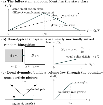
Three tests for an extensive entropy. A globally pure state has a Page-like turnover because $S_A=S_B$, while a mixed thermal state reaches the nonzero full-system entropy. Haar-typical reduced states are nearly maximally mixed, with a Page deficit controlled by the Hilbert-space ratio $m/n$. Local unitary dynamics produces the volume-law plateau only after entanglement has propagated through the region from its boundary.

State family	Global state	Small-region coefficient	Full-system endpoint	Mechanism
Haar-random vector	pure	near $\ln q$	zero	concentration in Hilbert space
Gibbs state	mixed	$s_{\mathrm{th}}(\beta)$	$s_{\mathrm{th}}V$	ensemble mixedness
chaotic eigenstate	pure	$s_{\mathrm{th}}(e)$ under ETH conditions	zero	eigenstate entanglement
thermalizing quench state	pure	late-time $s_{\mathrm{eq}}$	zero	dynamical entanglement production
integrable quench state	pure	generalized-ensemble density	zero	quasiparticle pairs and conserved occupations
localized eigenstate	pure	often zero volume coefficient	zero	quasi-local integrals of motion

The table lists leading expectations, not universal theorems. Each row needs its own limit and exceptions.

Haar-Random Pure States

The ensemble

Let

$$\mathcal H = \mathcal H_A \otimes \mathcal H_B,$$

with

$$\begin{aligned} m &:= \dim\mathcal H_A, \\ n &:= \dim\mathcal H_B, \quad m\le n. \end{aligned}$$

A Haar-random pure state is sampled uniformly from the unit sphere using the unitarily invariant measure. In a product basis,

$$\lvert\Psi\rangle = \sum_{i=1}^{m} \sum_{\mu=1}^{n} X_{i\mu} \lvert i\rangle_A \lvert\mu\rangle_B,$$

where the normalized coefficient matrix $X$ can be generated from independent complex Gaussian entries followed by normalization.

The reduced state is

$$\rho_A = XX^\dagger.$$

It is a normalized Wishart-type random matrix. When $n$ is much larger than $m$, its eigenvalues concentrate near $1/m$.

Average purity

The exact Haar average of the purity is

$$\left\langle \operatorname{Tr}\rho_A^2 \right\rangle = \frac{m+n}{mn+1}.$$

For

$$n\gg m,$$

this becomes

$$\left\langle \operatorname{Tr}\rho_A^2 \right\rangle = \frac1m + \frac1n + O \left( \frac{1}{mn} \right).$$

The maximally mixed value is $1/m$. The environment dimension controls the excess purity.

Exact Page mean

The exact mean von Neumann entropy is

$$\left\langle S_A\right\rangle = \sum_{k=n+1}^{mn} \frac1k - \frac{m-1}{2n}.$$

Using harmonic numbers,

$$\left\langle S_A\right\rangle = H_{mn} - H_n - \frac{m-1}{2n}.$$

For large $m,n$ with $m\le n$,

$$\left\langle S_A\right\rangle = \ln m - \frac{m}{2n} + O \left( \frac{1}{mn} + \frac{1}{n^2} \right).$$

The Page deficit

$$\delta_{\mathrm P} := \ln m - \left\langle S_A\right\rangle$$

is therefore approximately

$$\delta_{\mathrm P} \simeq \frac{m}{2n}.$$

At an equal bipartition,

$$m=n\to\infty,$$

the deficit approaches

$$\delta_{\mathrm P} \longrightarrow \frac12$$

nat. The entropy remains extensive; the correction is only $O(1)$.

Lattice Page curve

For $V$ unconstrained $q$-level sites and

$$f\le\frac12,$$

set

$$m=q^{fV}, \qquad n=q^{(1-f)V}.$$

Then

$$\begin{aligned} \left\langle S_A(f)\right\rangle &= fV\ln q \\ &\quad - \frac12 q^{-(1-2f)V} + \cdots. \end{aligned}$$

For fixed

$$0<f<\frac12,$$

the correction is exponentially small in $V$. At $f=1/2$, it becomes the finite Page correction $1/2$.

Complement symmetry supplies the other half:

$$\left\langle S_A(f)\right\rangle = \left\langle S_A(1-f)\right\rangle.$$

Thus the leading curve is

$$\left\langle S_A(f)\right\rangle = V\ln q\, \min(f,1-f) + O(1).$$

Typical means more than average

The Page formula is an ensemble mean. Concentration of measure shows that, in large Hilbert spaces, almost every Haar-random vector has entropy close to that mean. Atypical low-entanglement vectors occupy a very small fraction of the unit sphere.

This is why a “generic vector” is volume-law entangled. It does not imply that every physically prepared state is Haar random. Ground states, low-depth circuits, symmetry-restricted states, and finite-energy states sample highly structured subsets of Hilbert space.

Haar random is not finite-temperature random

A Haar vector in the full tensor-product Hilbert space is locally close to infinite temperature. It has no sharp energy density for a generic local Hamiltonian.

A finite-temperature typical state must instead be restricted or weighted, for example by:

• a microcanonical energy shell;
• a fixed charge sector;
• a filtered random vector;
• an energy-weighted thermal pure state;
• actual Hamiltonian eigenstates satisfying ETH.

The effective state-counting entropy of the restricted subspace replaces $V\ln q$ as the leading density.

Symmetry and charge constraints

Suppose the allowed Hilbert space is a sector

$$\mathcal H_Q \subset \mathcal H_A\otimes\mathcal H_B.$$

It generally decomposes as

$$\mathcal H_Q = \bigoplus_{q_A} \mathcal H_{A,q_A} \otimes \mathcal H_{B,Q-q_A}.$$

The reduced state is block diagonal in $q_A$. Its entropy separates into charge uncertainty and within-sector entropy:

$$S_A = H \left( \{p_{q_A}\} \right) + \sum_{q_A} p_{q_A} S \left( \rho_{A,q_A} \right).$$

The leading term can remain a volume law, while Gaussian charge fluctuations generate logarithmic corrections. Comparing an unconstrained Page curve with fixed-charge data without adjusting the reference ensemble gives a false deficit.

Mixed Thermal States

Global Gibbs entropy

For

$$\rho_\beta = \frac{e^{-\beta H}}{Z(\beta)}, \qquad Z(\beta) = \operatorname{Tr}e^{-\beta H},$$

the global entropy is

$$\begin{aligned} S(\rho_\beta) &= -\operatorname{Tr} \left( \rho_\beta\ln\rho_\beta \right) \\ &= \ln Z + \beta \langle H\rangle_\beta. \end{aligned}$$

For a regular thermodynamic phase,

$$S(\rho_\beta) = s_{\mathrm{th}}(\beta)V + o(V).$$

The coefficient is ordinary thermodynamic entropy density.

Subsystem volume law

For a regular region much larger than the thermal correlation length,

$$S(\rho_{\beta,A}) = s_{\mathrm{th}}(\beta)V_A + O \left( |\partial A| \right) + o(V_A),$$

where

$$\rho_{\beta,A} = \operatorname{Tr}_B\rho_\beta.$$

The exact reduced state is not generally

$$\frac{e^{-\beta H_A}} {\operatorname{Tr}_A e^{-\beta H_A}},$$

because crossing interactions and the environment modify its modular Hamiltonian. The bulk coefficient can agree even when the boundary operator does not.

Infinite-temperature counterexample

At

$$\beta=0,$$

an unconstrained $q$-level lattice has

$$\rho_0 = \frac{I}{q^V} = \bigotimes_{x=1}^{V} \frac{I_x}{q}.$$

For any set of $V_A$ sites,

$$\rho_{0,A} = \frac{I_A}{q^{V_A}}, \qquad S_A = V_A\ln q.$$

This is a maximal volume law. Nevertheless,

$$I(A:B)=0,$$

and the global state is a product across every site partition. The entropy is local mixedness, not entanglement.

No Page turnover

For a mixed thermal state,

$$S_A \sim s_{\mathrm{th}}fV$$

can continue through $f=1/2$ to

$$S_A(f=1) = S(\rho_\beta) \sim s_{\mathrm{th}}V.$$

There is no complement equality

$$S_A=S_B$$

unless special conditions happen to enforce it. Instead, the Araki–Lieb inequality gives

$$\left| S_A-S_B \right| \le S_{AB}.$$

Correlations live in the residual

For a short-range thermal phase, write

$$\begin{aligned} S_A &= s_{\mathrm{th}}V_A + \delta_A, \\ S_B &= s_{\mathrm{th}}V_B + \delta_B, \\ S_{AB} &= s_{\mathrm{th}}V + \delta_{AB}. \end{aligned}$$

Then

$$I(A:B) = \delta_A + \delta_B - \delta_{AB}.$$

The leading volume terms cancel. The future many-body mutual-information page owns this diagnostic; the important point here is that a subsystem volume law can coexist with weak boundary-local total correlation.

Thermal critical and long-range caveats

The expansion

$$S_A = s_{\mathrm{th}}V_A + O \left( |\partial A| \right)$$

assumes a conventional thermodynamic limit. Near thermal critical points, with long-range interactions, or in constrained and gauge systems, boundary and subleading terms can scale anomalously. The existence of a bulk entropy density can survive, but the correction should not be assumed to be a featureless area term.

Chaotic Energy Eigenstates

A pure eigenstate has no global entropy

Let

$$H\lvert E_n\rangle = E_n\lvert E_n\rangle.$$

The eigenstate density operator

$$\rho^{(n)} = \lvert E_n\rangle\langle E_n\rvert$$

is pure:

$$S \left( \rho^{(n)} \right) = 0.$$

Its subsystem state

$$\rho_A^{(n)} = \operatorname{Tr}_B \lvert E_n\rangle\langle E_n\rvert$$

can nevertheless have extensive entropy. That entropy is genuine entanglement across $A\vert B$.

From local ETH to subsystem ETH

The standard eigenstate-thermalization ansatz organizes matrix elements of a sufficiently simple observable $O$ as

$$\begin{aligned} O_{mn} &= \overline O(\bar E) \delta_{mn} \\ &\quad + e^{-S(\bar E)/2} f_O(\bar E,\omega) R_{mn}, \end{aligned}$$

where

$$\bar E = \frac{E_m+E_n}{2}, \qquad \omega = E_m-E_n.$$

The smooth diagonal part reproduces equilibrium values, while the entropy-suppressed off-diagonal part controls fluctuations and dynamics. This ansatz is a hypothesis for suitable chaotic systems and observable classes, not a theorem for every Hamiltonian.

A stronger subsystem form compares reduced density operators:

$$\rho_A^{(n)} \approx \rho_{A,\mathrm{mc}}(E_n,\Delta E),$$

where

$$\rho_{A,\mathrm{mc}} = \operatorname{Tr}_B \rho_{\mathrm{mc}}.$$

When this approximation is controlled, it implies agreement for all bounded operators supported in $A$, not merely one chosen observable.

Entropy density under ETH

For a homogeneous chaotic eigenstate at energy density

$$e_n = \frac{E_n}{V},$$

the subsystem entropy is expected to satisfy

$$S_A^{(n)} = s_{\mathrm{th}}(e_n)V_A + o(V_A)$$

for a growing region that remains smaller than its environment and after all conserved densities are matched.

The coefficient is thermodynamic because it is determined by the density of states near $e_n$. The entropy is entanglement because the global eigenstate is pure. Both statements can be true without identifying the two global density operators.

Finite subsystem fractions

There are three distinct limits:

• Strictly local subsystem: $V_A$ is fixed while $V\to\infty$.
• Subextensive thermodynamic region: $V_A\to\infty$ while $V_A/V\to0$.
• Extensive subsystem: $V_A/V\to f>0$.

Reduced-state equality is cleanest in the first regime. Entropy-density agreement can persist in the second and, for von Neumann entropy in chaotic systems, over fixed fractions below one half.

Global purity imposes

$$S_A^{(n)}(f) = S_A^{(n)}(1-f).$$

The leading finite-fraction curve is therefore Page-like:

$$S_A^{(n)}(f) \sim s_{\mathrm{th}}(e_n)V \min(f,1-f).$$

This is a leading thermodynamic form, not an exact finite-size formula. Energy conservation, charge sectors, boundaries, and eigenstate-to-eigenstate fluctuations alter the correction near $f=1/2$.

Energy-shell random states versus full Haar states

A full Haar vector samples the entire Hilbert space and has slope near

$$\ln q.$$

A finite-energy eigenstate samples a much smaller effective shell whose logarithmic dimension is

$$\ln\Omega(E,\Delta E) = s_{\mathrm{th}}(e)V + o(V).$$

Consequently,

$$s_{\mathrm{th}}(e) \le \ln q,$$

with equality only at an appropriate infinite-temperature point in the unconstrained finite-dimensional system.

The difference is essential. A highly entangled eigenstate need not be locally maximally mixed; it is locally thermal at its own energy and conserved densities.

Rényi entropies retain more global information

For

$$\alpha>0, \qquad \alpha\ne1,$$

the Rényi entropy is

$$S_\alpha(A) = \frac{1}{1-\alpha} \ln \operatorname{Tr}\rho_A^\alpha.$$

In an extensive subsystem of a chaotic finite-energy eigenstate, the Rényi entropy density can depend nonlinearly on $f$. It need not equal the Rényi entropy density of the canonical mixed state at the same mean energy, even when the von Neumann densities agree.

The reason is spectral weighting. For $\alpha>1$, large eigenvalues of $\rho_A$ receive enhanced weight. Energy sharing between $A$ and $B$ and fluctuations across the microcanonical shell then affect the saddle point.

Therefore:

$$\begin{gathered} \text{von Neumann density agreement} \\ \centernot\Longrightarrow \\ \text{full reduced-spectrum agreement}. \end{gathered}$$

ETH evidence and limits

A responsible eigenstate volume-law claim states:

• the energy-density window;
• symmetry and momentum sector;
• subsystem-fraction range;
• observable or norm used for ETH;
• finite-size extrapolation;
• whether rare eigenstates were excluded;
• whether Rényi indices beyond one were tested.

ETH can fail or require replacement in integrable, localized, fragmented, scarred, or otherwise constrained systems. The phrase “highly excited” does not establish chaos.

Post-Quench Volume Laws

Quantum Quenches defines the switch, final-energy distribution, and early-time correlation and entanglement diagnostics. This section owns the extensive subsystem-entropy scaling that can emerge later.

Global unitarity and subsystem growth

Let a pure initial state evolve as

$$\lvert\Psi(t)\rangle = e^{-iHt/\hbar} \lvert\Psi(0)\rangle.$$

The global state remains pure:

$$S_{AB}(t)=0.$$

The reduced state

$$\rho_A(t) = \operatorname{Tr}_B \lvert\Psi(t)\rangle \langle\Psi(t)\rvert$$

does not evolve unitarily on $A$ alone. Interactions transfer initially local information into correlations across the cut, allowing $S_A(t)$ to grow.

A boundary-rate constraint

For bounded finite-range interactions and finite local dimension, entanglement can be produced across a smooth cut only by terms near that cut. A schematic rate bound is

$$\left| \frac{dS_A}{dt} \right| \le C |\partial_E A|,$$

where $C$ depends on local interaction norms, range, local dimension, and units.

Starting from a low-entanglement state,

$$S_A(t) \lesssim S_A(0) + C |\partial_E A|t.$$

At fixed $t$, the contribution is boundary controlled. To build

$$S_A \sim s_{\mathrm{eq}}V_A$$

in a region of linear size $R$, local dynamics requires a time of order

$$t_{\mathrm{sat}} \sim \frac{R}{v_E}.$$

This reconciles local production with a late-time volume law.

One-dimensional ballistic form

For an interval of length $\ell$ after a homogeneous thermalizing quench, a useful leading form is

$$S_A(t) \simeq \begin{cases} 2s_{\mathrm{eq}}v_Et, & t<t_{\mathrm{sat}}, \\ s_{\mathrm{eq}}\ell, & t>t_{\mathrm{sat}}, \end{cases}$$

with

$$t_{\mathrm{sat}} \simeq \frac{\ell}{2v_E}.$$

The factor of two counts the two endpoints of a bulk interval. For a half-chain with one cut, the convention changes. Boundary conditions, initial correlations, conservation laws, and inhomogeneity modify the crossover.

The entanglement velocity $v_E$ is defined by the entropy-production slope after dividing by the equilibrium entropy density and boundary factor. It is not automatically the quasiparticle group velocity, transport velocity, butterfly velocity, or Lieb–Robinson velocity.

Integrable quasiparticle formula

In a homogeneous one-dimensional integrable quench, the initial state can emit entangled quasiparticle pairs of species $a$ and rapidity $\lambda$. In the space-time scaling limit, an interval entropy often takes the form

$$\begin{aligned} S_A(t) &= \sum_a \int d\lambda\, s_a(\lambda) \\ &\quad\times \min \left[ 2 \left| v_a(\lambda) \right| t, \ell \right]. \end{aligned}$$

Here:

• $v_a(\lambda)$ is the dressed quasiparticle velocity;
• $s_a(\lambda)$ is the contribution to the stationary thermodynamic entropy density;
• the pair structure and homogeneous initial state are part of the approximation;
• the exact integration measure and species sum are model dependent.

At early times,

$$\begin{aligned} S_A(t) &\sim 2t \sum_a \int d\lambda\, \\ &\quad \left| v_a(\lambda) \right| s_a(\lambda). \end{aligned}$$

At late times,

$$S_A(t) \sim \ell \sum_a \int d\lambda\, s_a(\lambda).$$

The plateau density is the entropy density of the appropriate stationary generalized ensemble, not necessarily a canonical Gibbs ensemble.

Chaotic growth and entanglement membranes

Random local circuits and coarse-grained chaotic dynamics support a geometric description in which entanglement is obtained from a minimal membrane or cut through space-time. In one dimension, the leading entropy grows linearly in time before saturation:

$$S_A(t) \sim s_{\mathrm{eq}}v_E |\partial A|t.$$

Fluctuations and subleading broadening can have additional universal structure in random circuits. Those details depend on the circuit ensemble and Rényi index; the leading message here is the conversion

$$\begin{gathered} \text{boundary production rate} \\ \Downarrow \\ \text{volume-law plateau}. \end{gathered}$$

Which velocity?

Several velocities can coexist:

Velocity	Operational meaning
$v_{\mathrm{LR}}$	upper locality-cone scale from a Lieb–Robinson bound
$v_B$	spreading speed of an operator or out-of-time-order front
$v_E$	coarse-grained entanglement-production speed
$v_{\mathrm{tr}}$	transport speed or scale for a conserved density
$v_a(\lambda)$	quasiparticle group or dressed velocity

They need not be equal. Entanglement can spread ballistically while energy transport is diffusive. In integrable systems, a distribution of quasiparticle velocities replaces one universal front speed.

Saturation ensemble

The late-time coefficient depends on the information retained by the dynamics:

Dynamics	Candidate plateau density
generic energy-conserving chaos	thermal or microcanonical $s_{\mathrm{th}}(e)$
integrable Hamiltonian	generalized-ensemble or Yang–Yang entropy density
generic Floquet system without conservation	often infinite-temperature density
many-body localized system	nonthermal, initial-state-dependent density
fragmented dynamics	entropy density within the accessible Krylov sector

Matching a plateau to one ensemble requires matching every exact conserved quantity and the accessible Hilbert-space sector.

Finite size and recurrences

In a finite closed system, late-time entropy fluctuates around its plateau. Exact or approximate recurrences can occur on much longer timescales. The useful volume-law statement concerns a time window:

$$t_{\mathrm{local}} \ll t \ll t_{\mathrm{rec}},$$

after local equilibration and before recurrence physics dominates.

Time averaging can suppress fluctuations, but

$$S \left( \overline{\rho_A} \right)$$

is not generally equal to

$$\overline{ S \left( \rho_A(t) \right) }.$$

Entropy is nonlinear, so the averaging protocol must be declared.

Compression and Circuit Depth

Exponential Schmidt-rank demand

Across a cut, any exact representation with Schmidt rank $\chi$ satisfies

$$S_A \le \ln\chi.$$

A volume law

$$S_A = s_{\mathrm{vol}}V_A + o(V_A)$$

therefore requires

$$\chi \ge \exp \left[ s_{\mathrm{vol}}V_A + o(V_A) \right].$$

For a central cut of a chain, this is exponential in system size. It explains the rapid growth of resources in exact matrix-product-state time evolution after a global quench.

Time-dependent bond dimension

If the cut entropy grows as

$$S(t) \simeq s_{\mathrm{eq}}v_Et,$$

then exact Schmidt capacity requires

$$\chi(t) \gtrsim \exp \left( s_{\mathrm{eq}}v_Et \right).$$

Even before finite-size saturation, the required bond dimension grows exponentially in time.

Truncation may extend the reachable window for local observables, but then the discarded Schmidt tail, energy drift, conservation laws, and observable-specific error must be monitored. A small energy error does not certify the full state.

Local circuit depth

A depth-$d$ circuit of bounded-range gates acting on a product state can entangle a spatial region only through gates within distance $O(d)$ of its boundary. Its entropy obeys a schematic bound

$$S_A \le C d |\partial_E A|.$$

For a regular region of linear size $R$,

$$\frac{V_A}{|\partial_E A|} \sim R.$$

Producing a full spatial volume law therefore requires

$$d = \Omega(R)$$

with local gates. A Haar-random vector may be typical in Hilbert space while requiring a deep local circuit to prepare.

Entropy is not the whole complexity

Volume-law entanglement obstructs low-bond-dimension descriptions, but it does not uniquely determine:

• circuit complexity;
• sign or phase structure;
• stabilizer or Gaussian simulability;
• sampling complexity;
• local-observable complexity;
• compressibility in a nonspatial partition.

For example, some stabilizer states have extensive bipartite entropy yet remain efficiently describable in a stabilizer formalism. The simulation claim must name the representation and task.

Exceptions and Nonthermal Volume Laws

Integrable eigenstates and quenches

Integrable systems have extensive conserved quantities. Typical eigenstates within a macrostate can still have volume-law entanglement, but the coefficient and reduced-state structure are controlled by the conserved occupations rather than ordinary ETH.

After a quench, local observables may relax to a generalized Gibbs ensemble. The late-time entropy density can agree with an appropriate Yang–Yang entropy while differing from the canonical thermal entropy at the same mean energy.

Thus:

$$\begin{gathered} \text{volume law} \\ \centernot\Longrightarrow \\ \text{eigenstate thermalization}. \end{gathered}$$

Many-body localization

In an idealized fully many-body localized regime:

• individual finite-energy-density eigenstates can obey an area law;
• a low-entanglement initial state can show logarithmic entanglement growth;
• the long-time entropy can become extensive with a subthermal, initial-state-dependent coefficient;
• local observables retain memory of initial conditions.

The combination

$$S_A(t) \sim \ln t$$

before a nonthermal extensive plateau is qualitatively different from ballistic thermalizing growth. Finite-size drifts and rare-region effects make localization claims especially sensitive to system size and time window.

Scars and fragmented Hilbert spaces

Quantum many-body scars are atypical eigenstates with anomalous dynamics or low entanglement embedded in spectra whose typical states may be volume law. Hilbert-space fragmentation splits dynamics into disconnected sectors, so a state explores only one component.

The correct reference dimension is then

$$\dim\mathcal K_{\mathrm{accessible}},$$

not the full Hilbert-space dimension. An apparently submaximal volume-law coefficient may reflect a small accessible sector rather than weak entanglement inside that sector.

Floquet systems

A generic periodically driven interacting system without conserved energy can heat toward an infinite-temperature-like state within its symmetry sector. Floquet eigenstates and late-time states may then approach the maximal volume-law density.

Exceptions include:

• Floquet many-body localization;
• prethermal regimes at high drive frequency;
• exact conservation laws;
• kinetic constraints;
• scarred subspaces.

The observation of a volume law does not by itself establish indefinite heating.

Monitored and open dynamics

Measurements and environmental coupling can compete with unitary entanglement production. Monitored circuits can exhibit transitions between volume-law and area-law trajectory entanglement. An ensemble-averaged density operator can meanwhile become highly mixed for a different reason.

Trajectory entropy, averaged trajectory entropy, and entropy of the averaged state are distinct:

$$\overline{ S \left( \rho_A^{\mathrm{traj}} \right) } \ne S \left( \overline{ \rho_A^{\mathrm{traj}} } \right)$$

in general.

This page focuses on closed-system volume laws; open and monitored settings require their own measurement protocol.

Long-range and nonlocal couplings

For power-law or all-to-all interactions, the boundary-rate picture can fail or change. Entanglement may be generated throughout a region without waiting a time proportional to its linear size.

The volume-law definition survives, but statements about $v_E$, causal cones, and depth lower bounds must be adapted to the actual interaction graph.

A designed pure volume-law state need not be chaotic

Pair each of $N$ qudits in $A$ with one qudit in $B$:

$$\lvert\Psi\rangle = \bigotimes_{j=1}^{N} \frac1{\sqrt q} \sum_{a=0}^{q-1} \lvert a\rangle_{A_j} \lvert a\rangle_{B_j}.$$

Then

$$\rho_A = \frac{I_A}{q^N}, \qquad S_A = N\ln q.$$

This is a maximal pure-state volume law across the chosen partition, constructed from independent pairs. It has neither Haar randomness nor ETH. If the partners are spatially far apart, it also requires long-range preparation or depth growing with their separation.

Reliable Numerical Diagnosis

Step 1: write the state ledger

Record the actual object:

$$\begin{gathered} \rho_\beta, \qquad \rho_{\mathrm{mc}}, \qquad \lvert E_n\rangle\langle E_n\rvert, \\ \lvert\Psi(t)\rangle\langle\Psi(t)\rvert, \qquad \rho_{\mathrm{traj}}, \qquad \overline\rho. \end{gathered}$$

Then state whether the reported entropy is global, reduced, time averaged, disorder averaged, or trajectory averaged.

Step 2: vary both region and total size

For each total size $V$, compute several fractions

$$f = \frac{V_A}{V}.$$

Inspect:

$$\frac{S_A}{V_A}$$

for the small-region density and

$$\frac{S_A}{V}$$

for the finite-fraction shape.

A pure Page-like curve should satisfy:

$$S_A(f) = S_A(1-f), \qquad S_A(1)=0.$$

A mixed thermal curve should approach the nonzero global entropy at $f=1$.

Step 3: fit competing corrections

Compare models such as

$$S_A = sV_A + a|\partial A| + b\ln V_A + c$$

over the same size window. Remove the smallest sizes and test coefficient stability. On a chain, include open-boundary and parity oscillations when present.

Report the slope uncertainty together with the assumed correction. A linear fit with an unstable intercept is not an asymptotic diagnosis.

Step 4: match the sector

Resolve exact symmetries before comparing with random-state or thermal predictions. Within a fixed charge $Q$, use:

$$\rho_{\mathrm{ref}} = \frac{P_Q}{\operatorname{Tr}P_Q}$$

at infinite temperature, not $I/q^V$ on the full space.

For eigenstates, compare states within one symmetry sector and a narrow energy-density window. Mixing sectors can create spurious degeneracies, entropy offsets, and apparent ETH violations.

Step 5: check more than von Neumann entropy

Useful companion diagnostics include:

• Rényi entropies;
• the entanglement spectrum;
• subsystem energy and charge distributions;
• mutual information;
• local observable agreement with an ensemble;
• trace distance for sufficiently small subsystems;
• energy variance and conserved-charge drift;
• transfer-matrix correlation length in tensor-network data.

Equal entropy values do not imply equal reduced states.

Step 6: audit bond-dimension saturation

For an MPS,

$$S_A \le \ln\chi$$

across one cut. If a purported physical plateau tracks $\ln\chi$ as $\chi$ changes, it is a numerical ceiling.

During time evolution, record:

• maximum bond dimension;
• discarded weight at every step;
• accumulated norm and energy errors;
• entropy at several cuts;
• convergence of local observables;
• the time at which different $\chi$ curves separate.

The last converged time can be much earlier for entanglement-sensitive observables than for one-site expectation values.

Step 7: extract a growth velocity carefully

In one dimension, fit the early-time window to

$$S_A(t) = r_Et+c$$

only after microscopic transients and before finite-size saturation. For a bulk interval with two endpoints,

$$v_E = \frac{r_E}{2s_{\mathrm{eq}}}.$$

The equilibrium density must be measured independently. If $s_{\mathrm{eq}}$ is replaced by $\ln q$ in a finite-energy quench, the inferred velocity is biased.

Repeat over several interval lengths. A genuine ballistic regime has a length-independent slope and saturation time proportional to $\ell$ over a controlled window.

Common Mistakes

• Calling an extensive mixed-state entropy entanglement. At infinite temperature, $S_A=V_A\ln q$ can coexist with zero mutual information.
• Extrapolating a pure-state line past half the system. Complement symmetry forces a turnover.
• Treating the Page curve as a dynamical theorem. Haar typicality does not specify preparation depth or Hamiltonian evolution.
• Comparing finite-energy eigenstates with full-Hilbert-space Haar vectors. The energy shell has a smaller entropy density.
• Applying ETH by vocabulary. Nonintegrability, sector resolution, energy window, and finite-size evidence must be shown.
• Assuming every highly excited eigenstate is thermal. Integrable, localized, fragmented, and scarred exceptions exist.
• Equating von Neumann and Rényi thermalization. Extensive-subsystem Rényi densities can retain finite-fraction dependence.
• Calling every late-time plateau canonical. Generalized ensembles, Floquet heating, localization, and constraints produce different coefficients.
• Identifying $v_E$ with every other velocity. Information, transport, quasiparticle, and locality speeds are operationally distinct.
• Ignoring the order of limits. Fixed time followed by $R\to\infty$ probes boundary growth; $t\sim R$ can reveal a volume-law plateau.
• Mistaking finite-$\chi$ saturation for physics. A matrix-product ansatz imposes $S\le\ln\chi$.
• Inferring full complexity from entropy alone. Representation, observable, and simulation task still matter.
• Dropping symmetry-sector corrections. Fixed charges alter both the leading reference density and logarithmic terms.
• Averaging before versus after taking entropy. Entropy is nonlinear.

Exercises

1. The Page curve of a qudit chain

Consider a chain of $V$ qudits with local Hilbert-space dimension $q$. A Haar-random pure state is drawn from the full Hilbert space. Let $A$ contain the fraction $f$ of the sites, with $0<f\leq 1/2$.

1. Identify the subsystem dimensions $m$ and $n$.
2. Use the Page formula to find the leading entropy and its first correction.
3. Compare the correction at fixed $f<1/2$ with the correction at $f=1/2$.
4. Extend the answer to $f>1/2$.

Solution

For $V_A=fV$ and $V_{\bar A}=(1-f)V$,

$$m=q^{fV}, \qquad n=q^{(1-f)V}.$$

Because $f\leq 1/2$, one has $m\leq n$. The large-dimension Page formula gives

$$\mathbb E_{\mathrm{Haar}}S_A = \ln m - \frac{m}{2n} + O\!\left(\frac{1}{n^2}\right).$$

Substitution yields

$$\begin{aligned} \mathbb E_{\mathrm{Haar}}S_A &= fV\ln q - \frac{1}{2} q^{-(1-2f)V} \\ &\quad + O\!\left(q^{-2(1-f)V}\right). \end{aligned}$$

At any fixed $f<1/2$, the deficit from maximal entropy is exponentially small in $V$. At the symmetric cut,

$$\begin{aligned} f &= \frac12, \\ \mathbb E_{\mathrm{Haar}}S_A &= \frac{V}{2}\ln q - \frac12 + o(1). \end{aligned}$$

so the deficit approaches one-half nat rather than zero.

For $f>1/2$, global purity gives $S_A=S_{\bar A}$. Therefore,

$$\begin{aligned} \mathbb E_{\mathrm{Haar}}S_A &= V\ln q\, \min(f,1-f) \\ &\quad + O(1). \end{aligned}$$

The resulting tent-shaped finite-fraction curve is the Page curve of a pure random state.

2. Purity as a quick typicality bound

Let a Haar-random pure state live in $\mathbb C^m\otimes\mathbb C^n$ with $m=4$ and $n=64$.

1. Compute the mean subsystem purity.
2. Compare it with the minimum possible purity.
3. Use $S(\rho)\geq-\ln\operatorname{Tr}\rho^2$ and Jensen’s inequality to obtain a lower bound on the mean von Neumann entropy.

Solution

Lubkin’s exact average purity is

$$\mathbb E_{\mathrm{Haar}} \operatorname{Tr}\rho_A^2 = \frac{m+n}{mn+1}.$$

For $m=4$ and $n=64$,

$$\mathbb E_{\mathrm{Haar}} \operatorname{Tr}\rho_A^2 = \frac{68}{257} \approx 0.2646.$$

The maximally mixed state on $\mathbb C^4$ has purity $1/m=1/4=0.25$, so the random subsystem is already close to maximally mixed.

For every density operator,

$$S(\rho_A) \geq -\ln\operatorname{Tr}\rho_A^2.$$

Because $-\ln x$ is convex, Jensen’s inequality gives

$$\begin{aligned} \mathbb E_{\mathrm{Haar}}S_A &\geq \mathbb E_{\mathrm{Haar}} \left[ -\ln\operatorname{Tr}\rho_A^2 \right] \\ &\geq -\ln \mathbb E_{\mathrm{Haar}} \operatorname{Tr}\rho_A^2 \\ &= -\ln\!\left(\frac{68}{257}\right) \approx 1.329. \end{aligned}$$

The maximum is $\ln4\approx1.386$. Purity therefore supplies a short, quantitative certificate of near-maximal typical entanglement, although it does not determine the full entanglement spectrum.

3. An endpoint test for pure and mixed volume laws

Two candidate finite-fraction entropy curves are

$$\begin{aligned} g_1(f) &= sV\min(f,1-f), \\ g_2(f) &= sVf. \end{aligned}$$

Evaluate both at $f=1/4$, $1/2$, $3/4$, and $1$. Which curve can describe a globally pure state? Why can small-subsystem data alone fail to distinguish them?

Solution

The values are:

$f$	$g_1(f)/(sV)$	$g_2(f)/(sV)$
$1/4$	$1/4$	$1/4$
$1/2$	$1/2$	$1/2$
$3/4$	$1/4$	$3/4$
$1$	$0$	$1$

A globally pure state must obey

$$S_A = S_{\bar A}, \qquad S_{\mathrm{all}} = 0.$$

Thus $g_1$ has the required complement symmetry and endpoint. The curve $g_2$ instead has nonzero entropy $sV$ for the whole system and is compatible with a mixed thermodynamic state.

For $f\leq1/2$, the two expressions coincide. A fit using only small subsystems can therefore recover the same extensive coefficient from two states with completely different global purity. Finite-fraction data or an independent purity test is required.

4. A maximal volume law without entanglement

On $V$ qudits, consider the infinite-temperature state

$$\rho_\infty = \frac{I}{q^V}.$$

For a bipartition into $A$ and $B$, compute $S_A$, $S_B$, $S_{AB}$, and $I(A:B)$. Is this state entangled?

Solution

The state factorizes:

$$\rho_\infty = \left(\frac{I_A}{q^{V_A}}\right) \otimes \left(\frac{I_B}{q^{V_B}}\right).$$

Its entropies are

$$S_A = V_A\ln q, \qquad S_B = V_B\ln q,$$

and

$$S_{AB} = V\ln q.$$

Consequently,

$$\begin{aligned} I(A:B) &= S_A+S_B-S_{AB} \\ &= 0. \end{aligned}$$

The state is a product of local maximally mixed states and is therefore separable. Its maximal volume-law subsystem entropy is entirely thermodynamic uncertainty, not entanglement. This example is the cleanest warning against using the phrase “volume-law entanglement” for an arbitrary mixed state.

5. Fixed filling changes the random-state coefficient

Consider $V$ spin-$1/2$ sites restricted to the sector with exactly $N=\nu V$ up spins, where $0<\nu<1$ and $\nu V$ is an integer.

1. Estimate the sector dimension for large $V$.
2. Find its entropy density.
3. Compare it with the full-Hilbert-space value $\ln2$.

Solution

The fixed-filling sector has dimension

$$D_{V,N} = \binom{V}{N} = \binom{V}{\nu V}.$$

Stirling’s approximation gives

$$\binom{V}{\nu V} \sim \frac{ \exp\!\left[Vh_2(\nu)\right] }{ \sqrt{2\pi V\nu(1-\nu)} },$$

where

$$h_2(\nu) = -\nu\ln\nu - (1-\nu)\ln(1-\nu)$$

is the binary entropy. Hence

$$\ln D_{V,N} = Vh_2(\nu) - \frac12\ln V + O(1).$$

The sector entropy density is $h_2(\nu)$. It satisfies

$$h_2(\nu) \leq \ln2,$$

with equality only at half filling, $\nu=1/2$. Random-state benchmarks must therefore be drawn in the same symmetry sector as the physical state. Using a full-Hilbert-space Page slope away from half filling overestimates the available entropy density.

6. Full Haar randomness versus a finite-energy eigenstate

A local $q$-state Hamiltonian has a chaotic eigenstate at energy density $e$. Assume subsystem ETH applies and that the thermodynamic entropy density satisfies $s_{\mathrm{th}}(e)<\ln q$.

Compare the small-subsystem entropy slope, global entropy, and finite-fraction endpoint of this eigenstate with those of a Haar-random state on the full Hilbert space.

Solution

For a full-Hilbert-space Haar state and a subsystem smaller than half the system,

$$S_A \simeq V_A\ln q.$$

For the chaotic finite-energy eigenstate, subsystem ETH instead gives

$$S_A \simeq s_{\mathrm{th}}(e)V_A + o(V_A),$$

so its slope is smaller than $\ln q$ unless the energy density corresponds to infinite temperature.

Both states are globally pure:

$$S_{\mathrm{all}} = 0.$$

Both must turn over under $A\leftrightarrow\bar A$ and approach zero as $f\to1$. At leading order their finite-fraction curves have the Page-like forms

$$S_A^{\mathrm{Haar}} \sim V\ln q\,\min(f,1-f)$$

and

$$S_A^{\mathrm{eig}} \sim Vs_{\mathrm{th}}(e)\min(f,1-f),$$

subject to finite-fraction, conserved-charge, and Rényi-dependent corrections. Purity fixes the endpoint structure; the accessible energy shell fixes the thermodynamic coefficient.

7. Quench saturation and matrix-product bond dimension

Suppose the entropy of a one-dimensional interval of length $\ell$ after a homogeneous global quench is modeled by

$$S_A(t) = \min \left[ 2s_{\mathrm{eq}}v_Et,\, s_{\mathrm{eq}}\ell \right].$$

Take $\ell=100$, $v_E=0.8$, and $s_{\mathrm{eq}}=0.6$ in units where the lattice spacing and time unit are one.

1. Find the saturation time.
2. Find the plateau entropy.
3. Estimate the minimum exact MPS bond dimension needed at the plateau.

Solution

Saturation occurs when the two arguments of the minimum agree:

$$2s_{\mathrm{eq}}v_Et_{\mathrm{sat}} = s_{\mathrm{eq}}\ell.$$

The entropy density cancels, giving

$$t_{\mathrm{sat}} = \frac{\ell}{2v_E} = \frac{100}{1.6} = 62.5.$$

The plateau is

$$S_A^{\mathrm{sat}} = s_{\mathrm{eq}}\ell = 60.$$

Across a single MPS cut,

$$S_A \leq \ln\chi.$$

An exact representation therefore requires at least

$$\chi \geq e^{60} \approx 1.14\times10^{26}.$$

This enormous lower bound explains why local observables may remain numerically converged long after direct entanglement-sensitive simulation has become impractical.

8. Diagnose atypical volume-law data

For each observation below, state the first interpretation you would test and one additional diagnostic that could distinguish it from ordinary thermalizing dynamics.

1. Highly excited eigenstates obey an area law.
2. Entanglement grows approximately as $\ln t$ after a quench and later reaches a subthermal volume law.
3. A small set of finite-energy eigenstates has much lower entropy than neighboring eigenstates.
4. A periodically driven system approaches the maximal entropy density $\ln q$ within each symmetry sector.

Solution

1. Excited-state area law: test many-body localization, Hilbert-space fragmentation, or an integrable fine-tuned structure. Useful diagnostics include level statistics, transport, local integrals of motion, and stability to generic local perturbations.

2. Logarithmic growth with a subthermal plateau: test an interacting many-body-localized regime. Check memory of local initial conditions, vanishing transport, disorder-size scaling, and whether the logarithmic window survives increasing system size and bond dimension.

3. Sparse low-entanglement eigenstates: test quantum many-body scars or another weak-ergodicity-breaking mechanism. Examine their overlap with simple product states, atypical local observables, dynamical revivals, and whether the fraction of atypical states vanishes with size.

4. Maximal sector-resolved entropy under driving: test Floquet heating toward infinite temperature. Verify that local observables approach the identity ensemble within the correct symmetry sector, while excluding prethermal plateaus by varying the drive frequency and observation time.

None of these signatures is conclusive alone. Entanglement scaling should be combined with spectral, transport, observable, and finite-size evidence.

Summary

A volume law means that subsystem entropy has a nonzero density:

$$\frac{S_A}{V_A} \longrightarrow s_{\mathrm{vol}} > 0$$

in a stated thermodynamic limit. The coefficient and the finite-fraction curve depend on the state class.

For a Haar-random pure state with $m\leq n$, Page’s result gives

$$\mathbb E_{\mathrm{Haar}}S_A = \ln m - \frac{m}{2n} + \cdots.$$

At fixed subsystem fraction, global purity imposes a turnover:

$$S_A \sim sV\min(f,1-f).$$

A mixed thermal state instead has

$$S_A \sim s_{\mathrm{th}}Vf$$

and can retain a nonzero global entropy. Chaotic finite-energy eigenstates reproduce thermodynamic entropy densities for sufficiently small subsystems, but purity, conservation laws, finite-fraction effects, and the Rényi index remain essential.

After a global quench, local dynamics can generate entanglement ballistically before a volume-law plateau forms. The growth rate is constrained by locality and boundary geometry, whereas the late-time entropy is extensive. Integrable, localized, fragmented, scarred, constrained, and driven systems supply controlled exceptions to the simplest thermalizing picture.

The phrase “volume law” is therefore only the start of a diagnosis. A trustworthy claim states the entropy, state ensemble, symmetry sector, subsystem limit, global purity, finite-size corrections, and numerical convergence tests.

References

1. E. Lubkin, “Entropy of an $n$-system from its correlation with a $k$-reservoir,” Journal of Mathematical Physics 19, 1028–1031 (1978). doi:10.1063/1.523763
2. J. M. Deutsch, “Quantum statistical mechanics in a closed system,” Physical Review A 43, 2046–2049 (1991). doi:10.1103/PhysRevA.43.2046
3. D. N. Page, “Average entropy of a subsystem,” Physical Review Letters 71, 1291–1294 (1993). doi:10.1103/PhysRevLett.71.1291
4. S. K. Foong and S. Kanno, “Proof of Page’s conjecture on the average entropy of a subsystem,” Physical Review Letters 72, 1148–1151 (1994). doi:10.1103/PhysRevLett.72.1148
5. M. Srednicki, “Chaos and quantum thermalization,” Physical Review E 50, 888–901 (1994). doi:10.1103/PhysRevE.50.888
6. S. Sen, “Average entropy of a quantum subsystem,” Physical Review Letters 77, 1–3 (1996). doi:10.1103/PhysRevLett.77.1
7. H. Tasaki, “From quantum dynamics to the canonical distribution: General picture and a rigorous example,” Physical Review Letters 80, 1373–1376 (1998). doi:10.1103/PhysRevLett.80.1373
8. P. Calabrese and J. Cardy, “Evolution of entanglement entropy in one-dimensional systems,” Journal of Statistical Mechanics: Theory and Experiment 2005, P04010 (2005). doi:10.1088/1742-5468/2005/04/P04010
9. P. Hayden, D. W. Leung, and A. Winter, “Aspects of generic entanglement,” Communications in Mathematical Physics 265, 95–117 (2006). doi:10.1007/s00220-006-1535-6
10. S. Goldstein, J. L. Lebowitz, R. Tumulka, and N. Zanghì, “Canonical typicality,” Physical Review Letters 96, 050403 (2006). doi:10.1103/PhysRevLett.96.050403
11. S. Popescu, A. J. Short, and A. Winter, “Entanglement and the foundations of statistical mechanics,” Nature Physics 2, 754–758 (2006). doi:10.1038/nphys444
12. M. Rigol, V. Dunjko, and M. Olshanii, “Thermalization and its mechanism for generic isolated quantum systems,” Nature 452, 854–858 (2008). doi:10.1038/nature06838
13. J. M. Deutsch, “Thermodynamic entropy of a many-body energy eigenstate,” New Journal of Physics 12, 075021 (2010). doi:10.1088/1367-2630/12/7/075021
14. J. H. Bardarson, F. Pollmann, and J. E. Moore, “Unbounded growth of entanglement in models of many-body localization,” Physical Review Letters 109, 017202 (2012). doi:10.1103/PhysRevLett.109.017202
15. H. Kim and D. A. Huse, “Ballistic spreading of entanglement in a diffusive nonintegrable system,” Physical Review Letters 111, 127205 (2013). doi:10.1103/PhysRevLett.111.127205
16. M. Serbyn, Z. Papić, and D. A. Abanin, “Universal slow growth of entanglement in interacting strongly disordered systems,” Physical Review Letters 110, 260601 (2013). doi:10.1103/PhysRevLett.110.260601
17. L. D’Alessio, Y. Kafri, A. Polkovnikov, and M. Rigol, “From quantum chaos and eigenstate thermalization to statistical mechanics and thermodynamics,” Advances in Physics 65, 239–362 (2016). doi:10.1080/00018732.2016.1198134
18. A. M. Kaufman et al., “Quantum thermalization through entanglement in an isolated many-body system,” Science 353, 794–800 (2016). doi:10.1126/science.aaf6725
19. A. Nahum, J. Ruhman, S. Vijay, and J. Haah, “Quantum entanglement growth under random unitary dynamics,” Physical Review X 7, 031016 (2017). doi:10.1103/PhysRevX.7.031016
20. V. Alba and P. Calabrese, “Entanglement and thermodynamics after a quantum quench in integrable systems,” Proceedings of the National Academy of Sciences 114, 7947–7951 (2017). doi:10.1073/pnas.1703516114
21. A. Dymarsky, N. Lashkari, and H. Liu, “Subsystem eigenstate thermalization hypothesis,” Physical Review E 97, 012140 (2018). doi:10.1103/PhysRevE.97.012140
22. J. R. Garrison and T. Grover, “Does a single eigenstate encode the full Hamiltonian?,” Physical Review X 8, 021026 (2018). doi:10.1103/PhysRevX.8.021026
23. V. Alba and P. Calabrese, “Entanglement dynamics after quantum quenches in generic integrable systems,” SciPost Physics 4, 017 (2018). doi:10.21468/SciPostPhys.4.3.017
24. T.-C. Lu and T. Grover, “Renyi entropy of chaotic eigenstates,” Physical Review E 99, 032111 (2019). doi:10.1103/PhysRevE.99.032111
25. T. Zhou and A. Nahum, “Emergent statistical mechanics of entanglement in random unitary circuits,” Physical Review B 99, 174205 (2019). doi:10.1103/PhysRevB.99.174205
26. C. Murthy and M. Srednicki, “Structure of chaotic eigenstates and their entanglement entropy,” Physical Review E 100, 022131 (2019). doi:10.1103/PhysRevE.100.022131

Cross-Links

• Many-Body Entanglement Overview
• Entanglement Entropy in Many-Body Systems
• Thermal Entropy vs Entanglement Entropy
• Area Laws
• Entanglement Spectrum — probability distributions and level structure underlying extensive entropy.
• Mutual Information in Many-Body Systems — why extensive marginal entropies need not imply extensive shared correlation.
• Entropy in Quantum Statistical Mechanics
• Thermal Density Operators
• Microcanonical Ensemble
• Canonical Ensemble
• Ensemble Equivalence
• Thermodynamic Limit
• Variational Many-Body States
• Connected Correlation Functions
• Schmidt Decomposition
• Rényi Entropies
• Mutual Information
• Entanglement in Many-Body Physics