Entropy in Quantum Statistical Mechanics

The von Neumann formula

$$S(\rho) = -k_{\mathrm B} \operatorname{Tr} \left( \rho\ln\rho \right)$$

appears in quantum information, equilibrium statistical mechanics, entanglement theory, and nonequilibrium thermodynamics. The formula is the same, but its physical interpretation is not fixed by the formula alone. One must identify the state, the system boundary, the subsystem partition, the constraints, and any information that has been discarded.

For an equilibrium Gibbs state, $S(\rho)$ is thermodynamic entropy. For the reduced state of part of a globally pure system, it is entanglement entropy. For a generic mixed subsystem, it measures local mixedness and can contain thermal uncertainty, classical correlation, entanglement, and environmental noise. For a deliberately coarse-grained state, it depends on which distinctions were erased.

This page is the canonical home for those statistical-mechanics identifications and caveats. Entropy Overview owns the first density-operator definition, Many-Body Entanglement Overview owns the partition, state-class, measure, and scaling decision map, and Entanglement Entropy in Many-Body Systems owns spatial scaling laws and many-body computation.

Dimensionless and Thermodynamic Conventions

It is useful to separate the dimensionless state entropy

$$\mathsf S(\rho) = - \operatorname{Tr} \left( \rho\ln\rho \right)$$

from the physical entropy

$$S(\rho) = k_{\mathrm B}\mathsf S(\rho).$$

With the natural logarithm, $\mathsf S$ is measured in nats. With $\log_2$, it is measured in bits. Multiplication by $k_{\mathrm B}$ converts the dimensionless information measure into thermodynamic entropy units.

If

$$\rho = \sum_j p_j |j\rangle\langle j|$$

is the spectral decomposition, then

$$\mathsf S(\rho) = - \sum_j p_j\ln p_j.$$

Thus the von Neumann entropy is the Shannon entropy of the eigenvalue distribution. It is basis independent:

$$\mathsf S(U\rho U^\dagger) = \mathsf S(\rho).$$

The entropy is a nonlinear functional of the state, not the expectation value of a fixed observable. There is no state-independent Hermitian operator $\hat S$ satisfying $S(\rho)=\operatorname{Tr}(\rho\hat S)$ for all $\rho$.

The Context Determines the Meaning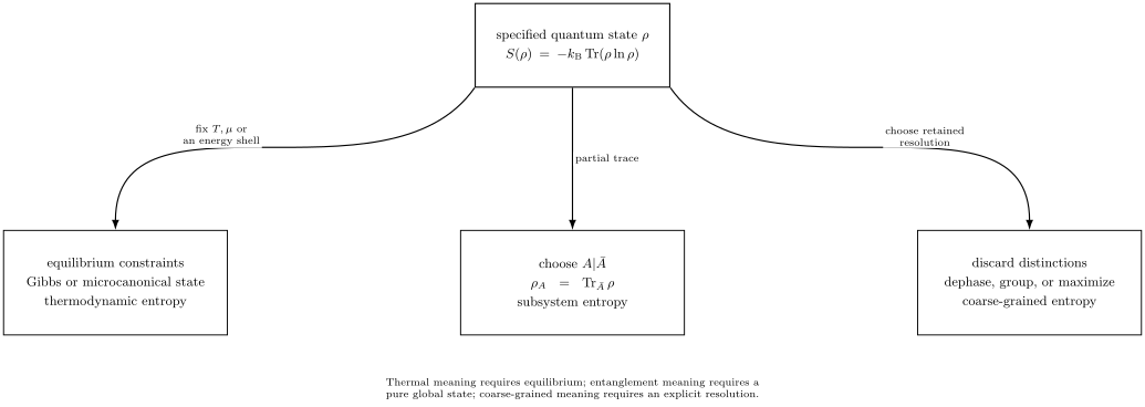

The same von Neumann functional supports several physical uses. Equilibrium constraints, a subsystem trace, and a coarse-graining operation answer different questions and generally produce different states.

Before interpreting an entropy, ask:

1. What is the state? Is it a full density operator, a reduced state, an equilibrium ensemble, or an effective state inferred from incomplete data?
2. What is the system boundary? Does $\rho$ describe the complete closed system or only a subsystem?
3. What constraints define equilibrium? Are energy, particle number, volume, or other charges fixed exactly or only in expectation?
4. What distinctions are unresolved? Has one traced out an environment, dephased phases, grouped microstates into macrostates, or maximized over unknown details?
5. What limit is being used? Is the claim finite-dimensional, thermodynamic, continuum, or asymptotic?

Two calculations can produce the same numerical entropy while answering different physical questions.

When State Entropy Is Thermodynamic Entropy

The identification

$$S_{\mathrm{th}} = S(\rho_{\mathrm{eq}})$$

is justified when $\rho_{\mathrm{eq}}$ is the equilibrium state associated with the macroscopic constraints and when the resulting entropy obeys the thermodynamic relations appropriate to those controls.

For a regular equilibrium family, this includes relations such as

$$\frac{1}{T} = \left( \frac{\partial S}{\partial U} \right)_{V,N},$$ $$S = - \left( \frac{\partial F}{\partial T} \right)_{V,N},$$

and

$$S = - \left( \frac{\partial\Omega_{\mathrm G}} {\partial T} \right)_{V,\mu}.$$

The last two derivative formulas assume the microscopic Hamiltonian has no unaccounted explicit temperature dependence. Thermodynamic Potentials owns the natural-variable and Legendre-transform framework.

The equality between state entropy and thermodynamic entropy is not a claim that every density operator is an equilibrium macrostate. A qubit prepared by a noisy device has a von Neumann entropy, but no temperature, pressure, or entropy density follows without further physical structure.

Canonical Thermal Entropy

For fixed particle number,

$$\rho_{N,\beta} = \frac{ e^{-\beta\hat H_N} }{ Z_N }, \qquad Z_N = \operatorname{Tr}_{\mathcal H_N} e^{-\beta\hat H_N}.$$

Because

$$\ln\rho_{N,\beta} = -\beta\hat H_N - \ln Z_N,$$

the entropy is

$$S_{\mathrm c} = k_{\mathrm B} \left( \ln Z_N+ \beta U \right),$$

where

$$U = \operatorname{Tr} \left( \rho_{N,\beta}\hat H_N \right).$$

Using

$$F = -k_{\mathrm B}T \ln Z_N$$

gives

$$S_{\mathrm c} = \frac{U-F}{T}.$$

For a temperature-independent Hamiltonian,

$$S_{\mathrm c} = - \left( \frac{\partial F}{\partial T} \right)_{V,N}.$$

The heat capacity satisfies

$$C_{V,N} = T \left( \frac{\partial S}{\partial T} \right)_{V,N} = k_{\mathrm B} \beta^2 \operatorname{Var}(\hat H_N).$$

The Canonical Ensemble owns the reservoir derivation and energy-fluctuation identities.

Grand-Canonical Thermal Entropy

When energy and a conserved particle number can be exchanged,

$$\rho_{\beta,\mu} = \frac{ e^{-\beta(\hat H-\mu\hat N)} }{ \Xi },$$

with

$$\Xi = \operatorname{Tr}_{\mathcal F} e^{-\beta(\hat H-\mu\hat N)}.$$

The entropy becomes

$$S_{\mathrm{gc}} = k_{\mathrm B} \left[ \ln\Xi + \beta \left( U-\mu\overline N \right) \right].$$

Since

$$\Omega_{\mathrm G} = -k_{\mathrm B}T \ln\Xi,$$

one has

$$S_{\mathrm{gc}} = \frac{ U-\mu\overline N- \Omega_{\mathrm G} }{T}.$$

At fixed $V$ and $\mu$,

$$S_{\mathrm{gc}} = - \left( \frac{\partial\Omega_{\mathrm G}} {\partial T} \right)_{V,\mu}.$$

The entropy includes uncertainty across particle-number sectors as well as within each sector. The Grand-Canonical Ensemble owns the sector decomposition and number fluctuations.

Microcanonical Entropy

Let $P_{E,\Delta}$ project onto an energy shell and let

$$W(E,\Delta) = \operatorname{Tr} P_{E,\Delta}$$

be its dimension. The microcanonical state is

$$\rho_{\mathrm{mc}} = \frac{P_{E,\Delta}}{W(E,\Delta)}.$$

Its $W$ nonzero eigenvalues all equal $1/W$, so

$$S(\rho_{\mathrm{mc}}) = k_{\mathrm B} \ln W(E,\Delta).$$

This is the shell-count form of Boltzmann entropy. It is exactly equal to the von Neumann entropy of the uniform shell state.

The equality does not assign entropy $k_{\mathrm B}\ln W$ to every pure state inside the shell. A pure energy-shell vector obeys

$$S \left( |\psi\rangle\langle\psi| \right) = 0,$$

even when local observables in $|\psi\rangle$ resemble microcanonical predictions. Typicality or the eigenstate thermalization hypothesis can explain agreement for restricted observables; neither changes the global pure-state entropy.

Shell-count, density-of-states, and cumulative-count entropies can differ at finite size. The Microcanonical Ensemble owns those conventions and the role of the energy-window width.

Maximum Entropy and Incomplete Constraints

Suppose only expectation values

$$\operatorname{Tr}(\rho\hat Q_a) = q_a$$

are specified. One can define the least-committal state assignment by maximizing $\mathsf S(\rho)$ over all normalized density operators satisfying the constraints.

For normalization and mean energy, the maximizer is the canonical Gibbs state. For mutually commuting conserved charges, one obtains a generalized exponential state of the form

$$\rho \propto \exp \left( - \sum_a \lambda_a\hat Q_a \right).$$

This is an inference principle conditional on the chosen constraints. It does not prove dynamical thermalization, and a different constraint set gives a different maximum-entropy state. Thermal Density Operators gives the fixed-energy Gibbs-state variation; Maximum Entropy Principle owns the general construction.

Free Energy and Relative Entropy

For a canonical reference state $\rho_\beta$, define

$$\mathcal F_T(\rho) = \operatorname{Tr}(\rho\hat H) - T S(\rho).$$

Then

$$\mathcal F_T(\rho) - F_{\mathrm{eq}} = k_{\mathrm B}T D(\rho\Vert\rho_\beta),$$

where

$$D(\rho\Vert\sigma) = \operatorname{Tr} \left[ \rho \left( \ln\rho- \ln\sigma \right) \right].$$

Since quantum relative entropy is nonnegative,

$$\mathcal F_T(\rho) \geq F_{\mathrm{eq}}.$$

This identity connects an information-theoretic distinguishability to a thermodynamic free-energy excess. It does not by itself specify how much work a restricted experimental protocol can extract. Relative Entropy owns the general divergence, and the quantum-thermodynamics pages own operational work statements.

State Entropy Versus Measurement Entropy

For a projective measurement with outcomes $a$,

$$p_a = \operatorname{Tr}(\rho P_a),$$

the outcome entropy is

$$H_{\mathcal M}(\rho) = - \sum_a p_a\ln p_a.$$

This is the Shannon entropy of one chosen measurement distribution. It depends on the measurement, whereas $\mathsf S(\rho)$ depends only on the state spectrum.

For a rank-one orthonormal projective measurement,

$$H_{\mathcal M}(\rho) \geq \mathsf S(\rho),$$

with equality when the measurement diagonalizes $\rho$, up to degeneracies. A pure state has zero von Neumann entropy but can have a highly uncertain measurement outcome in an incompatible basis.

Thus “uncertainty” must be qualified:

• state entropy describes spectral mixedness;
• measurement entropy describes uncertainty in a specified outcome distribution;
• thermodynamic entropy describes an equilibrium state relative to macroscopic controls;
• entanglement entropy describes a reduced state relative to a subsystem split.

The Entropy page owns Shannon entropy and classical coarse-graining.

Additivity, Correlations, and Extensivity

For an exact product state,

$$\rho_{AB} = \rho_A\otimes\rho_B,$$

von Neumann entropy is additive:

$$S(\rho_A\otimes\rho_B) = S(\rho_A) + S(\rho_B).$$

For a correlated state, subadditivity gives

$$S(\rho_{AB}) \leq S(\rho_A) + S(\rho_B).$$

The difference is the mutual information,

$$I(A:B) = S(\rho_A) + S(\rho_B) - S(\rho_{AB}).$$

Equivalently,

$$I(A:B) = k_{\mathrm B} D \left( \rho_{AB} \Vert \rho_A\otimes\rho_B \right) \geq 0.$$

Thermodynamic extensivity is stronger than entropy additivity for a product state. Interacting equilibrium systems generally have correlations across boundaries. For short-range interactions in a regular thermodynamic limit,

$$S_L = s_{\mathrm{th}}V_L + o(V_L),$$

so the leading term is extensive while boundaries and correlations contribute subextensive corrections. Long-range interactions, interfaces, constraints, and criticality can require additional care.

Thermal Entropy Versus Entanglement Entropy

For a pure bipartite state $|\Psi\rangle_{AB}$,

$$S(\rho_{AB})=0,$$

but the reduced states

$$\rho_A = \operatorname{Tr}_B |\Psi\rangle\langle\Psi|$$

and $\rho_B$ can be mixed. Their common entropy,

$$S(\rho_A) = S(\rho_B),$$

is the bipartite entanglement entropy.

For a mixed thermal state $\rho_{AB,\beta}$, the subsystem entropy $S(\rho_A)$ is not a general entanglement measure. It can contain:

• local thermal mixing;
• entanglement across the cut;
• classical correlations;
• correlations with an external environment;
• boundary and finite-size contributions.

In a homogeneous thermal phase, a sufficiently large region can have

$$S(\rho_A) = s_{\mathrm{th}}|A| + \text{boundary corrections}.$$

The volume term is thermal entropy, not automatically bipartite entanglement.

A globally pure, highly excited many-body eigenstate presents a different case:

$$S \left( |E\rangle\langle E| \right) = 0,$$

while a subregion can have volume-law entanglement entropy close to the thermal entropy of that subregion. This is a local statement about $\rho_A$, not a conversion of the global pure state into a thermal mixture.

Entanglement Entropy owns the pure bipartite measure. Subsystem Entropy owns the broader reduced-state interpretation. Entanglement Entropy in Many-Body Systems owns area laws, volume laws, ultraviolet dependence, and numerical methods.

Same Local Entropy, Different Global Physics

Consider three two-qubit states.

First, the Bell state

$$|\Phi^+\rangle = \frac{ |00\rangle+|11\rangle }{\sqrt2}$$

is globally pure. Second, the classically correlated mixture is

$$\rho_{\mathrm{cc}} = \frac12 |00\rangle\langle00| + \frac12 |11\rangle\langle11|.$$

Third, the uncorrelated maximally mixed state is

$$\rho_{\mathrm{prod}} = \frac{\mathbb I_A}{2} \otimes \frac{\mathbb I_B}{2}.$$

All three have the same one-qubit reduced state:

$$\rho_A = \rho_B = \frac{\mathbb I}{2},$$

and therefore

$$S_A = S_B = k_{\mathrm B}\ln2.$$

Their global entropies and mutual informations differ:

State	$S_{AB}$	$I(A:B)$	Correlation type
Bell state	$0$	$2k_{\mathrm B}\ln2$	pure-state entanglement
classically correlated mixture	$k_{\mathrm B}\ln2$	$k_{\mathrm B}\ln2$	classical correlation
product maximally mixed state	$2k_{\mathrm B}\ln2$	$0$	no $A$–$B$ correlation

The local entropy alone cannot reveal which global state produced it. The state boundary and correlation measure are indispensable.

Fine-Grained Entropy Under Unitary Evolution

For a closed system,

$$\rho(t) = U(t)\rho(0)U^\dagger(t).$$

Unitary evolution preserves the eigenvalues of $\rho$, so

$$S(\rho(t)) = S(\rho(0)).$$

This exact conservation does not contradict thermodynamic entropy increase. The two statements refer to different descriptions or boundaries.

Entropy can change when one:

• traces out an environment or complement;
• discards phase information by dephasing;
• replaces the exact state by a coarse-grained macrostate;
• restricts attention to a set of observables;
• uses an open-system dynamical map;
• takes a thermodynamic or long-time limit before reversing the dynamics.

None of these operations is the exact unitary evolution of the complete state. Moreover, subsystem von Neumann entropy need not increase monotonically, and not every open-system channel increases entropy. The second law requires an entropy balance that includes reservoirs, correlations, and the allowed operations. Entropy Production owns those dynamical inequalities.

Dephasing and Diagonal Entropy

Let

$$\hat H = \sum_E E P_E$$

be the spectral decomposition, including degenerate eigenspaces. Energy dephasing maps

$$\rho \longmapsto \mathcal D_H(\rho) = \sum_E P_E\rho P_E.$$

This removes coherence between distinct energies while retaining coherence inside degenerate energy subspaces. In finite dimension, $\mathcal D_H$ is a unital quantum channel, and

$$S \left( \mathcal D_H(\rho) \right) \geq S(\rho).$$

For a nondegenerate Hamiltonian, the entropy of the dephased state is the diagonal entropy,

$$S_{\mathrm d} = -k_{\mathrm B} \sum_n \rho_{nn} \ln\rho_{nn}.$$

A pure superposition can have $S(\rho)=0$ and $S_{\mathrm d}>0$. The increase records discarded phase coherence, not a change in the exact global state.

Diagonal entropy can approach thermodynamic entropy for broad classes of large nonintegrable systems and suitable preparations, but that connection has hypotheses. Integrability, degeneracies, conserved charges, and narrow or structured energy distributions can obstruct a simple identification.

Projective Coarse-Grained Entropy

Consider a projective coarse-graining $\mathcal C=\{P_\alpha\}$ with

$$\sum_\alpha P_\alpha = \mathbb I.$$

Define the macrostate probability and Hilbert-space volume by

$$p_\alpha = \operatorname{Tr} \left( P_\alpha\rho \right), \qquad V_\alpha = \operatorname{Tr} P_\alpha.$$

The single-coarse-graining observational entropy is

$$S_{\mathcal C}(\rho) = -k_{\mathrm B} \sum_\alpha p_\alpha \ln \left( \frac{p_\alpha}{V_\alpha} \right).$$

It is the von Neumann entropy of the block-uniform coarse state

$$\rho_{\mathcal C} = \sum_\alpha \frac{p_\alpha}{V_\alpha} P_\alpha.$$

Therefore, in finite dimension,

$$S(\rho) \leq S_{\mathcal C}(\rho) \leq k_{\mathrm B} \ln d,$$

where $d$ is the Hilbert-space dimension.

If the state is known only to occupy one macrospace $\alpha$, then $p_\alpha=1$ and

$$S_{\mathcal C} = k_{\mathrm B} \ln V_\alpha.$$

This recovers the Boltzmann form. A microcanonical shell is one physically important macrospace.

The coarse-graining is part of the definition. Position cells, energy windows, local densities, and experimentally resolved observables give different entropies. A coarse-grained entropy is trustworthy only when the retained distinctions match the physical question and resolution.

More elaborate observational entropies can use sequences of noncommuting coarse-grainings. Their ordering and interpretation require additional care; the single projective construction above is the clean benchmark.

Constraint-Based Coarse Graining

Another common coarse-grained entropy keeps only selected expectation values $q_a$ and maximizes over all compatible states:

$$S_{\mathrm{cg}} \left( \{q_a\} \right) = \sup_{\rho} \left\{ S(\rho) : \operatorname{Tr}(\rho\hat Q_a)=q_a \right\}.$$

The exact state entropy obeys

$$S(\rho) \leq S_{\mathrm{cg}}$$

whenever $\rho$ satisfies the retained constraints. Equality means that the exact state already is the maximum-entropy representative of those data.

This construction makes the dependence on retained information explicit. Adding constraints can only keep the maximum entropy unchanged or lower it, because the feasible set becomes smaller.

Projective observational entropy, diagonal entropy, maximum-entropy inference, and subsystem entropy are related ways of discarding distinctions, but they are not interchangeable definitions. Each specifies a different information-losing map or optimization.

Entropy Density and the Thermodynamic Limit

For a sequence of finite systems of volume $V_L$, a thermodynamic entropy density is

$$s = \lim_{L\to\infty} \frac{S_L}{V_L},$$

when the limit exists under specified boundary conditions and fixed intensive variables.

The density can remain finite even when the total entropy diverges with volume. In an infinite system, the total density operator may not be trace class and the total von Neumann entropy may not exist. Local entropies, entropy densities, relative entropies, and differences are often the better-defined objects.

Spatial entanglement entropy in a continuum can also diverge with the ultraviolet cutoff. That divergence is not the same as the extensive thermal divergence with system volume. The regulator, region geometry, and order of limits must be stated.

The Thermodynamic Limit page owns the limit procedure and boundary-condition caveats.

Zero Temperature and Residual Entropy

For a finite system with a unique ground state,

$$\lim_{T\to0^+} \rho_\beta = |0\rangle\langle0|,$$

so

$$\lim_{T\to0^+} S(\rho_\beta) = 0.$$

If the exact ground space has degeneracy $g$, the finite-system Gibbs limit is the uniform ground-space mixture,

$$\rho_{0^+} = \frac{P_0}{g},$$

and

$$S(\rho_{0^+}) = k_{\mathrm B}\ln g.$$

An infinitesimal symmetry-breaking field, a superselection sector, or a different order of thermodynamic and zero-temperature limits can select a pure phase instead. Residual entropy statements must therefore specify degeneracy, preparation, sectors, and limit order.

Negative Temperature Does Not Mean Negative Entropy

For a bounded spectrum, a microcanonical entropy can decrease with energy near the upper spectral edge. Then

$$\frac{1}{T} = \left( \frac{\partial S}{\partial U} \right)_{V,N}$$

can be negative.

The entropy itself remains nonnegative for a finite-dimensional density operator:

$$0 \leq S(\rho) \leq k_{\mathrm B}\ln d.$$

Negative temperature refers to the slope of the entropy, not to a negative entropy value. Finite-system conclusions can depend on the chosen microcanonical entropy convention, as discussed on the Microcanonical Ensemble page.

Infinite-Dimensional Caveats

In infinite-dimensional Hilbert space, a normalized state can have infinite von Neumann entropy. A canonical partition function can converge while additional moments or entropy limits still require checking. For a Gibbs state, finiteness of both

$$Z = \operatorname{Tr} e^{-\beta\hat H}$$

and

$$U = \frac{ \operatorname{Tr} \left( \hat H e^{-\beta\hat H} \right) }{Z}$$

is sufficient for the standard expression

$$S = k_{\mathrm B} \left( \ln Z+\beta U \right)$$

to be finite.

In continuum quantum field theory, local algebras need not factor into ordinary tensor products and spatial entanglement entropy is regulator dependent. Finite-dimensional formulas remain useful guides, but they should not be transferred to the continuum without the required algebraic and ultraviolet qualifications.

A Diagnostic Workflow

For any entropy statement:

1. Name the state. Write $\rho$, $\rho_A$, $\rho_{\mathrm{mc}}$, $\rho_\beta$, or the coarse-grained state explicitly.
2. Name the boundary or partition. State whether the entropy belongs to the complete system, a subsystem, or a macrospace.
3. Name the operation. Identify unitary evolution, partial trace, dephasing, projection, maximization, or open dynamics.
4. Name the constraints. State what is fixed exactly and what is fixed only on average.
5. Name the units. Say whether the result is in bits, nats, or thermodynamic units with $k_{\mathrm B}$.
6. Check the limit. Separate finite size, thermodynamic limit, zero temperature, and continuum limit.
7. Test the interpretation. Verify the thermodynamic derivative, entanglement purity condition, or coarse-graining definition being claimed.

Canonical Boundaries

This page owns:

• the identification of equilibrium von Neumann entropy with thermodynamic entropy;
• the canonical, grand-canonical, and microcanonical entropy formulas in one comparison;
• the distinction among state, measurement, thermal, subsystem, entanglement, diagonal, and coarse-grained entropies;
• the resolution of unitary entropy conservation versus effective entropy increase;
• projective and constraint-based coarse-graining caveats.

Other pages own:

• the introductory spectral definition and elementary properties: Entropy Overview;
• Shannon entropy and classical information theory: Entropy;
• Gibbs-state operator structure and spectral properties: Thermal Density Operators;
• general constrained-entropy inference, multiplier duality, and boundary solutions: Maximum Entropy Principle;
• shell widths and competing microcanonical conventions: Microcanonical Ensemble;
• spatial entanglement scaling and numerical methods: Entanglement Entropy in Many-Body Systems;
• open-system entropy balances and irreversibility: Entropy Production.

Common Mistakes

Calling every von Neumann entropy thermodynamic

A density operator always has a state entropy when the functional is finite. Temperature and thermodynamic derivatives require an equilibrium family and macroscopic controls.

Calling every subsystem entropy entanglement

$S(\rho_A)$ is an entanglement measure only for a globally pure bipartite state. For a mixed global state it includes other sources of mixedness.

Assigning shell entropy to a pure eigenstate

$k_{\mathrm B}\ln W$ is the entropy of the uniform shell ensemble or macrospace count. A pure vector in that shell has zero global von Neumann entropy.

Confusing state entropy with measurement uncertainty

A pure state can have uncertain outcomes in an incompatible basis. Measurement Shannon entropy depends on the chosen measurement; von Neumann entropy does not.

Saying unitary dynamics increases fine-grained entropy

The full-state von Neumann entropy is exactly conserved. Effective increases require a reduced description, coarse-graining, open dynamics, or a limiting procedure.

Assuming every open channel raises entropy

Nonunital channels can purify a system. The second law is an entropy balance involving heat flow, reservoirs, and correlations, not a universal monotonicity of subsystem entropy.

Hiding the coarse-graining

A coarse entropy is defined only after the macrospaces, observables, resolution, or retained constraints are specified.

Forgetting the factor of Boltzmann’s constant

Information theory often uses dimensionless entropy in bits or nats. Thermodynamic entropy includes $k_{\mathrm B}$.

Interchanging finite and thermodynamic limits

Residual entropy, phase transitions, ensemble equivalence, and local thermal behavior can depend on the order of limits.

Treating continuum entanglement divergence as ordinary thermal extensivity

Ultraviolet boundary divergence and volume-extensive thermal entropy have different origins and scaling.

Exercises

State entropy and measurement entropy

A qubit is in the pure state $|0\rangle$. Compute its von Neumann entropy and the Shannon entropy of measurements in the $z$ and $x$ bases.

Solution

The density operator is

$$\rho = |0\rangle\langle0|,$$

whose eigenvalues are $1$ and $0$. Therefore

$$S(\rho)=0.$$

In the $z$ basis, the outcomes have probabilities $(1,0)$, so

$$H_z=0.$$

In the $x$ basis,

$$|0\rangle = \frac{ |+\rangle+|-\rangle }{\sqrt2},$$

so the outcomes have probabilities $(1/2,1/2)$. Hence

$$H_x = -2 \left( \frac12\ln\frac12 \right) = \ln2.$$

The state entropy remains zero in both cases. Only the measurement entropy changes.

Canonical entropy identity

Starting from

$$\rho_\beta = \frac{e^{-\beta\hat H}}{Z},$$

derive

$$S = k_{\mathrm B} \left( \ln Z+\beta U \right)$$

and show that $S=-\partial_TF$ for a temperature-independent Hamiltonian.

Solution

Since

$$\ln\rho_\beta = -\beta\hat H- \ln Z,$$

we have

$$\begin{aligned} S &= -k_{\mathrm B} \operatorname{Tr} \left( \rho_\beta\ln\rho_\beta \right) \\ &= k_{\mathrm B} \left[ \beta \operatorname{Tr} \left( \rho_\beta\hat H \right) + \ln Z \right] \\ &= k_{\mathrm B} \left( \ln Z+\beta U \right). \end{aligned}$$

Now

$$F = -k_{\mathrm B}T\ln Z.$$

For temperature-independent $\hat H$,

$$\frac{\partial\ln Z}{\partial T} = \frac{U}{k_{\mathrm B}T^2}.$$

Therefore

$$\begin{aligned} - \frac{\partial F}{\partial T} &= k_{\mathrm B}\ln Z + k_{\mathrm B}T \frac{\partial\ln Z}{\partial T} \\ &= k_{\mathrm B}\ln Z + \frac{U}{T} \\ &= S. \end{aligned}$$

Uniform shell entropy

Let $P$ be a rank-$W$ projector and $\rho=P/W$. Compute $S(\rho)$. Then compare it with the entropy of any normalized pure vector in the range of $P$.

Solution

The density operator $\rho$ has $W$ eigenvalues equal to $1/W$ and all remaining eigenvalues zero. Thus

$$\begin{aligned} S(\rho) &= -k_{\mathrm B} W \left( \frac1W \ln\frac1W \right) \\ &= k_{\mathrm B}\ln W. \end{aligned}$$

Any pure vector $|\psi\rangle$ in the range of $P$ has density operator

$$|\psi\rangle\langle\psi|$$

with eigenvalues $1,0,\ldots$, so its global von Neumann entropy is zero. The shell entropy belongs to the uniform ensemble or macrospace count, not to each pure vector separately.

Three states with identical marginals

For the Bell state, the classically correlated mixture, and the product maximally mixed state defined above, compute $S_A$, $S_B$, $S_{AB}$, and $I(A:B)$.

Solution

All three reduced states equal $\mathbb I/2$, so

$$S_A = S_B = k_{\mathrm B}\ln2.$$

The Bell state is pure, hence

$$S_{AB}=0,$$

and

$$I(A:B) = 2k_{\mathrm B}\ln2.$$

The classically correlated state has two nonzero eigenvalues, both $1/2$, so

$$S_{AB} = k_{\mathrm B}\ln2,$$

and

$$I(A:B) = k_{\mathrm B}\ln2.$$

The product maximally mixed state has four eigenvalues equal to $1/4$, so

$$S_{AB} = 2k_{\mathrm B}\ln2.$$

Therefore

$$I(A:B)=0.$$

Equal local entropies do not determine global correlations.

Dephasing a coherent qubit

Let

$$|+\rangle = \frac{|0\rangle+|1\rangle}{\sqrt2}$$

and dephase in the basis $\{|0\rangle,|1\rangle\}$. Compute the entropy before and after dephasing.

Solution

Initially,

$$\rho = |+\rangle\langle+|$$

is pure, so

$$S(\rho)=0.$$

Dephasing removes the off-diagonal entries:

$$\mathcal D(\rho) = \frac12 |0\rangle\langle0| + \frac12 |1\rangle\langle1| = \frac{\mathbb I}{2}.$$

Therefore

$$S \left( \mathcal D(\rho) \right) = k_{\mathrm B}\ln2.$$

The exact pre-dephasing state did not acquire thermodynamic entropy under a unitary law. The dephasing map discarded relative-phase information.

Resolution dependence of coarse entropy

Let a four-dimensional Hilbert space have basis $\{|1\rangle,|2\rangle,|3\rangle,|4\rangle\}$. The exact state is $|1\rangle$. A coarse-graining has two macrospaces,

$$P_A = |1\rangle\langle1| + |2\rangle\langle2|,$$

and

$$P_B = |3\rangle\langle3| + |4\rangle\langle4|.$$

Compute the observational entropy. Then refine $P_A$ into one-dimensional projectors and compute it again.

Solution

For the coarse partition,

$$p_A=1, \qquad p_B=0,$$

and

$$V_A=V_B=2.$$

Thus

$$S_{\mathcal C} = -k_{\mathrm B} \ln \left( \frac12 \right) = k_{\mathrm B}\ln2.$$

The observer knows only that the state lies in a two-dimensional macrospace.

After refining $P_A$ into $|1\rangle\langle1|$ and $|2\rangle\langle2|$, the occupied macrospace has volume one. Hence

$$S_{\mathcal C'}=0.$$

The exact state has zero von Neumann entropy throughout. The coarse entropy changes because the retained resolution changes.

Cross-Links

• Volume Laws

• Entropy Overview

• Entropy

• Relative Entropy

• Statistical Ensembles Overview

• Thermal Density Operators

• Microcanonical Ensemble

• Canonical Ensemble

• Grand-Canonical Ensemble

• Maximum Entropy Principle

• Thermodynamic Potentials

• Chemical Potential

• Ensemble Equivalence

• Subsystem Entropy

• Entanglement Entropy

• Mutual Information

• Mutual Information in Many-Body Systems — cancellation of independent thermal bulk entropy and finite-size constraint effects.

• Entanglement Entropy in Many-Body Systems

• Thermal Entropy vs Entanglement Entropy

• Entropy Production

• Thermodynamic Limit

• Ensemble Formula Sheet

References

• J. von Neumann, Mathematical Foundations of Quantum Mechanics, Princeton University Press (1955), chapter V.
• A. Wehrl, “General Properties of Entropy”, Reviews of Modern Physics 50, 221–260 (1978).
• E. T. Jaynes, “Information Theory and Statistical Mechanics”, Physical Review 106, 620–630 (1957).
• R. K. Pathria and P. D. Beale, Statistical Mechanics, 4th ed., Elsevier (2021), chapters 2–5.
• H. B. Callen, Thermodynamics and an Introduction to Thermostatistics, 2nd ed., Wiley (1985), chapters 1–7 and 15.
• M. A. Nielsen and I. L. Chuang, Quantum Computation and Quantum Information, 10th anniversary ed., Cambridge University Press (2010), chapters 11 and 12.
• S. Goldstein, J. L. Lebowitz, R. Tumulka, and N. Zanghì, “Canonical Typicality”, Physical Review Letters 96, 050403 (2006).
• S. Popescu, A. J. Short, and A. Winter, “Entanglement and the Foundations of Statistical Mechanics”, Nature Physics 2, 754–758 (2006).
• A. Polkovnikov, “Microscopic Diagonal Entropy and Its Connection to Basic Thermodynamic Relations”, Annals of Physics 326, 486–499 (2011).
• D. Šafránek, J. M. Deutsch, and A. Aguirre, “Quantum Coarse-Grained Entropy and Thermodynamics”, Physical Review A 99, 010101(R) (2019).