Maximum Entropy Principle

The maximum entropy principle assigns the density operator with the largest von Neumann entropy among all states consistent with specified information. For Hermitian constraint operators $A_a$ and target expectation values $a_a$, the finite-dimensional problem is

$$\rho_\star = \underset{\rho}{\operatorname{arg\,max}} \left\{ \mathsf S(\rho) \,\middle|\, \begin{array}{l} \rho\geq0,\quad \operatorname{Tr}\rho=1,\\ \operatorname{Tr}(\rho A_a)=a_a \end{array} \right\},$$

where

$$\mathsf S(\rho) = - \operatorname{Tr} \left( \rho\ln\rho \right)$$

is dimensionless entropy. Physical entropy is $S=k_{\mathrm B}\mathsf S$.

Under regular finite-dimensional conditions, the answer belongs to an exponential family:

$$\rho_\star = \frac{ \exp\left(-\sum_a\lambda_a A_a\right) }{ Z(\boldsymbol\lambda) }, \qquad Z(\boldsymbol\lambda) = \operatorname{Tr} \exp\left(-\sum_a\lambda_a A_a\right).$$

The multipliers $\lambda_a$ are determined by the target values, not chosen freely. A mean-energy constraint gives the canonical state. Mean energy and mean particle number give the grand-canonical state after the number multiplier is identified with chemical potential.

This is an inference statement conditional on a Hilbert space, a trace domain, and a constraint set. It does not by itself show that a physical system thermalizes, that the retained constraints are complete, or that a reservoir realizes the inferred state.

The Question Being Answered

Incomplete macroscopic information generally leaves many compatible density operators. Maximum entropy supplies a reproducible rule for choosing one representative without introducing additional expectation values through an arbitrary pure-state or low-rank guess.

The rule is best read as:

Retain the stated constraints and make no additional distinctions that would lower the state entropy.

The qualification “stated” is essential. Changing the constraints changes the answer.

Information retained	Feasible states	Maximum-entropy representative
only normalization in dimension $d$	all density operators	$\mathbb I/d$
support restricted to a subspace $P\mathcal H$	$P\rho P=\rho$	$P/\operatorname{Tr}P$
mean energy in a fixed-$N$ sector	$\langle H_N\rangle=U$	$e^{-\beta H_N}/Z_N$
mean energy and mean particle number	$\langle H\rangle=U$, $\langle N\rangle=\overline N$	$e^{-\beta(H-\mu N)}/\Xi$
several expectation values	$\langle A_a\rangle=a_a$	$e^{-\sum_a\lambda_aA_a}/Z$

An exact support condition and an expectation-value condition are different kinds of information. A narrow energy-shell support leads to a microcanonical state. Fixing only the mean energy generally leads to a canonical state with energy fluctuations.

Geometry of the Optimization

Density operators form a convex set. Normalization and expectation-value constraints define affine slices of that set. The entropy is concave, so maximizing it over a nonempty convex feasible set is a convex-optimization problem in the standard sense of maximizing a concave objective.

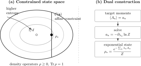
Left: an affine constraint selects a convex family of compatible states, and the highest entropy contour touching that family identifies $\rho_\star$. Right: the dual calculation chooses multipliers so that the exponential state reproduces the target moments.

For a finite-dimensional Hilbert space:

• the set of density operators is compact;
• affine equality constraints define a closed feasible set;
• $\mathsf S(\rho)$ is continuous;
• therefore a maximizer exists whenever the constraints are feasible;
• strict concavity makes the maximizing state unique.

Uniqueness of the state does not imply uniqueness of every multiplier. Redundant constraint operators can give different multiplier vectors that produce the same exponent up to a multiple of the identity.

General Finite-Dimensional Problem

Let $A_1,\ldots,A_m$ be Hermitian operators on a $d$-dimensional Hilbert space. Define the feasible set

$$\mathcal C(\mathbf a) = \left\{ \rho\geq0: \operatorname{Tr}\rho=1,\ \operatorname{Tr}(\rho A_a)=a_a \right\}.$$

The target vector

$$\mathbf a = (a_1,\ldots,a_m)$$

must lie in the convex set of attainable expectation values. If $\mathcal C(\mathbf a)$ is empty, no inference method can produce a state satisfying all constraints exactly.

Introduce the generalized potential

$$K(\boldsymbol\lambda) = \sum_{a=1}^{m} \lambda_aA_a,$$

the partition function

$$Z(\boldsymbol\lambda) = \operatorname{Tr} e^{-K(\boldsymbol\lambda)},$$

and the exponential state

$$\sigma_{\boldsymbol\lambda} = \frac{ e^{-K(\boldsymbol\lambda)} }{ Z(\boldsymbol\lambda) }.$$

The central task is to find multipliers satisfying

$$\operatorname{Tr} \left( \sigma_{\boldsymbol\lambda}A_a \right) = a_a$$

for every independent constraint.

Relative-Entropy Proof of Optimality

The cleanest proof avoids delicate variations at zero eigenvalues. For any feasible $\rho$, consider the quantum relative entropy

$$D \left( \rho\Vert\sigma_{\boldsymbol\lambda} \right) = \operatorname{Tr} \left[ \rho \left( \ln\rho - \ln\sigma_{\boldsymbol\lambda} \right) \right].$$

Because

$$\ln\sigma_{\boldsymbol\lambda} = - \sum_a\lambda_aA_a - \ln Z,$$

one obtains

$$\begin{aligned} D \left( \rho\Vert\sigma_{\boldsymbol\lambda} \right) ={}& - \mathsf S(\rho) \\ &+ \sum_a \lambda_a a_a + \ln Z. \end{aligned}$$

Nonnegativity of relative entropy gives the upper bound

$$\mathsf S(\rho) \leq \ln Z(\boldsymbol\lambda) + \sum_a\lambda_a a_a.$$

If $\sigma_{\boldsymbol\lambda}$ itself satisfies the constraints, then

$$\mathsf S \left( \sigma_{\boldsymbol\lambda} \right) = \ln Z(\boldsymbol\lambda) + \sum_a\lambda_a a_a,$$

so every feasible state obeys

$$\mathsf S(\rho) \leq \mathsf S \left( \sigma_{\boldsymbol\lambda} \right).$$

Equality holds only when

$$D \left( \rho\Vert\sigma_{\boldsymbol\lambda} \right) = 0,$$

which implies $\rho=\sigma_{\boldsymbol\lambda}$. This proves both optimality and uniqueness.

The same calculation gives the exact entropy-gap identity

$$\mathsf S \left( \rho_\star \right) - \mathsf S(\rho) = D \left( \rho\Vert\rho_\star \right)$$

for every state $\rho$ sharing the retained expectation values with a full-rank exponential maximizer $\rho_\star$.

Lagrange-Multiplier Derivation

For an interior solution, vary the functional

$$\begin{aligned} \mathcal L[\rho] ={}& - \operatorname{Tr}(\rho\ln\rho) \\ &- \alpha \left( \operatorname{Tr}\rho-1 \right) \\ &- \sum_a\lambda_a \left[ \operatorname{Tr}(\rho A_a)-a_a \right]. \end{aligned}$$

At a full-rank $\rho$,

$$\delta\mathsf S = - \operatorname{Tr} \left[ \delta\rho \left( \ln\rho+\mathbb I \right) \right].$$

Stationarity under arbitrary Hermitian variations gives

$$\ln\rho = - (1+\alpha)\mathbb I - \sum_a\lambda_aA_a.$$

Exponentiating,

$$\rho = e^{-(1+\alpha)} \exp \left( - \sum_a\lambda_aA_a \right).$$

Normalization fixes

$$e^{1+\alpha} = Z(\boldsymbol\lambda),$$

and hence

$$\rho = \frac{ \exp\left(-\sum_a\lambda_aA_a\right) }{ Z(\boldsymbol\lambda) }.$$

This stationarity derivation is useful, but it assumes the solution lies in the interior of state space. The relative-entropy proof also makes clear why the stationary state is the global maximum.

Determining the Multipliers

Define

$$\psi(\boldsymbol\lambda) = \ln Z(\boldsymbol\lambda).$$

Then

$$\frac{\partial\psi}{\partial\lambda_a} = - \operatorname{Tr} \left( \rho_{\boldsymbol\lambda}A_a \right) = - \langle A_a\rangle_{\boldsymbol\lambda}.$$

This derivative remains valid when the constraint operators do not commute. One uses the operator identity

$$\frac{\partial e^{-K}}{\partial\lambda_a} = - \int_0^1 e^{-(1-s)K} A_a e^{-sK} \,ds$$

and cyclicity of the trace.

The multiplier equations are therefore

$$\nabla_{\boldsymbol\lambda} \psi(\boldsymbol\lambda) = - \mathbf a.$$

For centered operators

$$\Delta A_a = A_a-\langle A_a\rangle\mathbb I,$$

the Hessian is the Kubo–Mori covariance matrix

$$\frac{\partial^2\psi} {\partial\lambda_a\partial\lambda_b} = \int_0^1 \operatorname{Tr} \left( \rho^s \Delta A_a \rho^{1-s} \Delta A_b \right) ds.$$

It is positive semidefinite, so $\psi$ is convex. If all constrained operators commute with $\rho$, this reduces to the ordinary covariance

$$\frac{\partial^2\psi} {\partial\lambda_a\partial\lambda_b} = \langle \Delta A_a\Delta A_b \rangle.$$

Zero modes of the covariance matrix signal redundant constraints or directions that do not change the state.

Entropy as a Dual Function

For any multiplier vector, define

$$g(\boldsymbol\lambda;\mathbf a) = \psi(\boldsymbol\lambda) + \boldsymbol\lambda\mathbin{\cdot}\mathbf a.$$

The relative-entropy inequality shows that $g$ is an upper bound on the entropy of every feasible state. Under regularity conditions,

$$\mathsf S_{\max}(\mathbf a) = \inf_{\boldsymbol\lambda} \left[ \psi(\boldsymbol\lambda) + \boldsymbol\lambda\mathbin{\cdot}\mathbf a \right].$$

At an interior optimum,

$$\frac{\partial g}{\partial\lambda_a} = 0$$

is exactly the moment-matching equation. The envelope relation is

$$\frac{\partial\mathsf S_{\max}} {\partial a_a} = \lambda_a.$$

Thus the Lagrange multipliers are variables conjugate to the retained expectation values. If the Kubo–Mori covariance matrix $G$ is invertible,

$$\frac{\partial\lambda_a}{\partial a_b} = - \left( G^{-1} \right)_{ab},$$

which expresses concavity of the optimized entropy.

Thermodynamic Legendre transforms are concrete realizations of this dual structure. Thermodynamic Potentials owns their natural variables, differentials, and Maxwell relations.

Canonical State from Mean Energy

Work in a fixed particle-number sector with Hamiltonian $H_N$. Impose

$$\operatorname{Tr}\rho=1, \qquad \operatorname{Tr}(\rho H_N)=U.$$

There is one nontrivial multiplier:

$$\rho_\beta = \frac{ e^{-\beta H_N} }{ Z_N(\beta) }, \qquad Z_N(\beta) = \operatorname{Tr}_{\mathcal H_N} e^{-\beta H_N}.$$

The target energy determines $\beta$ through

$$U = - \frac{\partial\ln Z_N}{\partial\beta}.$$

At this stage, $\beta$ is an inverse-energy Lagrange multiplier. Its thermodynamic interpretation follows from

$$\mathsf S_{\max}(U) = \ln Z_N+\beta U$$

and

$$\frac{\partial S_{\max}}{\partial U} = k_{\mathrm B}\beta.$$

Comparing with

$$\left( \frac{\partial S}{\partial U} \right)_{V,N} = \frac{1}{T}$$

identifies

$$\beta = \frac{1}{k_{\mathrm B}T}.$$

The variational principle can equivalently be written at fixed temperature. Define

$$\mathcal F_T(\rho) = \operatorname{Tr}(\rho H_N) - T S(\rho).$$

Then

$$\mathcal F_T(\rho) - \mathcal F_T(\rho_\beta) = k_{\mathrm B}T D(\rho\Vert\rho_\beta) \geq0.$$

Thus the Gibbs state uniquely minimizes the nonequilibrium free-energy functional. The Canonical Ensemble owns the reservoir argument, fixed-$T,N,V$ thermodynamics, and energy-fluctuation formulas.

Grand-Canonical State from Energy and Number

Now allow the state space to include multiple number sectors and impose

$$\operatorname{Tr}(\rho H)=U, \qquad \operatorname{Tr}(\rho N)=\overline N.$$

Using independent dimensionless multipliers $\beta$ and $\gamma$ gives

$$\rho_{\beta,\gamma} = \frac{ e^{-\beta H-\gamma N} }{ \mathcal Z(\beta,\gamma) },$$

with

$$\mathcal Z(\beta,\gamma) = \operatorname{Tr} e^{-\beta H-\gamma N}.$$

The independent moment equations are

$$U = - \left( \frac{\partial\ln\mathcal Z}{\partial\beta} \right)_{\gamma}, \qquad \overline N = - \left( \frac{\partial\ln\mathcal Z}{\partial\gamma} \right)_{\beta}.$$

For an equilibrium conserved particle number, write

$$\gamma = - \beta\mu.$$

Then

$$\rho_{\beta,\mu} = \frac{ e^{-\beta(H-\mu N)} }{ \Xi(\beta,\mu) }, \qquad \Xi = \operatorname{Tr} e^{-\beta(H-\mu N)}.$$

The entropy at the matched constraints is

$$S = k_{\mathrm B} \left[ \ln\Xi + \beta \left( U-\mu\overline N \right) \right].$$

After the change of variables from $(\beta,\gamma)$ to $(\beta,\mu)$,

$$- \left( \frac{\partial\ln\Xi}{\partial\beta} \right)_{\mu} = U-\mu\overline N,$$

whereas

$$\frac{1}{\beta} \left( \frac{\partial\ln\Xi}{\partial\mu} \right)_{\beta} = \overline N.$$

Holding $\gamma=-\beta\mu$ fixed is not the same derivative as holding $\mu$ fixed.

The algebraic maximization can constrain any Hermitian $N$. Calling its multiplier a thermodynamic chemical potential requires additional physics, normally including

$$[H,N]=0$$

and a mechanism that exchanges the conserved quantity. Chemical Potential owns that physical interpretation, while the Grand-Canonical Ensemble owns the Fock-space trace and number-sector statistics.

Exact Constraints Are Not Mean Constraints

Suppose $P$ projects onto an allowed subspace of dimension

$$r = \operatorname{Tr}P.$$

Imposing the exact support condition

$$P\rho P = \rho$$

does not introduce a finite expectation-value multiplier. The maximum-entropy state on the subspace is

$$\rho_P = \frac{P}{r}.$$

Indeed, for any state supported in $P\mathcal H$,

$$D \left( \rho\middle\Vert\frac{P}{r} \right) = \ln r-\mathsf S(\rho) \geq0.$$

For an energy-shell projector $P_{E,\Delta}$, this gives

$$\rho_{\mathrm{mc}} = \frac{ P_{E,\Delta} }{ \operatorname{Tr}P_{E,\Delta} }.$$

By contrast, fixing only $\langle H\rangle=U$ allows support on many energies and produces $e^{-\beta H}/Z$.

Constraint	What is exact?	Typical maximizing state
$P\rho P=\rho$	allowed subspace	uniform on that subspace
$\langle H\rangle=U$	mean energy	canonical exponential state
$N\rho=N_0\rho$	number sector	state restricted to $\mathcal H_{N_0}$
$\langle N\rangle=\overline N$	mean number	state spanning number sectors

The Microcanonical Ensemble owns energy-window conventions and shell thermodynamics.

Interior and Boundary Solutions

For finite multipliers in finite dimension,

$$\rho_{\boldsymbol\lambda} \propto e^{-K(\boldsymbol\lambda)}$$

is full rank. Therefore a rank-deficient maximizer cannot generally be represented with finite multipliers.

Consider a Hamiltonian with lowest energy $E_0$ and ground-space projector $P_0$. The boundary target

$$\langle H\rangle = E_0$$

forces the state into the ground space. Maximum entropy gives

$$\rho_\star = \frac{ P_0 }{ \operatorname{Tr}P_0 }.$$

It is reached as the limit

$$\rho_\star = \lim_{\beta\to+\infty} \frac{e^{-\beta H}}{Z(\beta)}.$$

For a nondegenerate ground state this limit is pure; for a degenerate ground space it is the uniform mixture unless further constraints distinguish ground states.

Boundary behavior matters numerically. A solver may send one or more multipliers toward infinity rather than converge to a finite point. That can be the correct signal of a rank-deficient optimum rather than a failure of the entropy principle.

Feasibility and Redundant Constraints

Before solving for multipliers, check whether the target moments are possible. For one Hermitian operator $A$,

$$\lambda_{\min}(A) \leq \langle A\rangle \leq \lambda_{\max}(A).$$

With several operators, separate interval checks are necessary but may not be sufficient. Their joint expectation-value region can impose additional inequalities.

Constraints are redundant when one retained operator is an affine combination of the others. If

$$A_2 = cA_1+d\mathbb I,$$

then every normalized state satisfies

$$\langle A_2\rangle = c\langle A_1\rangle+d.$$

If the targets violate this relation, the feasible set is empty. If they obey it, the maximizing state is unique but the pair $(\lambda_1,\lambda_2)$ is not: only the combination multiplying $A_1$ affects the normalized state.

In computations, remove affine redundancies or use a gauge convention before inverting a susceptibility matrix.

Classical Reduction

If all constrained operators commute, choose a common eigenbasis:

$$A_a|i\rangle = a_{a,i}|i\rangle.$$

The exponential state is diagonal,

$$\rho_\star = \sum_i p_i|i\rangle\langle i|,$$

with

$$p_i = \frac{ e^{-\sum_a\lambda_a a_{a,i}} }{ \sum_j e^{-\sum_a\lambda_a a_{a,j}} }.$$

The quantum problem then reduces to the classical maximum-Shannon-entropy distribution over the joint eigenvalues. Within an unresolved degenerate joint eigenspace, the maximizing state is proportional to the identity.

Off-diagonal coherence cannot improve the entropy while preserving only commuting moments. Dephasing in the common eigenbasis preserves those moments and cannot decrease the entropy.

Noncommuting Constraints

Expectation values of noncommuting observables can be constrained simultaneously. They need not possess simultaneous sharp values. The finite-dimensional variational answer remains

$$\rho_\star = \frac{ e^{-\sum_a\lambda_aA_a} }{ Z },$$

where the exponential is taken after forming the operator sum.

In general,

$$e^{-\lambda A-\eta B} \neq e^{-\lambda A}e^{-\eta B}$$

when $[A,B]\neq0$. Product factorization would change the state and can even destroy Hermiticity if used carelessly.

The inferred state need not commute with each constrained observable:

$$[\rho_\star,A_a] \neq 0$$

can occur even though all target expectation values are reproduced. Ordinary covariances must then be replaced by the Kubo–Mori matrix in multiplier-response formulas.

There is also a physical distinction between inference and equilibrium. If a constrained charge fails to commute with $H$, the exponential state may fail to be stationary:

$$[H,\rho_\star] \neq 0.$$

Noncommuting conserved charges require a more careful thermodynamic framework, including what conservation means for the composite system and which exchanges are allowed. The formal maximum-entropy calculation is valid more broadly than the equilibrium interpretation attached to it.

Example: One Qubit Constraint

Write a qubit state as

$$\rho = \frac{1}{2} \left( \mathbb I + \mathbf r\mathbin{\cdot}\boldsymbol\sigma \right), \qquad |\mathbf r|\leq1.$$

Suppose the only measured moment is

$$\langle\sigma_z\rangle = m, \qquad -1\leq m\leq1.$$

The constraint fixes $r_z=m$ but leaves $r_x$ and $r_y$ unknown. The eigenvalues are

$$p_\pm = \frac{1\pm|\mathbf r|}{2},$$

and the entropy decreases as $|\mathbf r|$ increases away from zero. For fixed $r_z=m$, the smallest possible Bloch-vector length is obtained at

$$r_x=r_y=0.$$

Therefore

$$\rho_\star = \frac{1}{2} \left( \mathbb I+m\sigma_z \right).$$

The same state has exponential form

$$\rho_\star = \frac{ e^{-\lambda\sigma_z} }{ 2\cosh\lambda },$$

with

$$m = - \tanh\lambda, \qquad \lambda = - \operatorname{artanh}m.$$

At $m=0$, no polarization is known and $\rho_\star=\mathbb I/2$. At $m=\pm1$, the target lies on the boundary and the maximizing state is pure; the multiplier diverges.

Example: Two Noncommuting Qubit Constraints

Now retain

$$\langle\sigma_x\rangle=x, \qquad \langle\sigma_z\rangle=z.$$

Feasibility requires

$$x^2+z^2 \leq 1.$$

The unmeasured component $r_y$ only increases $|\mathbf r|$ and lowers the entropy. Hence

$$\rho_\star = \frac{1}{2} \left( \mathbb I+x\sigma_x+z\sigma_z \right).$$

Let

$$r = \sqrt{x^2+z^2}, \qquad \widehat{\mathbf r} = \frac{(x,0,z)}{r}$$

for $r>0$. Then

$$\rho_\star = \frac{ \exp \left[ \operatorname{artanh}(r) \, \widehat{\mathbf r} \mathbin{\cdot} \boldsymbol\sigma \right] }{ 2\cosh \left[ \operatorname{artanh}(r) \right] }.$$

This is of the required form with a multiplier vector antiparallel to the retained Bloch vector. The noncommutation

$$[\sigma_x,\sigma_z] = - 2i\sigma_y$$

does not obstruct expectation-value inference. It does obstruct interpreting $x$ and $z$ as simultaneously sharp eigenvalues.

Maximum Entropy Relative to a Prior State

Plain maximum entropy uses the maximally mixed state as its implicit finite-dimensional reference because

$$D \left( \rho\middle\Vert\frac{\mathbb I}{d} \right) = \ln d-\mathsf S(\rho).$$

If a full-rank reference state $\sigma$ represents information that should be retained before imposing new moments, a natural generalization minimizes

$$D(\rho\Vert\sigma)$$

over the feasible set. The interior solution is

$$\rho_\star = \frac{ \exp \left( \ln\sigma-\sum_a\lambda_aA_a \right) }{ \operatorname{Tr} \exp \left( \ln\sigma-\sum_a\lambda_aA_a \right) }.$$

When $\sigma$ commutes with all $A_a$, this resembles a classical reweighting. In the noncommuting case,

$$\exp \left( \ln\sigma-\lambda A \right)$$

must not be replaced by $\sigma e^{-\lambda A}$.

This relative-entropy projection makes “least biased” explicitly conditional on a reference. It is also indispensable in infinite-dimensional settings, where no normalized state proportional to the identity may exist.

Constraint-Based Coarse Graining

Suppose an exact state $\rho$ is replaced by the maximum-entropy state that preserves selected moments:

$$\operatorname{Tr}(\rho_\star A_a) = \operatorname{Tr}(\rho A_a).$$

Then

$$\mathsf S(\rho_\star) \geq \mathsf S(\rho).$$

The entropy increase measures distinctions discarded by retaining only those moments. For a full-rank exponential maximizer,

$$\mathsf S(\rho_\star) - \mathsf S(\rho) = D(\rho\Vert\rho_\star).$$

This replacement is generally nonlinear in $\rho$ because the multipliers depend nonlinearly on the retained expectation values. It should not automatically be treated as a physical quantum channel or a dynamical law. Entropy in Quantum Statistical Mechanics owns the broader distinctions among thermal, entanglement, diagonal, and coarse-grained entropies.

What the Principle Does Not Prove

It does not choose the constraints

The analyst must justify why energy, particle number, magnetization, local densities, or other moments are retained. Omitting an exactly conserved quantity can give the wrong equilibrium family; integrable generalized ensembles make this constraint-selection problem especially sharp.

It does not prove thermalization

Maximization compares states at one time. It supplies no equation of motion and no relaxation timescale. Relaxation and Thermalization owns the closed-system dynamical tests; ergodicity, eigenstate thermalization, integrability, and coupling to a bath remain additional questions.

It does not derive a reservoir model

A bath derivation explains why particular intensive variables are controlled and when the reduced state is approximately Gibbsian. Maximum entropy derives the same exponential form from different premises.

It does not establish ensemble equivalence

Microcanonical, canonical, and grand-canonical states can remain different at finite size and for global fluctuations. Their thermodynamic-limit agreement requires additional hypotheses, developed in Ensemble Equivalence.

It does not make omitted observables physically zero

The inferred state predicts values for unconstrained observables, often zero by symmetry. That means zero is the maximum-entropy assignment under the retained information, not that every compatible microscopic preparation has that value.

It does not remove trace-domain choices

Maximizing over a fixed-$N$ Hilbert space and maximizing over Fock space are different problems even if the exponent looks similar. The allowed state space is part of the input.

Infinite-Dimensional Caveats

Compactness and a normalized maximally mixed state are lost in infinite dimension. Several failures can occur:

• $Z(\boldsymbol\lambda)$ may diverge;
• the target moments may not be finite;
• entropy may be unbounded above on the feasible set;
• an entropy supremum may exist without being attained;
• unbounded constraint operators require domain control;
• continuum volume factors may make traces infinite.

For a free particle on the infinite line,

$$\operatorname{Tr} e^{-\beta p^2/(2m)}$$

diverges because of the infinite spatial volume. A finite box, a density per unit volume, or another regularization must be specified before normalizing a canonical state.

Even when $Z$ is finite, differentiating it requires the relevant operator moments to exist. One should establish trace-class and differentiability conditions rather than importing finite-matrix arguments unchanged.

A Reliable Workflow

1. Specify the state space. Name the Hilbert space, superselection sector, volume regulator, and trace domain.
2. Separate exact from mean constraints. Exact support, exact charge sectors, and expectation values lead to different feasible sets.
3. Check feasibility. Verify spectral bounds and joint compatibility of target moments.
4. Remove redundancies. Identify affine relations among constraint operators.
5. Use dimensionless multipliers. Track physical units before naming a multiplier temperature or chemical potential.
6. Check normalization. Confirm that the exponential is trace class and $Z<\infty$.
7. Match the moments. Solve $-\partial_{\lambda_a}\ln Z=a_a$ with the correct variables held fixed.
8. Verify global optimality. Use the relative-entropy identity, not stationarity alone.
9. Inspect boundary behavior. Diverging multipliers can represent a legitimate rank-deficient optimum.
10. Justify the physics. Explain why the constraints are conserved, controlled, or experimentally known.
11. Keep inference separate from dynamics. Add a thermalization or bath argument when the claim requires one.

Canonical Boundaries

This page owns:

• the general constrained von Neumann entropy optimization;
• the exponential-family derivation and relative-entropy proof;
• multiplier matching, convex duality, and Kubo–Mori response;
• exact-support versus expectation-value constraints;
• feasibility, redundancy, interior, and boundary solutions;
• the inference meaning and its limitations;
• the extension to noncommuting moments and prior states.

Other pages own:

• operator properties and spectral examples of Gibbs states: Thermal Density Operators;
• fixed-$T,N,V$ thermodynamics and reservoir derivation: Canonical Ensemble;
• Fock-space structure and number fluctuations: Grand-Canonical Ensemble;
• entropy interpretations and coarse-graining taxonomy: Entropy in Quantum Statistical Mechanics;
• chemical-potential definitions and conserved-number physics: Chemical Potential;
• equilibrium fluctuation identities and static susceptibility applications: Fluctuations and Susceptibilities;
• dynamical equilibration, entropy production, and operational work: Quantum Thermodynamics.

Common Mistakes

• Treating an exact energy shell as though it were only a mean-energy constraint.
• Omitting positivity and optimizing over arbitrary trace-one Hermitian operators.
• Calling a Lagrange multiplier temperature or chemical potential before establishing the thermodynamic interpretation.
• Choosing multipliers independently of the target expectation values.
• Proving stationarity but not global maximality.
• Assuming every maximizing state has finite multipliers.
• Ignoring infeasible or redundant constraints.
• Factoring an exponential of noncommuting operators.
• Treating a mean value of a noncommuting observable as a sharp simultaneous value.
• Using a particle-number multiplier as a chemical potential when the proposed number is not conserved.
• Confusing a maximum-entropy assignment with a dynamical thermalization theorem.
• Forgetting that the trace domain determines whether the state is canonical or grand canonical.
• Assuming predictions for omitted observables describe every compatible preparation.
• Invoking a uniform prior in an infinite-dimensional space without a regulator.
• Dropping $k_{\mathrm B}$ when converting dimensionless entropy derivatives into thermodynamic ones.

Exercises

The maximally mixed state

Show that $\mathbb I/d$ uniquely maximizes von Neumann entropy on a $d$-dimensional Hilbert space when normalization is the only constraint.

Solution

For any density operator $\rho$,

$$\begin{aligned} D \left( \rho\middle\Vert\frac{\mathbb I}{d} \right) &= \operatorname{Tr} \left[ \rho \left( \ln\rho+\ln d \right) \right] \\ &= \ln d-\mathsf S(\rho). \end{aligned}$$

Relative entropy is nonnegative, so

$$\mathsf S(\rho) \leq \ln d.$$

Equality holds only if

$$\rho = \frac{\mathbb I}{d}.$$

Entropy gap to an exponential state

Let

$$\rho_\star = \frac{ e^{-\sum_a\lambda_aA_a} }{ Z }$$

match the same expectation values $\langle A_a\rangle=a_a$ as a state $\rho$. Prove

$$\mathsf S(\rho_\star) - \mathsf S(\rho) = D(\rho\Vert\rho_\star).$$

Solution

Use

$$\ln\rho_\star = - \sum_a\lambda_aA_a - \ln Z.$$

Then

$$\begin{aligned} D(\rho\Vert\rho_\star) ={}& \operatorname{Tr}(\rho\ln\rho) \\ &+ \sum_a\lambda_a \operatorname{Tr}(\rho A_a) + \ln Z \\ ={}& - \mathsf S(\rho) + \sum_a\lambda_aa_a + \ln Z. \end{aligned}$$

For $\rho_\star$ itself,

$$\mathsf S(\rho_\star) = \sum_a\lambda_aa_a+\ln Z.$$

Substitution gives the required identity. Nonnegativity of $D$ proves that $\rho_\star$ is the global maximum.

Qubit polarization

Maximize the entropy of a qubit subject to

$$\langle\sigma_z\rangle = \frac{1}{2}.$$

Find the density matrix, its entropy, and the multiplier $\lambda$ in

$$\rho_\star \propto e^{-\lambda\sigma_z}.$$

Solution

The maximum-entropy state has no unconstrained transverse Bloch components:

$$\rho_\star = \frac{1}{2} \left( \mathbb I+\frac{1}{2}\sigma_z \right).$$

In the $\sigma_z$ basis,

$$\rho_\star = \begin{pmatrix} 3/4&0\\ 0&1/4 \end{pmatrix}.$$

Its dimensionless entropy is

$$\mathsf S(\rho_\star) = - \frac{3}{4}\ln\frac{3}{4} - \frac{1}{4}\ln\frac{1}{4}.$$

Because $m=-\tanh\lambda$,

$$\lambda = - \operatorname{artanh} \left( \frac{1}{2} \right) = - \frac{1}{2}\ln3.$$

Exact ground energy

A finite-dimensional Hamiltonian has ground energy $E_0$ with degeneracy $g_0$. Maximize entropy subject to the exact mean-energy target $\langle H\rangle=E_0$. Explain why the answer is not a finite-temperature Gibbs state.

Solution

Since $H-E_0\mathbb I\geq0$,

$$\operatorname{Tr} \left[ \rho \left( H-E_0\mathbb I \right) \right] = 0$$

forces $\rho$ to have support only in the kernel of $H-E_0\mathbb I$, namely the ground space. Entropy is maximized uniformly on that $g_0$-dimensional subspace:

$$\rho_\star = \frac{P_0}{g_0}, \qquad \mathsf S(\rho_\star) = \ln g_0.$$

Every finite $\beta$ gives a full-rank Gibbs state and assigns nonzero weight to excited levels. The solution is the boundary limit

$$\rho_\star = \lim_{\beta\to+\infty} \frac{e^{-\beta H}}{Z(\beta)}.$$

Grand-canonical multiplier signs

Maximize entropy under fixed $U=\langle H\rangle$ and $\overline N=\langle N\rangle$ using independent multipliers $\beta$ and $\gamma$. Derive the state, set $\gamma=-\beta\mu$, and show what $-\partial_\beta\ln\Xi$ gives when $\mu$ is held fixed.

Solution

The independent-multiplier solution is

$$\rho_{\beta,\gamma} = \frac{ e^{-\beta H-\gamma N} }{ \mathcal Z(\beta,\gamma) }.$$

With

$$\gamma=-\beta\mu,$$

this becomes

$$\rho_{\beta,\mu} = \frac{ e^{-\beta(H-\mu N)} }{ \Xi(\beta,\mu) }.$$

At fixed $\mu$,

$$\begin{aligned} - \left( \frac{\partial\ln\Xi}{\partial\beta} \right)_\mu &= \left\langle H-\mu N \right\rangle \\ &= U-\mu\overline N. \end{aligned}$$

It does not equal $U$ unless $\mu\overline N=0$. At fixed independent $\gamma$, one instead has

$$- \left( \frac{\partial\ln\mathcal Z}{\partial\beta} \right)_\gamma = U.$$

Two noncommuting qubit moments

Suppose

$$\langle\sigma_x\rangle = \frac{1}{3}, \qquad \langle\sigma_z\rangle = \frac{2}{3}.$$

Find the maximum-entropy state and verify that it is positive.

Solution

Maximum entropy sets the unconstrained component $\langle\sigma_y\rangle$ to zero:

$$\rho_\star = \frac{1}{2} \left( \mathbb I + \frac{1}{3}\sigma_x + \frac{2}{3}\sigma_z \right).$$

In the $\sigma_z$ basis,

$$\rho_\star = \begin{pmatrix} 5/6&1/6\\ 1/6&1/6 \end{pmatrix}.$$

The Bloch-vector length is

$$r = \frac{\sqrt5}{3} < 1,$$

so the eigenvalues

$$p_\pm = \frac{1}{2} \left( 1\pm\frac{\sqrt5}{3} \right)$$

are both positive. The state is therefore a valid full-rank density operator even though $\sigma_x$ and $\sigma_z$ do not commute.

Redundant constraints

Let $A_2=2A_1+3\mathbb I$. Determine the feasibility condition on targets $(a_1,a_2)$ and show why the multipliers in

$$\rho \propto e^{-\lambda_1A_1-\lambda_2A_2}$$

are not unique.

Solution

Every normalized state satisfies

$$\langle A_2\rangle = 2\langle A_1\rangle+3,$$

so feasibility requires

$$a_2 = 2a_1+3.$$

The exponent can be rearranged as

$$\begin{aligned} - \lambda_1A_1 - \lambda_2A_2 ={}& - \left( \lambda_1+2\lambda_2 \right) A_1 \\ &- 3\lambda_2\mathbb I. \end{aligned}$$

The identity term cancels from the normalized density operator. Therefore the state depends only on

$$\lambda_{\mathrm{eff}} = \lambda_1+2\lambda_2.$$

Infinitely many multiplier pairs give the same unique maximum-entropy state.

Cross-Links

• Start with the ensemble-level comparison in Statistical Ensembles Overview.
• Review the operator exponential and spectral form in Thermal Density Operators.
• Compare exact energy-shell information in Microcanonical Ensemble.
• Use Canonical Ensemble for fixed-number thermodynamics.
• Use Grand-Canonical Ensemble for Fock-space construction and number fluctuations.
• See Relative Entropy for positivity, support conditions, and data-processing properties.
• Keep state inference distinct from dynamical and operational questions in Quantum Thermodynamics.

References

• E. T. Jaynes, “Information Theory and Statistical Mechanics”, Physical Review 106, 620–630 (1957).
• E. T. Jaynes, “Information Theory and Statistical Mechanics. II”, Physical Review 108, 171–190 (1957).
• E. H. Wichmann, “Density Matrices Arising from Incomplete Measurements”, Journal of Mathematical Physics 4, 884–896 (1963).
• A. Wehrl, “General Properties of Entropy”, Reviews of Modern Physics 50, 221–260 (1978).
• R. Balian, From Microphysics to Macrophysics: Methods and Applications of Statistical Physics, volumes I and II, Springer (1991–1992), chapters on statistical inference and equilibrium ensembles.
• D. Petz, Quantum Information Theory and Quantum Statistics, Springer (2008), chapters on entropy, relative entropy, and exponential families.
• N. Yunger Halpern, P. Faist, J. Oppenheim, and A. Winter, “Microcanonical and Resource-Theoretic Derivations of the Thermal State of a Quantum System with Noncommuting Charges”, Nature Communications 7, 12051 (2016).
• R. K. Pathria and P. D. Beale, Statistical Mechanics, 4th ed., Elsevier (2021), chapters 2–5.