Relaxation and Thermalization

An isolated quantum system evolves unitarily. Its exact state does not forget its initial condition, its von Neumann entropy does not increase, and a finite system generally recurs. Yet local observables can settle near reproducible values, small subsystems can become nearly indistinguishable from thermal states, and equilibrium statistical mechanics can predict late-time measurements with striking accuracy.

The resolution is operational. Closed-system thermalization is not convergence of the global wavefunction to a mixed state. It is a two-stage statement about a declared class of probes:

$$\boxed{ \begin{gathered} \text{unitary dynamics} \\ \Downarrow \\ \text{local equilibration}, \\ \text{equilibrated values} \\ \Downarrow \\ \text{constrained thermal ensemble}. \end{gathered} }$$

The first arrow is largely about dephasing and suppressed temporal fluctuations. The second is the genuinely thermal identification. Either arrow can fail.

For a subsystem $A$, the central error decomposition is

$$\begin{aligned} D\left( \rho_A(t), \rho_A^{\mathrm{th}} \right) \le{}& D\left( \rho_A(t), \omega_A \right) \\ & + D\left( \omega_A, \rho_A^{\mathrm{th}} \right), \end{aligned}$$

where $\omega$ is the dephased state and

$$D(\rho,\sigma) = \frac{1}{2} \|\rho-\sigma\|_1$$

is trace distance. The first term is the dynamical equilibration error. The second is the ensemble-identification error. Calling the first term small does not make the second small.

Scope and Canonical Ownership

This page owns the closed-system bridge from unitary dynamics to thermal behavior:

• relaxation, equilibration, and thermalization as operational claims;
• exact dephasing to the diagonal ensemble;
• effective dimension and energy-gap conditions for small temporal fluctuations;
• local-observable and reduced-state criteria;
• the separation between global purity and local thermal appearance;
• selection of microcanonical, canonical, charge-constrained, or generalized candidates;
• the roles of exact symmetries, conserved densities, and hydrodynamic slow modes;
• timescales, recurrences, order of limits, and evidence standards;
• common mechanisms and controlled failure modes.

Canonical neighbors retain their own derivations:

• Nonequilibrium Overview owns the chapter-wide vocabulary and map of thermalizing, integrable, localized, constrained, and driven regimes.
• Quantum Quenches owns the sudden-switch protocol, final-energy distribution, spreading, entanglement growth, and Loschmidt amplitude.
• Microcanonical Ensemble and Canonical Ensemble own equilibrium state definitions.
• Ensemble Equivalence owns thermodynamic-limit comparison among equilibrium ensembles.
• Maximum Entropy Principle owns inference from stated constraints; it does not supply dynamics.
• Time-Dependent Correlations owns two-time functions and stationary spectral relations.
• Steady States and Relaxation owns attractors and relaxation modes of Markovian open-system generators.
• Quantum Thermalization is the quantum-matter bridge for platform ledgers, independently fixed ensembles, experiment-specific observables, and closed-versus-open evidence audits.

The next pages of this chapter own the detailed eigenstate thermalization ansatz, generalized Gibbs ensembles, many-body localization, prethermalization, many-body quantum chaos, and scrambling and OTOCs. This page states only the interfaces needed to judge a thermalization claim.

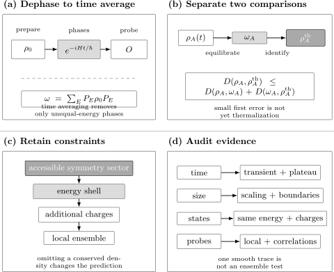
Closed-system thermalization requires more than a smooth time trace. One first tests equilibration to the dephased state, then tests that state against an ensemble retaining every relevant constraint. Time windows, size scaling, initial-state variation, and multiple probes are part of the claim.

Exact Unitary Starting Point

Let $H$ be time independent after the preparation. In finite dimension, write its spectral resolution using distinct energies:

$$H = \sum_E E P_E.$$

The state evolves as

$$\rho(t) = e^{-iHt/\hbar} \rho_0 e^{iHt/\hbar}.$$

For a bounded observable $O$,

$$\langle O(t)\rangle = \sum_{E,E'} e^{-i(E-E')t/\hbar} \operatorname{Tr} \left( P_E\rho_0P_{E'}O \right).$$

The time dependence is carried entirely by unequal-energy phases. The exact state retains them; a restricted observable may cease to resolve their coherent sum.

The dephased state

The infinite-time average is

$$\begin{aligned} \omega &\equiv \overline{\rho(t)}, \\ \omega &= \lim_{T\to\infty} \frac{1}{T} \int_0^T \rho(t)\,dt, \\ \omega &= \sum_E P_E\rho_0P_E. \end{aligned}$$

Therefore

$$\overline{\langle O(t)\rangle} = \operatorname{Tr}(\omega O).$$

The projector form matters. Coherences inside a degenerate energy eigenspace have no relative phase and survive. “Delete every off-diagonal matrix element in a chosen eigenbasis” is basis dependent and generally wrong in a degenerate subspace.

The dephased state is also called the diagonal ensemble when a nondegenerate energy basis is understood. It stores every populated final-energy sector and, within degeneracies, all stationary coherence. It is not generally a microcanonical, canonical, or maximum-entropy state.

Time average is not convergence

A time average can exist while the instantaneous signal keeps making large excursions. Define

$$\delta_O(t) \equiv \langle O(t)\rangle - \operatorname{Tr}(\omega O)$$

and the infinite-time variance

$$\sigma_O^2 \equiv \overline{ |\delta_O(t)|^2 }.$$

Small $\sigma_O$ means the observable remains near its time average for most times. The equality

$$\overline{\delta_O(t)}=0$$

alone says nothing about fluctuation size.

Relaxation, Equilibration, and Thermalization

Relaxation

Relaxation describes an observable or reduced state approaching a late-time regime after a transient. A complete statement names:

• the observable or subsystem;
• the proposed late-time value or manifold;
• the time window;
• the relaxation scale;
• residual oscillations or long-time tails;
• finite-size and boundary effects.

Relaxation need not be monotonic or exponential. Damped oscillations, algebraic decay, stretched exponentials, plateaus, and multistage relaxation are all possible.

Equilibration

An observable equilibrates when it is close to a reference value for most late times. For tolerance $\epsilon$, define the bad-time set

$$\mathcal B_\epsilon(T) = \left\{ t\in[0,T]: |\delta_O(t)|>\epsilon \right\}.$$

An operational criterion is

$$\frac{ \mu\left[\mathcal B_\epsilon(T)\right] }{T} \ll1$$

for a declared large-$T$ window, where $\mu$ is duration. Rare recurrences are allowed.

For a subsystem,

$$\rho_A(t) = \operatorname{Tr}_{\bar A}\rho(t), \qquad \omega_A = \operatorname{Tr}_{\bar A}\omega,$$

and equilibration can be tested through

$$D\left( \rho_A(t),\omega_A \right) \ll1$$

for most times.

Thermalization

Thermalization adds ensemble identification:

$$\omega_A \approx \rho_A^{\mathrm{th}},$$

or, for a restricted observable class $\mathcal C$,

$$\operatorname{Tr}(\omega O) \approx \operatorname{Tr}(\rho^{\mathrm{th}}O), \qquad O\in\mathcal C.$$

A thermalization claim must therefore specify:

1. the candidate ensemble;
2. the conserved constraints used to fix it;
3. the observable class or subsystem geometry;
4. the preparation class;
5. the time and size limits;
6. the numerical or experimental tolerance.

An integrable system may equilibrate but require a generalized ensemble. A localized system may retain local memory. A small system may not equilibrate at all. A thermalizing Hamiltonian can still have exceptional initial states.

Initial-state independence

A stronger form of thermalization compares several preparations. Let $\rho_0$ and $\rho_0'$ have the same energy density and the same relevant conserved densities. Local thermalization predicts, within its domain,

$$\operatorname{Tr} \left[ \omega(\rho_0)O_A \right] - \operatorname{Tr} \left[ \omega(\rho_0')O_A \right] \longrightarrow0$$

as the thermodynamic limit is taken with fixed local region $A$.

Testing one initial state cannot establish this independence. It may only show that one trajectory agrees with one ensemble.

Why the Global State Does Not Become Gibbsian

Suppose $\rho^{\mathrm{th}}$ is stationary:

$$[H,\rho^{\mathrm{th}}]=0.$$

Unitary invariance of trace distance gives

$$\begin{aligned} D\left( \rho(t),\rho^{\mathrm{th}} \right) &= D\left( e^{-iHt/\hbar}\rho_0e^{iHt/\hbar}, \rho^{\mathrm{th}} \right) \\ &= D\left( \rho_0,\rho^{\mathrm{th}} \right). \end{aligned}$$

Thus the global state cannot approach a stationary thermal state in trace norm unless it was already equally close. If $\rho_0$ is pure, then

$$\operatorname{Tr}\rho(t)^2=1$$

for all time, whereas a finite-temperature Gibbs state is mixed.

Partial trace changes the conclusion because it discards access to correlations with the complement:

$$D\left( \rho_A(t),\rho_A^{\mathrm{th}} \right) \le D\left( \rho(t),\rho^{\mathrm{th}} \right).$$

The local distance can become small even while the global distance remains constant. Information about the preparation is redistributed into nonlocal correlations rather than destroyed.

Entropy bookkeeping

Global unitary evolution preserves von Neumann entropy:

$$S(\rho(t)) = S(\rho_0).$$

For a globally pure state,

$$S_A(t)=S_{\bar A}(t)$$

can nevertheless grow as $A$ entangles with its complement. In a thermalizing regime and for a sufficiently small subsystem, the leading late-time entanglement entropy can agree with thermodynamic entropy at the same energy density.

This is a local statement with a subsystem-size limit. Thermal Entropy versus Entanglement Entropy owns the exact distinctions, and Volume Laws owns the scaling regimes.

Effective Dimension and Equilibration Bounds

How many energies participate?

For a pure initial state, define the weight in each distinct energy eigenspace:

$$p_E = \langle\psi_0|P_E|\psi_0\rangle.$$

The effective dimension is

$$d_{\mathrm{eff}} \equiv \frac{1}{ \operatorname{Tr}(\omega^2) } = \frac{1}{ \sum_Ep_E^2 }.$$

It obeys

$$1 \le d_{\mathrm{eff}} \le N_{\mathrm{occ}},$$

where $N_{\mathrm{occ}}$ is the number of occupied distinct energies. Equal weight on $N$ energies gives $d_{\mathrm{eff}}=N$; concentration on one energy gives $d_{\mathrm{eff}}=1$.

A large Hilbert-space dimension does not imply a large effective dimension. The preparation may occupy only a special low-dimensional sector.

Energy-gap degeneracy

Dephasing is controlled by energy differences. Define the maximal degeneracy of a nonzero gap,

$$g \equiv \max_{\nu\ne0} \#\left\{ (E,E'): E-E'=\nu \right\}.$$

For finite-dimensional autonomous evolution, representative equilibration bounds under the corresponding gap assumptions have the form

$$\sigma_O^2 \le \frac{ g\, \|O\|_\infty^2 }{ d_{\mathrm{eff}} }.$$

When nonzero gaps are nondegenerate, $g=1$. The result says that a preparation spread over many energies and a spectrum without large resonant gap families suppress time-averaged fluctuations of bounded observables.

The hypotheses are real:

• exact symmetries must be resolved before judging gaps;
• integrable and free systems can have extensive resonances;
• an observable can have special matrix elements;
• $d_{\mathrm{eff}}$ depends on the preparation;
• the bound may be loose by many orders of magnitude.

Fraction of bad times

Markov’s inequality yields

$$\frac{ \mu\left[\mathcal B_\epsilon(T)\right] }{T} \lesssim \frac{\sigma_O^2}{\epsilon^2}$$

in a sufficiently long averaging window. Combining this with the fluctuation bound gives

$$\frac{ \mu\left[\mathcal B_\epsilon(T)\right] }{T} \lesssim \frac{ g\, \|O\|_\infty^2 }{ \epsilon^2d_{\mathrm{eff}} }.$$

This is a “most times” statement. It does not claim pointwise convergence and does not eliminate recurrence times.

What these bounds do not provide

Infinite-time fluctuation bounds do not generally determine:

• when equilibration first occurs;
• whether the initial transient is short;
• whether a long prethermal plateau precedes the final regime;
• whether the equilibrium value is thermal;
• whether conserved densities relax diffusively or anomalously;
• whether the same result holds uniformly for all local observables.

Finite-time results require information about how densely energy gaps cluster within a frequency resolution of order $1/T$. A spectrum can have small infinite-time variance and still equilibrate on an impractically long timescale.

Subsystems and Local Observables

Trace distance is an all-measurements criterion

For states on subsystem $A$,

$$D(\rho_A,\sigma_A) = \max_{0\le M\le I} \left| \operatorname{Tr} \left[ M(\rho_A-\sigma_A) \right] \right|.$$

Thus small trace distance means that no measurement confined to $A$ distinguishes the states with large probability advantage.

For any bounded $O_A$,

$$\left| \operatorname{Tr} \left[ O_A(\rho_A-\sigma_A) \right] \right| \le 2 \|O_A\|_\infty D(\rho_A,\sigma_A).$$

The converse requires an informationally complete set of probes. Agreement of one observable does not imply small trace distance.

Subsystem equilibration bounds

Choose a complete operator basis on a subsystem of Hilbert-space dimension $d_A$. Applying observable equilibration bounds to every basis element and combining them with norm inequalities yields representative scaling

$$\overline{ D\left( \rho_A(t),\omega_A \right) } \lesssim \frac{ d_A\sqrt g }{ 2\sqrt{d_{\mathrm{eff}}} },$$

with the exact prefactor and effective-dimension definition depending on the theorem and whether the environment rather than the full system supplies the dimension bound.

The qualitative condition is robust:

$$d_{\mathrm{eff}} \gg d_A^2g.$$

A fixed small region can equilibrate in a large system even when a region occupying a finite fraction of the system does not satisfy the same bound.

Fixed region versus finite fraction

Local thermalization usually means

$$V\to\infty \quad\text{with}\quad |A|\ \text{fixed},$$

or at least

$$\frac{|A|}{V}\to0.$$

If $A$ contains half the system, global conservation and purity impose order-one constraints. Canonical and microcanonical reduced states can also differ at finite subsystem fraction. The subsystem scaling must be stated explicitly.

Selecting the Thermal Candidate

The dynamics cannot forget exact conserved information. The candidate ensemble must be selected after an audit of the accessible state space.

Step 1: Restrict exact sectors

If

$$[H,Q]=0$$

and the preparation lies in a definite sector $q$, the evolution remains there. A thermal comparison should use a sector-projected state such as

$$\rho_{\beta,q} = \frac{ P_qe^{-\beta H} }{ \operatorname{Tr} \left( P_qe^{-\beta H} \right) }.$$

Parity, particle number, total magnetization, crystal momentum, and superselection charges are common examples. Mixing disconnected sectors can produce wrong finite-size predictions and misleading level statistics.

Step 2: Match energy

For an isolated autonomous system,

$$\operatorname{Tr}[\rho(t)H] = \bar E$$

is constant. A narrow microcanonical shell is therefore the natural first candidate:

$$\rho_{\mathrm{mc}} = \frac{ P_{[\bar E-\delta E,\bar E+\delta E]} }{ \operatorname{Tr} P_{[\bar E-\delta E,\bar E+\delta E]} }.$$

The shell width must be:

• broad enough to contain many levels;
• narrow on thermodynamic energy scales;
• compatible with exact sectors;
• tested for finite-size stability.

Choosing $\delta E$ after looking at the desired answer is circular.

Step 3: Use ensemble equivalence locally

For a large short-range system away from ensemble-inequivalent regimes, the reduced microcanonical and canonical states can agree on a small region:

$$\left( \rho_{\mathrm{mc}} \right)_A \approx \left( \rho_\beta \right)_A,$$

where $\beta$ is fixed by

$$\operatorname{Tr} \left( \rho_\beta H \right) = \bar E.$$

This does not mean the global density operators are equal at finite size. Ensemble Equivalence owns the locality, convexity, and thermodynamic-limit assumptions.

Step 4: Retain additional extensive charges

If mutually commuting extensive charges $Q_a$ remain relevant, a generalized Gibbs form is

$$\rho_{\mathrm{G}} = \frac{1}{Z} \exp \left[ -\beta H - \sum_a \lambda_aQ_a \right].$$

The multipliers are fixed by

$$\operatorname{Tr} (\rho_{\mathrm G}Q_a) = \operatorname{Tr} (\rho_0Q_a).$$

For particle number, one commonly writes $\lambda_N=-\beta\mu$. For noncommuting charges, the definition and operational meaning require additional care; the simple commuting exponential should not be copied without qualification.

Integrable systems can possess extensively many local or quasilocal charges. Their detailed generalized Gibbs construction belongs to Integrability and Generalized Gibbs Ensembles Preview. The lesson here is simpler: energy-only Gibbs predictions are invalid if another retained charge changes local observables.

Exact symmetry labels and thermodynamic constraints differ

Not every conserved label needs an intensive multiplier. A finite-system parity or momentum sector may affect spectral statistics and finite-size averages but become locally invisible in the thermodynamic limit. Conserved densities such as energy, particle number, or magnetization generally remain thermodynamically relevant.

A correct audit asks whether changing the charge density while holding energy density fixed changes local equilibrium predictions.

Conserved Densities and Hydrodynamic Slow Modes

For a locally conserved density $q(\mathbf x,t)$,

$$\partial_tq + \nabla\cdot\mathbf j_q = 0.$$

Local equilibration can occur before the conserved profile becomes spatially uniform. In that regime, a local-equilibrium description uses slowly varying fields:

$$\begin{aligned} \rho_{\mathrm{loc}} &\propto \exp \left[ - \int d^dx\, \beta(\mathbf x) \kappa(\mathbf x) \right], \\ \kappa(\mathbf x) &\equiv h(\mathbf x) - \sum_a \mu_a(\mathbf x)q_a(\mathbf x). \end{aligned}$$

The fields $\beta(\mathbf x)$ and $\mu_a(\mathbf x)$ then evolve through hydrodynamic equations.

For diffusion,

$$\partial_t q = D\nabla^2q,$$

and a Fourier mode relaxes as

$$q_{\mathbf k}(t) = q_{\mathbf k}(0) e^{-Dk^2t}.$$

The longest wavelength in a box of size $L$ has a relaxation scale

$$\tau_{\mathrm{diff}} \sim \frac{L^2}{D}.$$

This divergence does not by itself signal failure of thermalization. It is the expected slow relaxation of a conserved mode. Ballistic, superdiffusive, subdiffusive, or anomalous transport produces different scalings. Transport Coefficients Preview owns the response and transport conventions.

Long-time tails

Coupled conserved modes can generate algebraic late-time decay,

$$\delta O(t) \sim t^{-\alpha},$$

rather than a simple exponential. Fitting a short window to $e^{-t/\tau}$ can therefore misidentify both the mechanism and asymptotic scale.

Kinematic Typicality Is Not Dynamics

Canonical typicality concerns most pure states in a large constrained subspace. It does not claim that a particular Hamiltonian trajectory samples those states.

Let

$$\begin{aligned} \mathcal H &= \mathcal H_A\otimes\mathcal H_B, \\ \dim\mathcal H_A &=d_A, \qquad \dim\mathcal H_B=d_B. \end{aligned}$$

For a Haar-random pure state on the full tensor product,

$$\mathbb E \operatorname{Tr}\rho_A^2 = \frac{ d_A+d_B }{ d_Ad_B+1 }.$$

The maximally mixed state on $A$ has purity $1/d_A$. Hence

$$\mathbb E \left\| \rho_A-\frac{I_A}{d_A} \right\|_2^2 = \frac{ d_A^2-1 }{ d_A(d_Ad_B+1) }.$$

Using $\|X\|_1\le\sqrt{d_A}\|X\|_2$ and concavity gives

$$\mathbb E D\left( \rho_A,\frac{I_A}{d_A} \right) \le \frac{1}{2} \sqrt{ \frac{ d_A^2-1 }{ d_Ad_B+1 } }.$$

When $d_B\gg d_A$, a typical pure state is locally close to infinite temperature. A constrained energy shell replaces $I_A/d_A$ by the reduced shell state and can lead to a finite-temperature canonical state under additional assumptions.

This is a concentration-of-measure result. To use it dynamically, one still needs to show that the preparation and Hamiltonian produce the relevant local typicality or eigenstate structure.

The ETH Interface

The eigenstate thermalization hypothesis proposes a structured form for matrix elements of few-body observables in generic nonintegrable systems. At the level needed here, its diagonal implication is

$$O_{nn} \approx O_{\mathrm{th}}(E_n)$$

within a symmetry sector and a narrow energy-density window.

If the initial state has narrow energy density, then

$$\operatorname{Tr}(\omega O) = \sum_n p_nO_{nn} \approx O_{\mathrm{th}}(\bar E).$$

Off-diagonal ETH structure can also suppress fluctuations. The next page owns:

• weak and strong ETH distinctions;
• the full diagonal and off-diagonal ansatz;
• entropy factors and smooth functions;
• finite-size tests and symmetry resolution;
• rare states, scars, and failure modes.

ETH is neither the definition of equilibration nor a theorem for every Hamiltonian. It is one mechanism for making the ensemble-identification error small for suitable observables and preparations.

Dephasing Does Not Require Chaos

Consider $L$ independent spins with

$$H = \frac{\hbar}{2} \sum_{j=1}^{L} \omega_j\sigma_j^z$$

and initial state

$$|\psi_0\rangle = |+\rangle_x^{\otimes L}.$$

The spatially averaged transverse magnetization is

$$M_x(t) = \frac{1}{L} \sum_{j=1}^{L} \cos(\omega_jt).$$

If the empirical frequency distribution approaches $p(\omega)$,

$$M_x(t) \longrightarrow \int d\omega\, p(\omega)\cos(\omega t).$$

For a Gaussian distribution with mean $\omega_0$ and width $\Delta$,

$$p(\omega) = \frac{1}{ \sqrt{2\pi}\Delta } \exp \left[ - \frac{ (\omega-\omega_0)^2 }{ 2\Delta^2 } \right],$$

the integral is

$$M_x(t) = e^{-\Delta^2t^2/2} \cos(\omega_0t).$$

The averaged signal relaxes by inhomogeneous dephasing. Yet:

• every spin remains pure;
• the evolution creates no entanglement;
• each $\sigma_j^z$ is conserved;
• one site continues to precess forever;
• a finite discrete frequency set recurs.

This is relaxation of one coarse observable without ordinary many-body thermalization. Chaos is not required for dephasing, and dephasing is not enough for Gibbs behavior.

A Two-Level System Does Not Equilibrate

Let

$$H = E_0|0\rangle\langle0| + E_1|1\rangle\langle1|$$

and

$$|\psi_0\rangle = \frac{ |0\rangle+|1\rangle }{ \sqrt2 }.$$

For

$$O = |0\rangle\langle1| + |1\rangle\langle0|,$$

one finds

$$\langle O(t)\rangle = \cos \left[ \frac{ (E_1-E_0)t }{ \hbar } \right].$$

The time average is zero, but

$$\sigma_O^2 = \frac12.$$

Here $d_{\mathrm{eff}}=2$, so there is no large dimension to suppress fluctuations. The example is the cleanest warning that a correct diagonal-ensemble average is not the same as equilibration.

Timescale Ledger

No single thermalization time applies to every probe. Useful scales include:

• Microscopic, $\tau_{\mathrm{micro}}$: local oscillation or collision time, controlled by local couplings and gaps.
• Dephasing, $\tau_{\mathrm{deph}}$: destructive phase interference, controlled by the occupied energy differences.
• Local, $\tau_{\mathrm{local}}$: equilibration of a local reduced state, controlled by locality, scattering, and operator growth.
• Transport, $\tau_{\mathrm{tr}}$: redistribution of conserved densities, controlled by the transport law and system size.
• Prethermal, $\tau_{\mathrm{pre}}$: lifetime of a prethermal plateau, controlled by weak integrability breaking or scale separation.
• Recurrence, $\tau_{\mathrm{rec}}$: finite-size recurrence time, controlled by the detailed many-body spectrum.

Their ordering is model and probe dependent. A local nonconserved observable can equilibrate before global density homogenizes. A current can remain constrained by conservation after local correlations look stationary. A prethermal plateau can be exponentially long in a small perturbative parameter.

Energy width is not a universal relaxation rate

For a pure state, the final-energy variance controls the short-time survival probability:

$$\mathcal L(t) = 1 - \frac{ (\Delta E)^2t^2 }{ \hbar^2 } + O(t^4).$$

It does not generally imply

$$\tau_{\mathrm{relax}} = \frac{\hbar}{\Delta E}.$$

Local relaxation depends on observable matrix elements, energy-gap structure, conservation laws, and spatial propagation. A global overlap can decay rapidly while a local density changes slowly.

Finite Size, Recurrence, and Order of Limits

For a finite isolated system with discrete spectrum, expectation values are quasiperiodic. Under broad conditions, the state returns arbitrarily close to its initial state. Permanent pointwise convergence is therefore not the generic finite-size statement.

The thermodynamic local limit often intends

$$\lim_{t\to\infty} \left[ \lim_{V\to\infty} \langle O_A(t)\rangle_V \right],$$

with fixed $A$. Taking $V\to\infty$ first sends boundary reflections and recurrences to later times.

By contrast, a finite-size diagonal-ensemble calculation takes

$$\lim_{V\to\infty} \left[ \lim_{T\to\infty} \frac{1}{T} \int_0^T \langle O(t)\rangle_V\,dt \right].$$

The two procedures need not agree automatically. Near phase transitions, in systems with symmetry breaking, or with nonuniform conserved modes, additional limits are involved.

Boundary-reflection window

For a local probe a distance $r$ from a boundary and a characteristic front velocity $v$,

$$t_{\mathrm{boundary}} \sim \frac{r}{v}.$$

Fits intended to represent bulk relaxation should stop before reflected fronts return, unless the finite geometry is part of the model.

Mechanisms and Their Limits

Generic nonintegrable systems

In many nonintegrable lattice models:

• local interactions spread operators and entanglement;
• phases from many energy gaps dephase;
• exact conserved densities relax hydrodynamically;
• eigenstate matrix elements become smooth within sectors;
• small subsystems approach microcanonical or canonical predictions.

This is a broad empirical and theoretical picture, not one universal theorem with one timescale.

Integrable systems

Integrable systems can dephase and relax while retaining memory in many conserved mode occupations or quasilocal charges. An energy-only Gibbs state is then generally insufficient. Relaxation without ordinary thermalization is not a contradiction.

Many-body localization

Strongly disordered interacting systems can retain local memory through quasilocal integrals of motion. Entanglement may grow slowly while transport remains absent. Finite-size crossover, rare-region effects, and coupling to an environment require care.

Fragmentation, constraints, and scars

Kinetic constraints or gauge constraints can split a nominal symmetry sector into disconnected dynamical components. Quantum many-body scars can support atypical revivals for special preparations even when nearby states look thermal. The accessible component, not merely the formal Hilbert space, determines the effective dimension.

Near-integrability and prethermalization

A weak perturbation of an integrable or otherwise structured Hamiltonian can produce:

$$\begin{gathered} \text{rapid constrained relaxation} \\ \Downarrow \\ \text{long plateau} \\ \Downarrow \\ \text{final thermalization} \end{gathered}$$

Calling the plateau the final ensemble without a perturbation- and time-dependent analysis can hide the eventual drift.

Driven and open systems

A periodically driven isolated system does not conserve the undriven energy and can heat, prethermalize, or localize depending on frequency and structure. A system coupled to a bath evolves nonunitarily and can genuinely approach a global stationary mixed state.

Bath-induced thermalization and closed-system local thermalization can yield similar reduced density operators while obeying different equations, conserved quantities, and reversibility properties.

A Quantitative Evidence Workflow

1. Define the protocol

Report:

$$\begin{gathered} \rho_0, \qquad H, \qquad V, \\ \text{boundaries}, \qquad \text{symmetry sector}. \end{gathered}$$

For a quench, include the switch time and final-energy distribution. For an experiment, include preparation uncertainty, losses, and decoherence scales.

2. Audit conserved quantities

Measure or compute

$$\bar E, \qquad (\Delta E)^2, \qquad \langle Q_a\rangle_0.$$

Separate exact global labels from extensive densities and approximately conserved quantities. A candidate ensemble that violates one exact constraint is excluded.

3. Fix ensemble parameters independently

Determine $\beta$, $\mu$, and other multipliers from conserved quantities or an independently calibrated equation of state. Do not fit temperature separately to every observable. That procedure can make any one measurement look “thermal.”

4. Compare more than one probe

Use a portfolio containing:

• a local nonconserved observable;
• a conserved-density profile or current;
• a connected correlation function;
• a small-subsystem quantity when accessible;
• an entanglement or mutual-information diagnostic;
• temporal fluctuations, not only means.

Different probes can relax on different timescales.

5. Quantify the errors

For an observable, report

$$\epsilon_O(t) = \frac{ |\langle O(t)\rangle-O_{\mathrm{th}}| }{ O_{\mathrm{scale}} },$$

with a nonzero, physically justified scale. Also report a late-window root-mean-square error:

$$\epsilon_{O,\mathrm{rms}} = \left[ \frac{1}{t_2-t_1} \int_{t_1}^{t_2} \epsilon_O(t)^2\,dt \right]^{1/2}.$$

For reconstructed small subsystems, trace distance is operational. Relative entropy can also be useful:

$$S(\rho_A\|\rho_A^{\mathrm{th}}) = \operatorname{Tr} \left[ \rho_A \left( \ln\rho_A - \ln\rho_A^{\mathrm{th}} \right) \right],$$

provided support conditions are satisfied. Quantum Pinsker gives

$$D\left( \rho_A,\rho_A^{\mathrm{th}} \right) \le \sqrt{ \frac{ S(\rho_A\|\rho_A^{\mathrm{th}}) }{2} }$$

for natural logarithms.

6. Vary size and time window

Show:

• the pre-boundary time window;
• several volumes and boundary conditions;
• late-time mean and fluctuation scaling;
• microcanonical-shell sensitivity;
• numerical convergence at each size.

A plateau that shortens or drifts with size is not an asymptotic equilibrium value.

7. Vary the initial state

Choose several preparations with the same energy density and relevant charge densities but different microscopic correlations. Initial-state independence is among the strongest tests of thermal behavior.

8. Compare alternatives

Test ordinary Gibbs, sector-restricted Gibbs, generalized ensembles, prethermal ensembles, and retained-memory models where appropriate. Model comparison is stronger than declaring success against one chosen curve.

Numerical and Experimental Pitfalls

Exact diagonalization

Exact diagonalization gives the full finite-size spectrum but is especially vulnerable to:

• unresolved symmetry sectors;
• sparse energy shells;
• boundary recurrences;
• atypical initial states;
• finite-size drift of level statistics and matrix elements.

The diagonal ensemble can be computed exactly, but its agreement with a thermal ensemble must still be extrapolated.

Tensor-network time evolution

Bond-dimension growth can bias late-time observables toward artificially simple states. Monitor:

$$\begin{gathered} \text{discarded weight}, \qquad \chi, \qquad \Delta t, \\ \text{energy drift}, \qquad \text{charge drift}. \end{gathered}$$

Convergence of one local observable does not guarantee convergence of entanglement or correlations.

Experiments

Apparent damping can result from:

• shot-to-shot parameter variation;
• spatial inhomogeneity;
• ensemble averaging;
• particle loss;
• technical noise;
• unresolved detection bandwidth;
• environmental decoherence.

These effects may coexist with intrinsic many-body relaxation. Varying system size, isolation time, disorder, and preparation can help separate them.

Common Mistakes

• Treating the diagonal ensemble as automatically thermal. It retains the complete final-energy weights and stationary degeneracy coherence.
• Calling a time average equilibration. Large oscillations can have the correct average.
• Calling equilibration thermalization. Ensemble identification is a second test.
• Demanding global trace-norm convergence. Distance to a stationary thermal state is invariant under closed unitary evolution.
• Using one observable as a subsystem test. Trace distance controls all local measurements; one expectation value does not.
• Ignoring exact sectors. Mixing parity, momentum, particle-number, or magnetization sectors changes finite-size predictions.
• Omitting conserved densities. Energy-only Gibbs states can fail even when the system relaxes.
• Equating typicality with dynamics. Most shell states can be thermal locally while a chosen trajectory explores a special set.
• Equating chaos with dephasing. Integrable and even independent systems can show dephasing.
• Equating entropy growth with thermalization. Entanglement can grow in integrable, constrained, and localized dynamics.
• Extracting temperature from the same observable being tested. This makes the comparison circular.
• Fitting every decay exponentially. Hydrodynamic modes and critical dynamics can produce algebraic tails.
• Reading a timescale from energy variance alone. Survival, local relaxation, and transport are different quantities.
• Taking $t\to\infty$ at fixed size without discussing recurrence. The order of limits is part of the result.
• Calling a prethermal plateau final equilibrium. Weakly broken constraints can drift on much longer scales.
• Using numerical smoothness as convergence evidence. Increase size, bond dimension, and time accuracy explicitly.

Exercises

1. Dephasing with degeneracy

Let

$$H = \sum_EEP_E.$$

Derive the infinite-time average of $\rho(t)$ and explain why coherence within one $P_E$ block survives.

Solution

Insert the spectral resolution:

$$\rho(t) = \sum_{E,E'} e^{-i(E-E')t/\hbar} P_E\rho_0P_{E'}.$$

The time average of the phase vanishes when $E\ne E'$ and equals one when $E=E'$. Hence

$$\omega = \sum_E P_E\rho_0P_E.$$

All vectors in one degenerate eigenspace acquire the same phase. Their relative coherence is stationary and cannot be removed by time averaging.

2. Effective dimension

A pure state has final-energy probabilities

$$p_1=\frac12, \qquad p_2=p_3=p_4=p_5=\frac18.$$

Compute $d_{\mathrm{eff}}$. Compare it with the number of occupied energies.

Solution

The purity of the dephased state is

$$\begin{aligned} \operatorname{Tr}\omega^2 &= \left(\frac12\right)^2 + 4\left(\frac18\right)^2, \\ &= \frac14+\frac1{16}, \\ &= \frac5{16}. \end{aligned}$$

Therefore

$$d_{\mathrm{eff}} = \frac{16}{5} = 3.2.$$

Five energies are occupied, but the uneven weights reduce the effective dimension below five.

3. Fraction of bad times

Suppose

$$\sigma_O^2 \le 10^{-6}$$

for a dimensionless bounded observable. Bound the fraction of times for which $|\delta_O(t)|>10^{-2}$.

Solution

Markov’s inequality gives

$$\frac{\mu(\mathcal B_\epsilon)}{T} \lesssim \frac{\sigma_O^2}{\epsilon^2}.$$

With $\epsilon=10^{-2}$,

$$\frac{\mu(\mathcal B_\epsilon)}{T} \lesssim \frac{10^{-6}}{10^{-4}} = 10^{-2}.$$

The observable is outside the tolerance for at most about one percent of times in the averaging regime. The bound need not be tight.

4. Split the thermalization error

Suppose

$$D(\rho_A(t),\omega_A)\le0.01$$

for most late times and

$$D(\omega_A,\rho_A^{\mathrm{th}})=0.20.$$

What can be concluded about equilibration and thermalization?

Solution

The first distance shows that $A$ equilibrates closely to its dephased reduced state. The triangle inequality gives only

$$D(\rho_A(t),\rho_A^{\mathrm{th}}) \le 0.21.$$

More importantly, the ensemble-identification error is already $0.20$, so the dephased state is not close to the proposed thermal state at the stated accuracy. The system equilibrates locally but does not thermalize to that candidate ensemble.

5. Gaussian inhomogeneous dephasing

Evaluate

$$M_x(t) = \int_{-\infty}^{\infty} d\omega\, p(\omega)\cos(\omega t)$$

for a Gaussian $p(\omega)$ with mean $\omega_0$ and standard deviation $\Delta$. Explain why the result is not proof of thermalization.

Solution

The characteristic function of the Gaussian is

$$\int d\omega\, p(\omega)e^{i\omega t} = e^{i\omega_0t} e^{-\Delta^2t^2/2}.$$

Taking the real part gives

$$M_x(t) = e^{-\Delta^2t^2/2} \cos(\omega_0t).$$

The decay comes from phase cancellation among independent frequencies. Every $\sigma_j^z$ is conserved, no interactions or entanglement are present, and a local spin does not approach a Gibbs state. The result demonstrates observable relaxation by dephasing only.

6. A missing conserved charge

Two initial states have equal $\langle H\rangle$ but different particle numbers $N_1\ne N_2$, and $[H,N]=0$. Can both thermalize to the same canonical state $e^{-\beta H}/Z$?

Solution

Not if particle-number density affects the tested local observables. Unitary evolution preserves each initial number sector or number distribution. A correct comparison must either restrict to fixed-$N$ sectors or use

$$\rho_{\beta,\mu} \propto e^{-\beta(H-\mu N)}$$

with $\mu$ chosen to reproduce the conserved number. Equal mean energy alone is insufficient.

7. Canonical typicality scaling

For $d_A=4$ and $d_B=10^4$, use

$$\mathbb E D\left( \rho_A,\frac{I_A}{d_A} \right) \le \frac12 \sqrt{ \frac{d_A^2-1}{d_Ad_B+1} }$$

to estimate the mean distance bound.

Solution

Substitution gives

$$\mathbb E D \le \frac12 \sqrt{ \frac{15}{40001} } \approx 9.7\times10^{-3}.$$

Thus a typical pure state on the full $4\times10^4$ tensor product is locally close to the maximally mixed state on $A$. This says nothing by itself about whether a specified Hamiltonian trajectory reaches typical states.

8. Design a thermalization test

A finite spin-chain simulation shows that one local magnetization approaches a canonical value. Design a stronger test with at least six controls.

Solution

A credible test would:

1. resolve all exact symmetry sectors;
2. fix temperature from the conserved energy rather than magnetization;
3. compare several local observables and connected correlations;
4. compare the diagonal ensemble with microcanonical and canonical predictions;
5. vary system size and stop before boundary reflections;
6. report late-time fluctuations and the bad-time fraction;
7. vary initial states at fixed energy and charge densities;
8. test microcanonical shell-width sensitivity;
9. verify time-step, truncation, and bond-dimension convergence;
10. check for slow conserved modes or a prethermal drift.

The original trace is useful evidence, but it does not isolate equilibration, ensemble identification, finite-size effects, or numerical bias.

References

1. H. Tasaki, “From quantum dynamics to the canonical distribution: General picture and a rigorous example,” Physical Review Letters 80, 1373–1376 (1998). doi:10.1103/PhysRevLett.80.1373
2. S. Goldstein, J. L. Lebowitz, R. Tumulka, and N. Zanghì, “Canonical typicality,” Physical Review Letters 96, 050403 (2006). doi:10.1103/PhysRevLett.96.050403
3. S. Popescu, A. J. Short, and A. Winter, “Entanglement and the foundations of statistical mechanics,” Nature Physics 2, 754–758 (2006). doi:10.1038/nphys444
4. P. Reimann, “Foundation of statistical mechanics under experimentally realistic conditions,” Physical Review Letters 101, 190403 (2008). doi:10.1103/PhysRevLett.101.190403
5. N. Linden, S. Popescu, A. J. Short, and A. Winter, “Quantum mechanical evolution towards thermal equilibrium,” Physical Review E 79, 061103 (2009). doi:10.1103/PhysRevE.79.061103
6. A. J. Short, “Equilibration of quantum systems and subsystems,” New Journal of Physics 13, 053009 (2011). doi:10.1088/1367-2630/13/5/053009
7. A. J. Short and T. C. Farrelly, “Quantum equilibration in finite time,” New Journal of Physics 14, 013063 (2012). doi:10.1088/1367-2630/14/1/013063
8. A. S. L. Malabarba, L. P. García-Pintos, N. Linden, T. C. Farrelly, and A. J. Short, “Quantum systems equilibrate rapidly for most observables,” Physical Review E 90, 012121 (2014). doi:10.1103/PhysRevE.90.012121
9. C. Gogolin and J. Eisert, “Equilibration, thermalisation, and the emergence of statistical mechanics in closed quantum systems,” Reports on Progress in Physics 79, 056001 (2016). doi:10.1088/0034-4885/79/5/056001
10. T. Mori, T. N. Ikeda, E. Kaminishi, and M. Ueda, “Thermalization and prethermalization in isolated quantum systems: a theoretical overview,” Journal of Physics B: Atomic, Molecular and Optical Physics 51, 112001 (2018). doi:10.1088/1361-6455/aabcdf
11. J. M. Deutsch, “Quantum statistical mechanics in a closed system,” Physical Review A 43, 2046–2049 (1991). doi:10.1103/PhysRevA.43.2046
12. M. Srednicki, “Chaos and quantum thermalization,” Physical Review E 50, 888–901 (1994). doi:10.1103/PhysRevE.50.888
13. M. Rigol, V. Dunjko, and M. Olshanii, “Thermalization and its mechanism for generic isolated quantum systems,” Nature 452, 854–858 (2008). doi:10.1038/nature06838
14. L. D’Alessio, Y. Kafri, A. Polkovnikov, and M. Rigol, “From quantum chaos and eigenstate thermalization to statistical mechanics and thermodynamics,” Advances in Physics 65, 239–362 (2016). doi:10.1080/00018732.2016.1198134
15. M. Cramer, C. M. Dawson, J. Eisert, and T. J. Osborne, “Exact relaxation in a class of nonequilibrium quantum lattice systems,” Physical Review Letters 100, 030602 (2008). doi:10.1103/PhysRevLett.100.030602
16. M. Cramer and J. Eisert, “A quantum central limit theorem for non-equilibrium systems: exact local relaxation of correlated states,” New Journal of Physics 12, 055020 (2010). doi:10.1088/1367-2630/12/5/055020
17. M. Rigol, V. Dunjko, V. Yurovsky, and M. Olshanii, “Relaxation in a completely integrable many-body quantum system,” Physical Review Letters 98, 050405 (2007). doi:10.1103/PhysRevLett.98.050405
18. L. Vidmar and M. Rigol, “Generalized Gibbs ensemble in integrable lattice models,” Journal of Statistical Mechanics: Theory and Experiment 2016, 064007 (2016). doi:10.1088/1742-5468/2016/06/064007
19. T. Kinoshita, T. Wenger, and D. S. Weiss, “A quantum Newton’s cradle,” Nature 440, 900–903 (2006). doi:10.1038/nature04693
20. S. Trotzky et al., “Probing the relaxation towards equilibrium in an isolated strongly correlated one-dimensional Bose gas,” Nature Physics 8, 325–330 (2012). doi:10.1038/nphys2232
21. M. Gring et al., “Relaxation and prethermalization in an isolated quantum system,” Science 337, 1318–1322 (2012). doi:10.1126/science.1224953
22. A. M. Kaufman et al., “Quantum thermalization through entanglement in an isolated many-body system,” Science 353, 794–800 (2016). doi:10.1126/science.aaf6725
23. J. Eisert, M. Friesdorf, and C. Gogolin, “Quantum many-body systems out of equilibrium,” Nature Physics 11, 124–130 (2015). doi:10.1038/nphys3215
24. D. A. Abanin, E. Altman, I. Bloch, and M. Serbyn, “Colloquium: Many-body localization, thermalization, and entanglement,” Reviews of Modern Physics 91, 021001 (2019). doi:10.1103/RevModPhys.91.021001

Further Connections

• Statistical Ensembles Overview — equilibrium ensemble inputs and domains.
• Thermal Density Operators — Gibbs-state structure without a dynamical claim.
• Number Operators and Conserved Quantities — exact charges and sector decomposition.
• Time-Dependent Correlations — two-time stationarity, spectra, and nonequilibrium center time.
• Glasses and Spin Glasses — waiting-time aging, weak ergodicity breaking, and failed stationarity beyond generic equilibration tests.
• Quantum Thermalization — a platform-facing claim ladder from local relaxation to constrained thermal values.
• Hydrodynamics and Effective Theory Preview — how local equilibration and conserved slow modes become a controlled long-wavelength EFT.
• Real-Time Thermal Dynamics Preview — forward–backward contour bookkeeping for thermal initial-value problems.
• Many-Body Entanglement Overview — reduced states and state-class diagnostics.
• Operator Entanglement and Scrambling Preview — why operator spreading and thermalization are related but inequivalent.
• Scrambling and OTOCs Preview — thermal OTOC conventions, butterfly fronts, and recovery-aware scrambling tests.
• Thermodynamic Limit — recurrence, subsystem fraction, and noncommuting limits.

Summary

Closed-system thermalization is local and operational. The global state remains unitary, reversible, and at fixed entropy. Dephasing can nevertheless make bounded observables and small reduced states stay close to their diagonal-ensemble values for most times.

Equilibration requires small dynamical fluctuations. Thermalization additionally requires the diagonal ensemble to agree locally with a thermal ensemble constrained by energy, exact sectors, and every relevant conserved density. Effective dimension and energy-gap structure can bound fluctuations, but they do not by themselves identify the ensemble or determine a practical relaxation time.

The strongest evidence combines multiple probes, independently fixed ensemble parameters, initial-state variation at fixed macroscopic constraints, size and time-window scaling, and explicit numerical or experimental error control. A smooth trace is a beginning, not the conclusion.