Quantum Quenches

A quantum quench is an initial-value protocol in which a control parameter, coupling, boundary condition, or Hamiltonian term is changed on a timescale short compared with the subsequent dynamics of interest. In the ideal sudden limit,

$$H(t) = \begin{cases} H_i, & t<0,\\ H_f, & t>0, \end{cases}$$

the state is continuous across the switch but is usually not stationary under the final Hamiltonian. The post-quench problem is therefore

$$\rho(t) = e^{-iH_ft/\hbar} \rho_0 e^{iH_ft/\hbar}, \qquad t>0,$$

where $\rho_0\equiv\rho(0^+)=\rho(0^-)$. All later dynamics follow from the triple

$$\boxed{ \begin{gathered} \text{prepared state }\rho_0 \\ {}+\text{ final Hamiltonian }H_f \\ {}+\text{ chosen probes} \end{gathered} }.$$

A quench is a protocol, not a conclusion. It need not produce relaxation, thermalization, entanglement, chaos, or even visible dynamics in a particular observable. Those outcomes depend on the state, the final generator, its conserved quantities, locality, dimensionality, system size, and the time window being examined.

Scope and Canonical Ownership

This page owns the basic many-body quench protocol:

• the ideal sudden Hamiltonian change and the post-quench state;
• global, local, homogeneous, inhomogeneous, and finite-duration quench classifications;
• the final-energy distribution and the scaling of injected energy;
• exact post-quench evolution of one-time observables;
• correlation-front and quasiparticle-pair interpretations;
• entanglement growth at the protocol level;
• the Loschmidt amplitude, echo, and rate-function preview;
• practical evidence and finite-size checks for quench studies.

Neighboring pages retain more specialized canonical roles:

• Sudden Approximation quantifies whether a finite ramp is actually sudden and gives state-specific error estimates.
• Time-Dependent Hamiltonians owns time ordering for a general drive.
• Time-Dependent Correlations owns general two-time correlators and stationary spectral representations.
• Real-Time Thermal Dynamics Preview owns the forward–backward contour formulation.
• Entanglement Entropy defines subsystem entropy, while Volume Laws owns its extensive late-time scaling.
• Work Distributions owns operational definitions of fluctuating quantum work.
• Lieb–Robinson Bound states the locality theorem behind effective causal cones.

Relaxation and Thermalization owns dephasing, equilibration bounds, local thermal criteria, constrained ensemble selection, and thermalization evidence. Subsequent pages own the eigenstate thermalization hypothesis, generalized Gibbs ensembles, many-body localization, prethermalization, chaos, scrambling, Loschmidt-rate dynamical phase transitions, and Floquet dynamics. Here those mechanisms appear only far enough to interpret the immediate quench problem.

The Protocol Ledger

A reproducible quench statement should identify:

1. the preparation of $\rho_0$, including its temperature, symmetry sector, and correlation length when relevant;
2. the full path $H[\lambda(t)]$, not only its endpoints;
3. the switching time $\tau_q$ and the clock origin;
4. whether the changed terms are global, local, or spatially varying;
5. the final boundary conditions and conserved quantities;
6. the observable, subsystem, or return quantity being measured;
7. the limits in system size, subsystem size, and time.

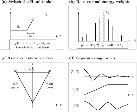
A quench calculation begins with the switch and the final-energy weights, then separates local observables, correlations, entanglement, and return probabilities. These diagnostics can have different front velocities, relaxation scales, and finite-size behavior.

The word “sudden” is always relative to specified dynamics. A ramp can be sudden for a slow collective mode and non-sudden for high-energy local excitations. Likewise, a spatially uniform parameter change can be experimentally inhomogeneous because of trapping, beam profiles, or calibration gradients.

Ideal Sudden Change

State continuity

Let the switch occupy the interval $-\tau_q/2<t<\tau_q/2$. Its exact propagator is

$$U_q = \mathcal T \exp\left[ -\frac{i}{\hbar} \int_{-\tau_q/2}^{\tau_q/2} H(t)\,dt \right].$$

In the ideal sudden limit, $U_q$ approaches the identity up to an irrelevant common phase on the relevant state support. Therefore

$$\rho(0^+)=\rho(0^-)=\rho_0.$$

The equality means that the density operator is the same abstract operator immediately before and after the switch. It does not mean that its energy probabilities are unchanged. The spectral projectors have changed from those of $H_i$ to those of $H_f$.

This continuity statement presupposes a common Hilbert space. If a geometry or ideal boundary quench changes operator domains or Hilbert-space realizations, one must specify an embedding or matching map before identifying the states at $0^-$ and $0^+$. The Sudden Approximation develops that domain caveat.

For an initial ket $|\psi_i\rangle$,

$$|\psi(0^+)\rangle = |\psi_i\rangle, \qquad |\psi(t)\rangle = e^{-iH_ft/\hbar} |\psi_i\rangle.$$

The ket is frozen during the ideal switch, then evolves with the final Hamiltonian.

A finite ramp is a different protocol

For nonzero $\tau_q$,

$$\rho(0^+) = U_q\rho(0^-)U_q^\dagger,$$

and transition amplitudes depend on the complete ramp shape. Merely writing $H_i\to H_f$ discards information needed to reproduce the state. The Sudden Approximation gives useful criteria such as the smallness of the integrated nontrivial generator on the occupied subspace.

There is no universal scalar threshold of the form “$\tau_q$ must be less than one second.” Relevant comparisons include

$$\tau_q \ll \frac{\hbar}{\Delta_{\mathrm{relevant}}},$$

where $\Delta_{\mathrm{relevant}}$ is a declared energy scale, and state-specific transition amplitudes generated during the ramp. Near a continuous quantum critical point, low-energy timescales diverge, so a ramp that is slow microscopically can still be nonadiabatic for critical modes. That critical-ramp problem is not identical to an ideal sudden quench.

A quench is not an impulse kick

An ideal parameter quench changes the generator and preserves the state across the switch:

$$H_i\longrightarrow H_f, \qquad \rho(0^+)=\rho(0^-).$$

An impulsive kick instead contributes a sharply localized Hamiltonian term whose time integral remains finite:

$$H(t) = H_0 + K\,\delta(t).$$

The kick produces the finite unitary

$$\begin{aligned} U_{\mathrm{kick}} &= e^{-iK/\hbar}, \\ \rho(0^+) &= U_{\mathrm{kick}} \rho(0^-) U_{\mathrm{kick}}^\dagger. \end{aligned}$$

The two operations have opposite idealized state-continuity rules and should not be conflated.

Taxonomy of Quenches

Global and local changes

Suppose a short-range lattice Hamiltonian is written as

$$H(\lambda) = \sum_X h_X(\lambda),$$

where $X$ labels bounded-diameter supports. A global quench changes an extensive set of terms. A homogeneous coupling quench,

$$\lambda_i\longrightarrow\lambda_f$$

at every site or bond, is the standard example. A local quench changes only $O(1)$ terms as the volume $V\to\infty$, such as:

• creating or removing one impurity;
• joining two chains at a bond;
• cutting one bond;
• changing a boundary field;
• adding one local potential.

The distinction concerns the support of $H_f-H_i$, not the spatial extent of the later wavefunction. A local quench can generate a disturbance that spreads through the entire system at late times.

Homogeneous and inhomogeneous changes

A global quench can be spatially uniform,

$$\lambda(\mathbf x,t>0)=\lambda_f,$$

or inhomogeneous,

$$\lambda(\mathbf x,t>0)=\lambda_f(\mathbf x).$$

Inhomogeneous protocols include domain-wall preparations, spatially varying fields, trap releases, expansion quenches, and joining reservoirs at different densities or temperatures. Translation invariance can no longer be assumed, and hydrodynamic profiles may be more informative than spatial averages.

State, interaction, field, and geometry quenches

Common labels describe what changes:

Quench type	Typical change	Immediate question
field quench	magnetic field or chemical potential	which final modes are populated?
interaction quench	interaction strength	how are correlations and quasiparticles generated?
hopping quench	tunneling amplitude or lattice depth	how do particles and correlations spread?
geometry quench	join, cut, release, or boundary change	how does a localized disturbance propagate?
disorder quench	random potential strength or realization	is transport suppressed or memory retained?
state quench	prepare a noneigenstate of a fixed $H$	how does the chosen state relax under that $H$?

A “state quench” is useful shorthand, but mathematically it is simply an unusual preparation followed by autonomous evolution. No Hamiltonian discontinuity is required at the chosen time origin.

Small and large quenches

A small parameter change $|\lambda_f-\lambda_i|\ll1$ does not by itself imply linear response. The relevant expansion can fail because:

• the initial and final ground states become orthogonal as $V\to\infty$;
• a gap closes;
• the perturbation acts for long times;
• the observable is singular in the thermodynamic limit;
• the change crosses a phase boundary.

Conversely, a large microscopic parameter change can produce simple dynamics when $H_f$ factorizes. “Small” should therefore identify the expansion parameter and the order of limits, not merely compare endpoint numbers.

The Post-Quench State in the Final Basis

Let the final Hamiltonian have spectral resolution

$$H_f = \sum_\alpha E_\alpha^f P_\alpha^f,$$

where $P_\alpha^f$ projects onto the full eigenspace of energy $E_\alpha^f$. Immediately after the ideal switch, the final-energy probabilities are

$$p_\alpha = \operatorname{Tr} \left( P_\alpha^f\rho_0 \right), \qquad \sum_\alpha p_\alpha=1.$$

For a pure state and nondegenerate spectrum,

$$\begin{aligned} |\psi_0\rangle &= \sum_n c_n|n_f\rangle, \\ c_n &= \langle n_f|\psi_0\rangle, \\ p_n &= |c_n|^2. \end{aligned}$$

The post-quench state is not a probabilistic mixture merely because it has many energy components. It is the coherent superposition

$$|\psi(t)\rangle = \sum_n c_n e^{-iE_n^ft/\hbar} |n_f\rangle.$$

Interference among these components drives time dependence.

Final energy and width

The first two final-energy moments are

$$\bar E_f = \operatorname{Tr}(\rho_0H_f),$$

and

$$(\Delta E_f)^2 = \operatorname{Tr}(\rho_0H_f^2) - \bar E_f^{\,2}.$$

These quantities answer different questions:

• $\bar E_f$ locates the energy density that a candidate equilibrium ensemble would need to reproduce;
• $\Delta E_f$ sets the short-time decay scale of the survival probability for a pure state;
• the full distribution $\{p_\alpha\}$ retains more information than either moment.

If $|\psi_0\rangle$ is an eigenstate of $H_i$ with energy $E_i$, the average energy injected by the ideal switch is

$$\Delta E_{\mathrm{inj}} = \langle\psi_0| (H_f-H_i) |\psi_0\rangle = \bar E_f-E_i.$$

This is an average energy change. Calling it “work” requires an operational convention; quantum work is not represented by a universal Hermitian operator. The Work Distributions page supplies that measurement ledger.

Excess energy above the final ground state

If $E_{0,f}$ is the final ground-state energy, define the excess energy

$$E_{\mathrm{exc}} = \bar E_f-E_{0,f} \ge 0.$$

For a volume $V$, the excess energy density is

$$e_{\mathrm{exc}} = \frac{E_{\mathrm{exc}}}{V}.$$

A nonzero $e_{\mathrm{exc}}$ generally places the state at finite energy density in the final spectrum. It does not identify a temperature until an equilibrium equation of state and the relevant conserved quantities are specified.

Scaling distinguishes global and local quenches

For bounded short-range terms and an initial eigenstate of $H_i$, or more generally a state whose pre-quench energy width is negligible compared with the quench-generated width:

$$\begin{aligned} \text{global mean shift} &=O(V), \\ \text{global final variance} &=O(V), \\ \text{local mean shift} &=O(1), \\ \text{local final variance} &=O(1). \end{aligned}$$

Thus a generic global quench from such a preparation has an extensive energy shift and a width $\Delta E_f=O(\sqrt V)$, while its relative energy-density width shrinks as $V^{-1/2}$. A local quench injects only finite total energy and adds only an $O(1)$ variance under the stated locality and clustering assumptions.

An initial Gibbs state already has an $O(V)$ energy variance in an ordinary thermodynamic regime. A local switch does not remove that pre-existing width. In that setting one should compare the change in moments or cumulants, rather than label the total final variance $O(1)$.

These scalings require qualifications. Critical long-range correlations, long-range interactions, unbounded local terms, or specially prepared macroscopic superpositions can change the variance. The assumptions should be stated rather than hidden behind the word “generic.”

Symmetry-sector audit

If a charge $Q$ commutes with $H_f$,

$$[H_f,Q]=0,$$

then the post-quench weights in its sectors are conserved. If the preparation lies in one sector,

$$Q|\psi_0\rangle=q|\psi_0\rangle,$$

the evolution never explores other sectors. Comparisons with random-matrix statistics, thermal ensembles, level spacings, or eigenstate expectation values must be performed within the same sector. Failing to resolve exact symmetries can manufacture apparent degeneracies and false nonthermal behavior.

Exact Evolution of Observables

For a Schrödinger-picture observable $O$ without explicit time dependence,

$$\langle O(t)\rangle = \operatorname{Tr} \left[ \rho_0 e^{iH_ft/\hbar} O e^{-iH_ft/\hbar} \right].$$

Equivalently, in the final energy basis,

$$\langle O(t)\rangle = \sum_{m,n} \rho_{mn}^{f} O_{nm}^{f} e^{-i(E_m^f-E_n^f)t/\hbar},$$

where

$$\begin{aligned} \rho_{mn}^{f} &= \langle m_f|\rho_0|n_f\rangle, \\ O_{nm}^{f} &= \langle n_f|O|m_f\rangle. \end{aligned}$$

This exact expression separates three ingredients:

1. preparation: the matrix elements $\rho_{mn}^{f}$;
2. spectrum: the final energy differences;
3. probe: the matrix elements $O_{nm}^{f}$.

No statement about relaxation follows from the spectrum alone.

When nothing happens

If

$$[H_f,\rho_0]=0,$$

then $\rho(t)=\rho_0$ and every time-independent observable is stationary. This can occur even when $H_i\ne H_f$. For example, if $H_i$ and $H_f$ share the prepared eigenstate, the parameter switch may change unoccupied energies without producing dynamics.

An individual observable is also constant whenever its expectation is protected, for example if

$$[H_f,O]=0.$$

Visible quench dynamics therefore requires both a nonstationary preparation and a probe coupled to the evolving coherences.

Short-time expansion

Expanding the Heisenberg operator gives

$$\begin{aligned} \langle O(t)\rangle ={}& \langle O\rangle_0 + \frac{it}{\hbar} \langle[H_f,O]\rangle_0 \\ & - \frac{t^2}{2\hbar^2} \langle[H_f,[H_f,O]]\rangle_0 + O(t^3). \end{aligned}$$

This provides an exact local audit:

• the first derivative vanishes if the first commutator has zero expectation;
• a flat initial slope does not imply a constant observable;
• nested commutators reveal how the support of a local operator grows.

For lattice Hamiltonians, each commutator can enlarge support only through terms overlapping the current support. This algebraic structure is the microscopic beginning of locality bounds.

Time averages and surviving coherence

The infinite-time average of the density operator, when it exists in the finite system, is

$$\overline{\rho} = \lim_{T\to\infty} \frac{1}{T} \int_0^T\rho(t)\,dt = \sum_\alpha P_\alpha^f \rho_0 P_\alpha^f.$$

Therefore

$$\overline{\langle O\rangle} = \operatorname{Tr} (\overline{\rho}\,O).$$

Coherences between distinct energies dephase in this average; coherences inside a degenerate eigenspace survive. Replacing the projectors $P_\alpha^f$ by arbitrary one-dimensional eigenvectors can incorrectly erase physical coherence.

The time-averaged state is often called the diagonal ensemble in a nondegenerate energy basis. It is fixed by all final-energy weights and is not automatically Gibbsian. Whether few-body observables agree with a thermal or generalized ensemble is the subject of the later thermalization pages.

Relaxation is observable-dependent

In a finite isolated system, $\langle O(t)\rangle$ is a quasiperiodic sum of phases and generally has recurrences. Operational equilibration means that a chosen observable stays close to a reference value for most times in a declared window, with fluctuations shrinking appropriately as size grows. One should report:

$$\delta O(t) = \langle O(t)\rangle - \overline{\langle O\rangle},$$

its temporal variance, system-size dependence, and the time interval used. A smooth curve from one finite size is evidence of dephasing, not a proof of asymptotic thermalization.

Correlations After a Quench

Connected changes isolate generated correlations

For local operators $A_x$ and $B_y$, define

$$\begin{aligned} C_{AB}^{\mathrm c}(x,y;t) ={}& \langle A_x(t)B_y(t)\rangle \\ &- \langle A_x(t)\rangle \langle B_y(t)\rangle. \end{aligned}$$

If the initial state already contains correlations, the quench-generated change

$$\begin{aligned} \Delta C_{AB}^{\mathrm c}(x,y;t) ={}& C_{AB}^{\mathrm c}(x,y;t) \\ &- C_{AB}^{\mathrm c}(x,y;0) \end{aligned}$$

is often more informative than the raw correlator. Otherwise an equilibrium background can be mistaken for propagation.

Unequal-time correlators,

$$\langle A_x(t)B_y(t')\rangle,$$

contain additional response and spectral information. Their full conventions belong to Time-Dependent Correlations.

Rigorous locality and observed fronts

For sufficiently local bounded lattice interactions, a Lieb–Robinson estimate has the schematic form

$$\begin{aligned} \left\| [A_X(t),B_Y] \right\| &\le C\, \|A_X\|\, \|B_Y\| \\ &\quad\times e^{-\mu[d(X,Y)-v_{\mathrm{LR}}|t|]}. \end{aligned}$$

Outside the effective cone $d(X,Y)\gtrsim v_{\mathrm{LR}}|t|$, influence is exponentially suppressed. The theorem does not imply:

• that every correlator has a sharp front;
• that the observed velocity equals $v_{\mathrm{LR}}$;
• that transport is ballistic;
• that long-range interactions obey the same linear cone;
• that correlations vanish exactly outside the cone.

Physical velocities can include quasiparticle group velocities, correlation velocities, sound velocities, diffusion scales, entanglement velocities, and butterfly velocities. They answer different questions.

The quasiparticle-pair picture

For many homogeneous global quenches in one-dimensional integrable systems, a useful semiclassical picture is:

1. the initial state acts as a spatially distributed source of entangled quasiparticle pairs;
2. partners with momenta $k$ and $-k$ move with velocities $v_k$ and $-v_k$;
3. two separated points become correlated when partners emitted from a common region can reach them.

For separation $r$, the fastest pair contribution arrives around

$$t_{\mathrm{front}} \sim \frac{r}{2v_{\max}}, \qquad v_{\max} = \max_k|v_k|.$$

The factor of two reflects partners moving in opposite directions. It should not be inserted blindly into operator-spreading or local-perturbation problems, where the geometry is different.

The pair picture is a controlled organizing principle in free and integrable settings and can remain qualitatively useful elsewhere. It is not a universal microscopic derivation for interacting chaotic systems. Scattering, diffusion, bound states, multiple species, confinement, or broad fronts may alter it.

Local quenches launch disturbances

A local change injects finite total energy near a region. The resulting density or correlation profile can contain:

• ballistic wavefronts carried by stable modes;
• dispersive broadening;
• diffusive conserved-density tails;
• bound-state oscillations near the defect;
• reflected and transmitted components at an interface.

Because the injected energy density vanishes as $V^{-1}$, a local quench does not generically prepare a spatially uniform finite-temperature state. Local observables far from the perturbation can remain near their original values until the disturbance arrives.

Entanglement Growth

Let the global post-quench state be pure and partition space into $A$ and its complement. The reduced state and von Neumann entropy are

$$\rho_A(t) = \operatorname{Tr}_{\bar A} |\psi(t)\rangle\langle\psi(t)|,$$ $$S_A(t) = -\operatorname{Tr} \left[ \rho_A(t)\ln\rho_A(t) \right].$$

Global unitarity preserves the entropy of the whole pure state, but interactions can redistribute quantum information so that $S_A(t)$ grows.

Integrable quasiparticle formula

For an interval of length $\ell$ in a one-dimensional integrable system, the pair picture motivates

$$\begin{aligned} S_A(t)-S_A(0) \simeq{}& \int\frac{dk}{2\pi}\, s(k) \\ &\times \min \left( 2|v_k|t,\ell \right). \end{aligned}$$

Here $s(k)$ is the entropy weight carried by quasiparticle pairs of momentum $k$, and $v_k$ is their group velocity. Equivalently,

$$\begin{aligned} S_A(t)-S_A(0) \simeq{}& 2t \int_{2|v_k|t<\ell} \frac{dk}{2\pi}\, |v_k|s(k) \\ & + \ell \int_{2|v_k|t>\ell} \frac{dk}{2\pi}\, s(k). \end{aligned}$$

The formula explains two broad features:

• early-time growth proportional to $t$, while entangled partners increasingly straddle the boundary;
• saturation proportional to $\ell$, once the finite interval is filled by contributing pairs.

Its assumptions matter. The entropy density and velocities depend on the initial state and final integrable model. Interacting nonintegrable systems can also exhibit linear entanglement growth, but not because a stable noninteracting pair formula is exact.

Entanglement growth is not energy transport

Entanglement can spread ballistically while a conserved energy density relaxes diffusively. Conversely, a free product evolution can change local observables and make the global Loschmidt echo exponentially small without generating any spatial entanglement.

One must therefore avoid a single generic “information velocity.” At minimum distinguish:

$$v_{\mathrm{LR}}, \qquad v_{\mathrm{corr}}, \qquad v_E, \qquad v_B,$$

for the locality bound, observed correlation front, entanglement growth, and operator front respectively. Equality can occur in special models but is not a definition.

Global and local quench scaling

A generic global quench from a short-range-entangled state can produce a late-time volume law for a finite region:

$$S_A(t\to\text{late}) \sim s_{\mathrm{ent}}V_A.$$

The coefficient need not equal the thermodynamic entropy density if the system is integrable, constrained, localized, or not yet equilibrated. The canonical distinctions live on Volume Laws.

A local joining quench in a one-dimensional critical system can instead generate logarithmic growth. In a conformal regime, a standard joining geometry gives schematically

$$S_A(t) \sim \frac{c}{3} \ln\left(\frac{t}{a}\right) + \text{constant},$$

within its scaling window, with central charge $c$ and short-distance cutoff $a$. This is not the generic law for every local quench.

Numerical consequence

Matrix-product-state methods represent low-entanglement states efficiently. If the bipartite entropy grows approximately linearly,

$$S(t)\sim s_E t,$$

then the required bond dimension often grows roughly as

$$\chi(t) \gtrsim e^{S(t)}.$$

Long-time real-time evolution can therefore become exponentially costly even in one dimension. Agreement at early times does not establish convergence at late times; bond dimension, truncation error, time step, and conserved quantities must be audited.

Loschmidt Amplitude and Return Probability

For a pure initial state, the Loschmidt amplitude under the final Hamiltonian is

$$\mathcal G(t) = \langle\psi_0| e^{-iH_ft/\hbar} |\psi_0\rangle.$$

The return probability, often called the Loschmidt echo in the quench literature, is

$$\mathcal L(t) = |\mathcal G(t)|^2.$$

In the final energy basis,

$$\mathcal G(t) = \sum_n p_n e^{-iE_n^ft/\hbar}.$$

Thus $\mathcal G(t)$ is the characteristic function of the post-quench energy distribution, up to the choice of sign and whether the Fourier variable has units of time or inverse energy. It is sensitive to the full distribution $\{p_n\}$.

Short-time decay

Expanding around $t=0$ gives

$$\begin{aligned} \mathcal G(t) ={}& 1 - \frac{i\bar E_f t}{\hbar} - \frac{\langle H_f^2\rangle_0t^2} {2\hbar^2} \\ & + O(t^3), \end{aligned}$$

and therefore

$$\mathcal L(t) = 1 - \frac{(\Delta E_f)^2t^2}{\hbar^2} + O(t^4).$$

The initial decay is quadratic, not exponential. Its scale is set by the final-energy uncertainty,

$$\tau_{\mathrm{surv}} \sim \frac{\hbar}{\Delta E_f}.$$

For a global quench with $(\Delta E_f)^2=O(V)$, this global overlap can decay on a size-dependent scale even while every local observable changes only modestly.

Intensive rate function

Because many-body overlaps often scale exponentially with volume, define

$$g(t) = -\lim_{V\to\infty} \frac{1}{V} \ln\mathcal L_V(t).$$

This intensive rate can remain finite when $\mathcal L_V(t)$ is exponentially small. In some models, $g(t)$ develops nonanalyticities at isolated critical times after the thermodynamic limit. These are called dynamical quantum phase transitions.

The qualification is essential:

• a small return probability is not itself a phase transition;
• a zero of a finite-size amplitude is not by itself thermodynamic criticality;
• nonanalyticity must be established by controlled size scaling;
• a return-rate singularity need not force a singularity in every local observable.

Loschmidt Echo and Dynamical Phase Transitions Preview owns the Fisher-zero construction, exact Ising-mode benchmark, finite-size evidence standards, and interpretation limits.

Terminology varies

In quantum-chaos and reversibility studies, “Loschmidt echo” often means sensitivity to imperfect reversal:

$$M(t) = \left| \langle\psi_0| e^{i(H_f+\delta H)t/\hbar} e^{-iH_ft/\hbar} |\psi_0\rangle \right|^2.$$

That quantity compares two evolutions. The quench return probability $\mathcal L(t)$ compares one evolved state with its initial state. A trustworthy paper or calculation writes the formula rather than relying on the shared name.

Mixed-state returns are not unique

For mixed $\rho_0$, one can form an interferometric amplitude

$$\mathcal G_{\mathrm{int}}(t) = \operatorname{Tr} \left[ \rho_0e^{-iH_ft/\hbar} \right],$$

but fidelity-based, purified, and interferometric return measures are inequivalent. No single mixed-state Loschmidt amplitude should be treated as automatic. The operational preparation and measurement protocol must choose the quantity.

Relation to Work Statistics

Suppose the system starts in a nondegenerate eigenstate $|i\rangle$ of $H_i$ with energy $E_i$, and final energy is measured after an ideal sudden switch. The two-projective-measurement distribution is

$$P(W) = \sum_n p_n\, \delta \left[ W-(E_n^f-E_i) \right],$$

where

$$p_n = |\langle n_f|i\rangle|^2.$$

With the convention

$$\chi(u) = \int dW\, e^{iuW} P(W),$$

one obtains

$$\begin{aligned} \chi(u) &= e^{-iuE_i} \sum_n p_n e^{iuE_n^f} \\ &= e^{-iuE_i} \mathcal G(-\hbar u). \end{aligned}$$

This relation is useful but conditional. Initial mixtures require the first energy measurement and its backaction to be included; coherent work definitions can differ. The quench energy distribution is a spectral property of $(\rho_0,H_f)$, whereas a work distribution is tied to a declared operational scheme.

Worked Example: Independent-Spin Global Quench

Consider $L$ spins prepared in

$$|\psi_0\rangle = |\uparrow_z\rangle^{\otimes L},$$

then evolved with

$$H_f = \frac{\hbar\Omega}{2} \sum_{j=1}^{L}\sigma_j^x.$$

All terms commute and the propagator factorizes:

$$U(t) = \bigotimes_{j=1}^{L} \exp \left( -\frac{i\Omega t}{2}\sigma_j^x \right).$$

For one spin,

$$\begin{aligned} |\psi_j(t)\rangle ={}& \cos\left(\frac{\Omega t}{2}\right) |\uparrow_z\rangle \\ &- i\sin\left(\frac{\Omega t}{2}\right) |\downarrow_z\rangle. \end{aligned}$$

Hence the longitudinal magnetization per site is

$$m_z(t) = \frac{1}{L} \sum_j \langle\sigma_j^z(t)\rangle = \cos(\Omega t).$$

The Loschmidt quantities are

$$\mathcal G(t) = \left[ \cos\left(\frac{\Omega t}{2}\right) \right]^L,$$ $$\mathcal L(t) = \left[ \cos^2\left(\frac{\Omega t}{2}\right) \right]^L,$$

and the finite-size rate per spin is

$$g_L(t) = -\frac{1}{L}\ln\mathcal L(t) = -2\ln \left| \cos\left(\frac{\Omega t}{2}\right) \right|.$$

The global return probability becomes exponentially small in $L$ at generic times, while $m_z(t)$ remains an order-one coherent oscillation. Moreover,

$$|\psi(t)\rangle = \bigotimes_j|\psi_j(t)\rangle$$

remains a product state, so every spatial bipartite entanglement entropy is zero. This exact counterexample demonstrates:

• overlap decay does not imply local relaxation;
• a global quench does not necessarily create entanglement;
• zeros of a finite-size return amplitude do not establish generic thermalization;
• an extensive final-energy variance can coexist with factorized dynamics.

Indeed,

$$\bar E_f=0, \qquad (\Delta E_f)^2 = L\left(\frac{\hbar\Omega}{2}\right)^2,$$

which reproduces the short-time echo expansion.

Worked Example: A Commuting Ising Entangler

Now prepare the $x$-polarized product state

$$|\psi_0\rangle = |+\rangle^{\otimes L}, \qquad \sigma^x|+\rangle=|+\rangle,$$

and quench to

$$H_f = J \sum_{j} \sigma_j^z\sigma_{j+1}^z.$$

All bond terms commute:

$$[ \sigma_j^z\sigma_{j+1}^z, \sigma_k^z\sigma_{k+1}^z ] = 0.$$

The evolution is a product of two-site phase gates,

$$U(t) = \prod_j \exp \left( -\frac{iJt}{\hbar} \sigma_j^z\sigma_{j+1}^z \right).$$

For a bulk site with two neighbors,

$$\langle\sigma_j^x(t)\rangle = \cos^2 \left( \frac{2Jt}{\hbar} \right).$$

Across a bipartition with a single bond crossing the cut, gates acting entirely within either side are local unitaries and do not change bipartite entropy. Only the crossing gate matters. Its two nonzero Schmidt probabilities are

$$\lambda_\pm(t) = \frac{1}{2} \left[ 1 \pm \left| \cos\left( \frac{2Jt}{\hbar} \right) \right| \right].$$

Therefore

$$S_{\mathrm{cut}}(t) = -\lambda_+\ln\lambda_+ -\lambda_-\ln\lambda_-.$$

At

$$\frac{2Jt}{\hbar} = \frac{\pi}{2} \pmod{\pi},$$

the cut entropy reaches $\ln2$. It later decreases because this integrable commuting model has exact revivals. The example separates interaction-generated entanglement from generic relaxation: the state entangles, but its dynamics remain highly structured and periodic.

Worked Example: Local Tight-Binding Release

Consider one particle initially localized at site $0$ on an infinite chain,

$$|\psi_0\rangle=|0\rangle,$$

with final Hamiltonian

$$H_f = -J \sum_{j\in\mathbb Z} \left( |j+1\rangle\langle j| + |j\rangle\langle j+1| \right).$$

The dispersion is

$$\varepsilon(k) = -2J\cos(ka),$$

and the group velocity is

$$v(k) = \frac{1}{\hbar} \frac{d\varepsilon}{dk} = \frac{2Ja}{\hbar}\sin(ka).$$

Thus

$$v_{\max} = \frac{2Ja}{\hbar}.$$

Fourier transformation gives the exact amplitude

$$\langle j|\psi(t)\rangle = i^j J_j \left( \frac{2Jt}{\hbar} \right),$$

where $J_j$ on the right is a Bessel function. The probability is

$$P_j(t) = J_j^2 \left( \frac{2Jt}{\hbar} \right).$$

Most weight lies inside the ballistic region

$$|j|a \lesssim v_{\max}t,$$

with a dispersive front rather than a perfectly sharp edge. This is coherent single-particle spreading, not diffusion and not many-body thermalization. It is nevertheless an exact model of how a local disturbance can fill an expanding spatial region.

A Practical Quench Workflow

Step 1: Define preparation and switch

Record:

$$\rho_0, \qquad H_i, \qquad H(t), \qquad H_f, \qquad \tau_q.$$

State whether $\rho_0$ is a ground state, eigenstate, Gibbs state, product state, domain wall, or experimentally reconstructed ensemble. Give boundary conditions, size, and symmetry sector.

Step 2: Compute conserved data

At minimum evaluate

$$\bar E_f, \qquad \Delta E_f, \qquad \langle Q_a\rangle_0$$

for every known exact conserved charge $Q_a$. If a proposed comparison ensemble violates these values, it is excluded before any fitting.

Step 3: Choose probes with distinct meanings

A useful set may include:

• one local observable;
• one conserved-density profile or current;
• one connected correlation function;
• one subsystem entropy or mutual information;
• one global return quantity.

Agreement among several probes is stronger than fitting one scalar. Disagreement is informative because different quantities can equilibrate on different timescales.

Step 4: Resolve time and length scales

Report the switching time, microscopic period, front-arrival time, relaxation window, boundary-reflection time, and recurrence scale when accessible. For a one-dimensional chain of length $L$ with characteristic front speed $v$, open boundaries contaminate central dynamics after a time of order

$$t_{\mathrm{refl}} \sim \frac{L}{2v},$$

up to preparation and probe geometry. Fits beyond that window need explicit finite-size modeling.

Step 5: Audit numerical convergence

For exact diagonalization:

• resolve every exact symmetry;
• compare several sizes and boundary conditions;
• separate infinite-time averages from finite-window averages;
• avoid interpreting recurrences as new phases.

For Krylov or product-formula evolution:

• reduce the time step or Krylov tolerance;
• monitor norm, energy, and exact charges;
• compare methods at representative times.

For matrix-product states:

• increase bond dimension;
• report discarded weight and entropy growth;
• compare one-site and two-site update conventions when relevant;
• stop claiming convergence when observables drift with $\chi$.

Step 6: Match experimental observables

Experiments implement finite ramps, imperfect initial states, spatial averaging, detection noise, and sometimes weak environmental coupling. Theory–experiment comparisons should use:

• the measured ramp profile;
• the actual trap or boundary conditions;
• the same coarse graining and observable estimator;
• uncertainty in calibrated couplings;
• independently measured decoherence and loss scales.

An ideal closed-system quench can be an excellent model without being a literal description of every experimental time.

Interpreting Common Outcomes

• Damped local oscillations support dephasing or relaxation of that observable; alone they do not establish Gibbs thermalization.
• Stationary local values support equilibration in the tested window; alone they do not establish loss of all memory.
• A ballistic correlation front supports finite-speed propagating correlations; alone it does not establish ballistic conserved transport.
• Linear entropy growth supports rapid entanglement production; alone it does not establish chaos or ETH.
• A small Loschmidt echo supports global state distinguishability; alone it does not establish local thermal behavior.
• Agreement with a Gibbs value supports consistency for selected probes; alone it does not establish uniqueness of the ensemble.
• Persistent oscillations support stable modes, constraints, or finite-size coherence; alone they do not establish integrability.
• A late-time volume law supports extensive subsystem entropy; alone it does not identify that entropy as thermal.

The page Nonequilibrium Overview gives the full vocabulary for dephasing, relaxation, equilibration, thermalization, stationarity, prethermalization, and recurrence.

Common Mistakes

• Treating a quench as a state collapse. An ideal Hamiltonian switch is unitary protocol control, not a measurement.
• Changing both Hamiltonian and state by hand. In the sudden limit, the state is continuous; its coordinates in the new energy basis change.
• Calling endpoint data a complete finite ramp. For $\tau_q>0$, the path and time ordering matter.
• Assuming every global quench heats to infinite temperature. Energy is conserved after the switch, and additional charges may constrain the state.
• Equating energy injection with temperature. Temperature requires an equilibrium relation and an appropriate ensemble.
• Dropping degeneracies in the time average. Coherences within equal-energy subspaces survive.
• Calling dephasing thermalization. Phase cancellation can yield stationary observables without Gibbs statistics.
• Reading one velocity from every front. Correlation, transport, entanglement, and operator fronts are different diagnostics.
• Using the quasiparticle-pair picture as a theorem for all systems. Its controlled domain is narrower than its intuitive usefulness.
• Inferring chaos from linear entanglement growth. Integrable systems can have linear growth.
• Inferring thermalization from a small return probability. Global overlap and local reduced states scale differently.
• Declaring a dynamical phase transition from a finite-size zero. Thermodynamic-limit scaling is essential.
• Ignoring the initial correlation background. Plot $\Delta C^{\mathrm c}$ when the state is already correlated.
• Comparing across symmetry sectors. The accessible final Hilbert space is fixed by conserved charges.
• Fitting after boundary reflections. The finite-size causal window must be identified first.
• Reporting only a visually smooth trace. Include errors, convergence, size scaling, and a comparison ensemble.

Exercises

1. State continuity and energy discontinuity

An initial pure state $|\psi_i\rangle$ is an eigenstate of $H_i$ with energy $E_i$. At $t=0$, the Hamiltonian is ideally quenched to $H_f$.

1. Show that the state is continuous at $t=0$.
2. Show that the mean energy can jump.
3. State a necessary and sufficient condition for the post-quench state to remain stationary.

Solution

In the ideal sudden limit, the propagator across the vanishing switch interval is the identity up to a common phase, so

$$|\psi(0^+)\rangle = |\psi(0^-)\rangle = |\psi_i\rangle.$$

The energy observable changes from $H_i$ to $H_f$. Therefore

$$\langle H\rangle_{0^-}=E_i, \qquad \langle H\rangle_{0^+} = \langle\psi_i|H_f|\psi_i\rangle,$$

and the mean jump is

$$\Delta E = \langle\psi_i| (H_f-H_i) |\psi_i\rangle.$$

The pure-state density operator remains stationary precisely when

$$[H_f,|\psi_i\rangle\langle\psi_i|]=0.$$

Equivalently, $|\psi_i\rangle$ lies entirely in one eigenspace of $H_f$. In a nondegenerate spectrum it must be a final energy eigenvector.

2. Spectral time average with degeneracy

Starting from

$$\rho(t) = e^{-iH_ft/\hbar}\rho_0e^{iH_ft/\hbar},$$

derive the infinite-time average in terms of the distinct-energy projectors $P_\alpha^f$. Explain why arbitrary basis dephasing inside a degenerate eigenspace is incorrect.

Solution

Insert

$$H_f = \sum_\alpha E_\alpha^fP_\alpha^f.$$

Then

$$\rho(t) = \sum_{\alpha,\beta} e^{-i(E_\alpha^f-E_\beta^f)t/\hbar} P_\alpha^f\rho_0P_\beta^f.$$

The long-time average of a phase vanishes for $E_\alpha^f\ne E_\beta^f$ and equals one for equal energies. Since $\alpha$ labels distinct energies,

$$\overline\rho = \sum_\alpha P_\alpha^f\rho_0P_\alpha^f.$$

Vectors within the same degenerate eigenspace acquire the same phase. Their mutual coherence is therefore time independent and cannot be removed by time averaging. A basis-dependent one-dimensional “diagonalization” would erase this physical coherence.

3. Independent-spin return rate

For the independent-spin quench above:

1. compute $(\Delta E_f)^2$;
2. expand $\mathcal L(t)$ through order $t^2$;
3. verify agreement with the universal short-time formula;
4. explain why $\mathcal L(t)\to0$ as $L\to\infty$ at generic fixed $t$ while the state remains unentangled.

Solution

Each spin has

$$\langle H_j\rangle_0=0, \qquad \langle H_j^2\rangle_0 = \left(\frac{\hbar\Omega}{2}\right)^2.$$

Cross covariances vanish in the product state, so

$$(\Delta E_f)^2 = L \left(\frac{\hbar\Omega}{2}\right)^2.$$

From

$$\mathcal L(t) = \left[ \cos^2\left(\frac{\Omega t}{2}\right) \right]^L,$$

and

$$\cos^2\left(\frac{\Omega t}{2}\right) = 1-\frac{\Omega^2t^2}{4}+O(t^4),$$

one obtains

$$\mathcal L(t) = 1-\frac{L\Omega^2t^2}{4}+O(t^4).$$

This equals

$$1-\frac{(\Delta E_f)^2t^2}{\hbar^2}+O(t^4).$$

At generic fixed $t$, the one-spin overlap magnitude is less than one, so its $L$th power vanishes exponentially. Yet the propagator factorizes into one-spin unitaries, which cannot create entanglement from the initial product state.

4. Entanglement from one Ising bond

Apply

$$U_\theta = e^{-i\theta\sigma_z\otimes\sigma_z}$$

to $|+\rangle|+\rangle$. Derive the reduced-state eigenvalues and identify when the pair is maximally entangled.

Solution

In the $z$ basis,

$$\begin{aligned} |\psi_\theta\rangle ={}& \frac{1}{2} \Bigl[ e^{-i\theta} (|00\rangle+|11\rangle) \\ &+ e^{i\theta} (|01\rangle+|10\rangle) \Bigr]. \end{aligned}$$

Tracing out the second spin gives

$$\rho_1 = \frac{1}{2} \begin{pmatrix} 1 & \cos(2\theta)\\ \cos(2\theta) & 1 \end{pmatrix}.$$

Its eigenvalues are

$$\lambda_\pm = \frac{1}{2} \left[ 1\pm|\cos(2\theta)| \right].$$

They are both $1/2$ when $\cos(2\theta)=0$, namely

$$\theta = \frac{\pi}{4} + \frac{n\pi}{2}.$$

The entropy is then $\ln2$.

5. Local versus global energy scaling

Let

$$H_f-H_i = \sum_{x\in R_V}\delta h_x,$$

where each $\|\delta h_x\|\le h_0$. Bound the magnitude of the mean injected energy when:

1. $|R_V|=O(V)$;
2. $|R_V|=O(1)$.

What extra assumption is needed to conclude that the variance is $O(V)$ in the first case?

Solution

The triangle inequality gives

$$\begin{aligned} \left| \operatorname{Tr} \left[ \rho_0(H_f-H_i) \right] \right| &\le \sum_{x\in R_V} \|\delta h_x\| \\ &\le h_0|R_V|. \end{aligned}$$

Thus the mean shift is at most $O(V)$ for a global quench and $O(1)$ for a local quench.

For the variance, write it as a sum of connected covariances of local terms. To obtain $O(V)$, one needs sufficient clustering or summability of those connected correlations. At a critical point, with long-range interactions, or in a macroscopic superposition, the covariance sum can scale faster.

6. Short-time Loschmidt law

For a normalized pure state and time-independent $H_f$, derive

$$\mathcal L(t) = 1-\frac{(\Delta E_f)^2t^2}{\hbar^2}+O(t^4).$$

Why is there no linear term?

Solution

The amplitude is

$$\mathcal G(t) = 1 - \frac{i\langle H_f\rangle t}{\hbar} - \frac{\langle H_f^2\rangle t^2}{2\hbar^2} + O(t^3).$$

Multiplying by its complex conjugate yields

$$|\mathcal G(t)|^2 = 1 - \frac{ \langle H_f^2\rangle - \langle H_f\rangle^2 }{\hbar^2} t^2 + O(t^4).$$

The linear phase cancels between $\mathcal G$ and $\mathcal G^*$. More generally,

$$\mathcal L(-t)=\mathcal L(t),$$

so the return probability is an even function of time whenever the expansion exists.

7. Single-speed quasiparticle model

Assume every entangled pair carries entropy weight density $s_0$ and moves with speed $v$. Use the pair formula to find the time dependence for an interval of length $\ell$.

Solution

If the momentum integral of the entropy weight is denoted by $s_0$, then

$$S_A(t)-S_A(0) = s_0 \min(2vt,\ell).$$

Therefore

$$S_A(t)-S_A(0) = \begin{cases} 2s_0vt, & t<\ell/(2v), \\ s_0\ell, & t>\ell/(2v). \end{cases}$$

The crossover time is the time required for opposite-moving partners to span the interval. Real dispersions smooth the kink because different modes have different velocities.

8. Design an evidence ledger

A simulation shows that one local density approaches the canonical-ensemble value after a global quench. List at least five additional checks needed before claiming thermalization.

Solution

A defensible ledger could include:

1. verify conservation of final energy and all known exact charges;
2. compare several system sizes within a pre-reflection time window;
3. test additional local observables and connected correlations;
4. compare temporal fluctuations with size;
5. resolve symmetry sectors;
6. compare with microcanonical as well as canonical predictions;
7. vary the initial state while holding energy density and charges fixed;
8. audit numerical time-step, truncation, and bond-dimension errors;
9. rule out a long-lived prethermal plateau;
10. report the order of the $V\to\infty$ and $t\to\infty$ limits.

Agreement of one observable is consistency evidence, not a mechanism.

References

1. A. Polkovnikov, K. Sengupta, A. Silva, and M. Vengalattore, “Colloquium: Nonequilibrium dynamics of closed interacting quantum systems,” Reviews of Modern Physics 83, 863–883 (2011). doi:10.1103/RevModPhys.83.863
2. P. Calabrese and J. Cardy, “Evolution of entanglement entropy in one-dimensional systems,” Journal of Statistical Mechanics: Theory and Experiment 2005, P04010 (2005). doi:10.1088/1742-5468/2005/04/P04010
3. P. Calabrese and J. Cardy, “Time dependence of correlation functions following a quantum quench,” Physical Review Letters 96, 136801 (2006). doi:10.1103/PhysRevLett.96.136801
4. M. A. Cazalilla, “Effect of suddenly turning on interactions in the Luttinger model,” Physical Review Letters 97, 156403 (2006). doi:10.1103/PhysRevLett.97.156403
5. P. Calabrese, F. H. L. Essler, and M. Fagotti, “Quantum quench in the transverse-field Ising chain,” Physical Review Letters 106, 227203 (2011). doi:10.1103/PhysRevLett.106.227203
6. A. M. Läuchli and C. Kollath, “Spreading of correlations and entanglement after a quench in the one-dimensional Bose–Hubbard model,” Journal of Statistical Mechanics: Theory and Experiment 2008, P05018 (2008). doi:10.1088/1742-5468/2008/05/P05018
7. S. Bravyi, M. B. Hastings, and F. Verstraete, “Lieb–Robinson bounds and the generation of correlations and topological quantum order,” Physical Review Letters 97, 050401 (2006). doi:10.1103/PhysRevLett.97.050401
8. J. Eisert and T. J. Osborne, “General entanglement scaling laws from time evolution,” Physical Review Letters 97, 150404 (2006). doi:10.1103/PhysRevLett.97.150404
9. M. Cheneau et al., “Light-cone-like spreading of correlations in a quantum many-body system,” Nature 481, 484–487 (2012). doi:10.1038/nature10748
10. S. Trotzky et al., “Probing the relaxation towards equilibrium in an isolated strongly correlated one-dimensional Bose gas,” Nature Physics 8, 325–330 (2012). doi:10.1038/nphys2232
11. T. Kinoshita, T. Wenger, and D. S. Weiss, “A quantum Newton’s cradle,” Nature 440, 900–903 (2006). doi:10.1038/nature04693
12. M. Rigol, V. Dunjko, and M. Olshanii, “Thermalization and its mechanism for generic isolated quantum systems,” Nature 452, 854–858 (2008). doi:10.1038/nature06838
13. M. Gring et al., “Relaxation and prethermalization in an isolated quantum system,” Science 337, 1318–1322 (2012). doi:10.1126/science.1224953
14. A. M. Kaufman et al., “Quantum thermalization through entanglement in an isolated many-body system,” Science 353, 794–800 (2016). doi:10.1126/science.aaf6725
15. A. Silva, “Statistics of the work done on a quantum critical system by quenching a control parameter,” Physical Review Letters 101, 120603 (2008). doi:10.1103/PhysRevLett.101.120603
16. M. Heyl, A. Polkovnikov, and S. Kehrein, “Dynamical quantum phase transitions in the transverse-field Ising model,” Physical Review Letters 110, 135704 (2013). doi:10.1103/PhysRevLett.110.135704
17. M. Heyl, “Dynamical quantum phase transitions: a review,” Reports on Progress in Physics 81, 054001 (2018). doi:10.1088/1361-6633/aaaf9a
18. H. Kim and D. A. Huse, “Ballistic spreading of entanglement in a diffusive nonintegrable system,” Physical Review Letters 111, 127205 (2013). doi:10.1103/PhysRevLett.111.127205
19. V. Alba and P. Calabrese, “Entanglement and thermodynamics after a quantum quench in integrable systems,” Proceedings of the National Academy of Sciences 114, 7947–7951 (2017). doi:10.1073/pnas.1703516114
20. U. Schollwöck, “The density-matrix renormalization group in the age of matrix product states,” Annals of Physics 326, 96–192 (2011). doi:10.1016/j.aop.2010.09.012
21. S. R. White and A. E. Feiguin, “Real-time evolution using the density matrix renormalization group,” Physical Review Letters 93, 076401 (2004). doi:10.1103/PhysRevLett.93.076401
22. A. J. Daley, C. Kollath, U. Schollwöck, and G. Vidal, “Time-dependent density-matrix renormalization-group using adaptive effective Hilbert spaces,” Journal of Statistical Mechanics: Theory and Experiment 2004, P04005 (2004). doi:10.1088/1742-5468/2004/04/P04005
23. L. D’Alessio, Y. Kafri, A. Polkovnikov, and M. Rigol, “From quantum chaos and eigenstate thermalization to statistical mechanics and thermodynamics,” Advances in Physics 65, 239–362 (2016). doi:10.1080/00018732.2016.1198134
24. L. Vidmar and M. Rigol, “Generalized Gibbs ensemble in integrable lattice models,” Journal of Statistical Mechanics: Theory and Experiment 2016, 064007 (2016). doi:10.1088/1742-5468/2016/06/064007

Further Connections

• Nonequilibrium Overview — the operational distinctions among dephasing, equilibration, and thermalization.
• Transverse-Field Ising Model — the standard exactly solvable global-quench benchmark.
• Bose–Hubbard Model — interaction quenches, Mott initial states, and experimentally observed correlation fronts.
• Time-Dependent Correlations — two-time functions, spectra, and nonequilibrium stationarity.
• Many-Body Entanglement Overview — subsystem, state-class, and measure conventions.
• Thermal Entropy versus Entanglement Entropy — why local thermal behavior is compatible with global purity.
• Operator Entanglement and Scrambling Preview — operator fronts and out-of-time-order diagnostics.
• Loschmidt Echo and Dynamical Phase Transitions Preview — Fisher zeros, thermodynamic return-rate singularities, and finite-size evidence.
• Thermodynamic Limit — the size limits behind rate functions and recurrences.
• Quenches — the quantum-matter bridge for switch waveforms, selective suddenness, excluded-band controls, platform observables, and pump–probe interpretation.

Summary

A quantum quench freezes the state during an ideal abrupt switch and then evolves that state under a new Hamiltonian. Its essential data are the preparation, final generator, switching protocol, probes, and limits.

The final-energy weights determine energy moments and the Loschmidt amplitude; final-energy coherences determine observable time dependence. Global and local quenches differ sharply in injected-energy scaling. Locality constrains spreading, but observed correlation, transport, entanglement, and operator velocities need not coincide.

Entanglement can grow without thermalization, local observables can oscillate while the global return probability vanishes exponentially with size, and finite systems can recur. Reliable conclusions therefore come from a ledger of conserved quantities, multiple diagnostics, finite-size and time-window controls, and numerical or experimental error analysis.