Entanglement and Criticality

Entanglement criticality is the use of subsystem entropies and related reduced-state data to identify, characterize, and test a quantum critical regime. In one spatial dimension, the ground-state entropy of an interval grows logarithmically at a conformal critical point, and the coefficient of that logarithm determines the conformal central charge. Away from criticality, a finite physical correlation length cuts off the growth. In numerical tensor-network states, finite bond dimension introduces another cutoff even when the exact state is critical.

The resulting method is powerful because it does not require a local order parameter. It is also easy to misuse. A trustworthy inference must distinguish:

• the physical correlation length $\xi(g)$ set by the Hamiltonian;
• the finite system size $L$;
• the subsystem size $\ell$ and its geometry;
• the finite-entanglement correlation length $\xi_\chi$ of an approximate state;
• ultraviolet and boundary corrections;
• and genuine ground-state entanglement from thermal or classical mixed-state entropy.

The slogan “entropy is logarithmic at criticality” is only the beginning. The geometry-dependent coefficient, the finite-size chord, the scaling window, and the competing infrared cutoffs carry the quantitative content.

Canonical Scope

This page owns the inference problem: how entanglement data are used to test one-dimensional criticality, extract a central charge, locate a transition, and separate finite-size from finite-entanglement scaling.

Neighboring pages retain the canonical treatments of the ingredients:

• Entanglement Entropy in Many-Body Systems defines spatial von Neumann and Rényi entropies and surveys their scaling across state classes.
• Quantum Phase Transitions defines phases and transitions and explains why finite systems remain smooth.
• Critical Exponents and Scaling owns the general finite-size-scaling formalism, correction fields, pseudocritical drift, and data-collapse statistics.
• Matrix Product States Preview owns MPS tensors, canonical gauges, Schmidt truncation, and transfer operators.
• Entanglement Spectrum owns level-resolved reduced-state structure and boundary-CFT tower interpretations.
• Luttinger Liquid Preview owns the compact-boson theory, the Luttinger parameter, and the operator exponents along a common $c=1$ critical line.

The conformal formulas needed for inference are stated here with their domains of validity. A full derivation of conformal field theory, twist fields, and operator content belongs to the field-theory volumes.

Setup and Convention Ledger

Consider a one-dimensional Hamiltonian $H(g)$ depending on a control parameter $g$. Unless stated otherwise, assume:

• a pure ground state $\lvert\psi(g,L)\rangle$;
• a lattice spacing or short-distance regulator $a$;
• a contiguous interval $A$ of length $\ell$;
• natural logarithms, so entropy is measured in nats;
• a clean, short-range system whose critical point has a unitary relativistic continuum limit;
• and a nonchiral $1+1$-dimensional conformal field theory with central charge $c$.

The reduced state and its Rényi entropies are

$$\begin{aligned} \rho_A &= \operatorname{Tr}_{\bar A} \lvert\psi\rangle\langle\psi\rvert, \\ S_n(A) &= \frac{1}{1-n} \ln\operatorname{Tr}\rho_A^n, \qquad n>0, \end{aligned}$$

with von Neumann limit

$$S(A) = \lim_{n\to1}S_n(A) = -\operatorname{Tr}\rho_A\ln\rho_A.$$

Three lengths must not be conflated:

$$\begin{aligned} \xi(g) &: \text{physical}, \\ L &: \text{finite size}, \\ \xi_\chi &: \text{finite entanglement}. \end{aligned}$$

At an exact continuous critical point, $\xi(g_c)=\infty$. A finite calculation still has an infrared cutoff supplied by $L$, $\xi_\chi$, temperature, or another perturbation. The smallest relevant scale usually controls the first crossover, but replacing all crossover functions by a literal minimum is only a mnemonic.

Why Criticality Changes Spatial Entanglement

For a generic one-dimensional gapped ground state of a local Hamiltonian, correlations decay over a finite length and the interval entropy approaches a constant once both $\ell$ and its complement are large compared with $\xi$. This is the one-dimensional area-law pattern: the boundary of a connected interval consists of a fixed number of points.

At a scale-invariant critical point, degrees of freedom remain correlated on every scale between the regulator and the infrared cutoff. Each logarithmic band of length scales contributes a comparable amount to the entanglement across the cut. Summing those contributions gives

$$S_A \propto \ln\frac{\text{infrared scale}}{a}.$$

This picture explains the logarithm but not its universal coefficient. Conformal symmetry fixes that coefficient in terms of $c$ and the number and geometry of entangling points.

The implication is one-way unless supporting assumptions are established:

A clean one-dimensional ground state governed by a unitary $1+1$-dimensional CFT has a specific logarithmic entropy law. Observing an approximate logarithm over a short range does not by itself prove conformal criticality.

Logarithms can also arise from Fermi surfaces, disorder-controlled fixed points, corners in higher dimensions, mixtures, crossovers, or fitting artifacts.

Replica and Twist-Field Preview

The Rényi entropy is convenient because integer moments $\operatorname{Tr}\rho_A^n$ can be represented by $n$ replicated copies sewn cyclically along $A$. For one interval on an infinite line, the endpoints act as branch points. In a conformal description they are represented by twist fields with total scaling dimension

$$\Delta_n = \frac{c}{12} \left( n-\frac1n \right).$$

Their two-point function gives

$$\operatorname{Tr}\rho_A^n = C_n \left( \frac{\ell}{a} \right)^{-2\Delta_n},$$

where $C_n$ is nonuniversal. Substitution into the Rényi definition yields

$$S_n(\ell) = \frac{c}{6} \left( 1+\frac1n \right) \ln\frac{\ell}{a} +s_n.$$

The additive constant

$$s_n = \frac{ \ln C_n }{1-n}$$

depends on the microscopic regulator and normalization. It is not a universal observable. The coefficient of the logarithm is universal within the stated geometry and universality class.

Taking $n\to1$ gives

$$S(\ell) = \frac{c}{3} \ln\frac{\ell}{a} +s_1.$$

The interval has two entangling points. A half-infinite bipartition or a block attached to a physical boundary has one, which is the origin of several factors of two below.

Finite Periodic Chains and the Chord Length

For a periodic chain of circumference $L$, the conformal map from the plane to the cylinder replaces the interval length by the chord length

$$d_L(\ell) = \frac{L}{\pi} \sin\left( \frac{\pi\ell}{L} \right).$$

The finite-size Rényi formula is

$$\begin{aligned} S_n(\ell,L) &= \frac{c}{6} \left( 1+\frac1n \right) \ln\left[ \frac{d_L(\ell)}{a} \right] \\ &\quad {} +s_n +\delta S_n. \end{aligned}$$

Here $\delta S_n$ collects finite-size, lattice, irrelevant-operator, and numerical corrections. For the von Neumann entropy,

$$\begin{aligned} S(\ell,L) &= \frac{c}{3} \ln\left[ \frac{d_L(\ell)}{a} \right] \\ &\quad {} +s_1 +\delta S_1. \end{aligned}$$

The formula automatically satisfies the pure-state symmetry

$$S_n(\ell,L) = S_n(L-\ell,L).$$

At half chain,

$$\begin{aligned} S_n(L/2,L) &= \frac{c}{6} \left( 1+\frac1n \right) \ln\frac{L}{\pi a} \\ &\quad {} +s_n +\delta S_n. \end{aligned}$$

Fitting $S$ directly against $\ln\ell$ across an appreciable fraction of a finite ring bends a known geometric effect into the inferred slope. The chord length is not an optional correction; it is the leading conformal prediction for that geometry.

Open Chains and Boundary Entropy

For an open chain of length $L$, let $A$ be the interval from one physical end to a cut at $\ell$. There is one entangling point. Define the open-chain chord

$$d_L^{\mathrm{open}}(\ell) = \frac{2L}{\pi} \sin\left( \frac{\pi\ell}{L} \right).$$

For conformal boundary conditions,

$$\begin{aligned} S_n^{\mathrm{open}}(\ell,L) &= \frac{c}{12} \left( 1+\frac1n \right) \ln\left[ \frac{d_L^{\mathrm{open}}(\ell)}{a} \right] \\ &\quad {} +b_n +\ln g_{\mathrm B} +\delta S_n^{\mathrm{open}}. \end{aligned}$$

The constant $b_n$ depends on microscopic conventions. The quantity $\ln g_{\mathrm B}$ is the Affleck–Ludwig boundary entropy for the boundary condition encountered by the conformal problem. Extracting it requires matching regulator-dependent constants or comparing controlled boundary conditions; it cannot be read reliably from one unconstrained intercept.

For $n=1$, the leading logarithmic coefficient is $c/6$, half the periodic-interval coefficient $c/3$. This factor reflects one entangling point rather than two.

The formula above is specifically for a block attached to a physical end. An interval floating inside an open chain has a different boundary-CFT geometry and generally involves more than the simple one-point expression. Choosing the wrong formula can produce a numerically plausible but physically meaningless “central charge.”

Gapped Crossover Near a Critical Point

Suppose $g$ approaches a continuous critical point from a gapped phase and

$$\xi(g) \sim \xi_0 \lvert g-g_c\rvert^{-\nu}.$$

For an interval much larger than $\xi$ in an infinite system, the entropy saturates. Near a relativistic conformal critical point, its singular part scales as

$$\begin{aligned} S_n^{\mathrm{sat}} &= \mathcal A \frac{c}{12} \left( 1+\frac1n \right) \ln\frac{\xi}{a} \\ &\quad {} +\text{constant} +\cdots, \end{aligned}$$

where $\mathcal A$ is the number of entangling points. For the von Neumann entropy,

$$S^{\mathrm{sat}} = \mathcal A \frac{c}{6} \ln\frac{\xi}{a} +\text{constant} +\cdots.$$

Thus an interval in an infinite line has $\mathcal A=2$ and leading coefficient $c/3$, while a half-infinite cut has $\mathcal A=1$ and coefficient $c/6$.

The frequently written interpolation

$$S \sim \frac{c}{3} \ln\frac{\min\{\ell,\xi\}}{a}$$

captures the limiting scales for a two-ended interval, but it is not the universal crossover function. Quantitative fits should use an appropriate scaling ansatz rather than differentiate or optimize this mnemonic.

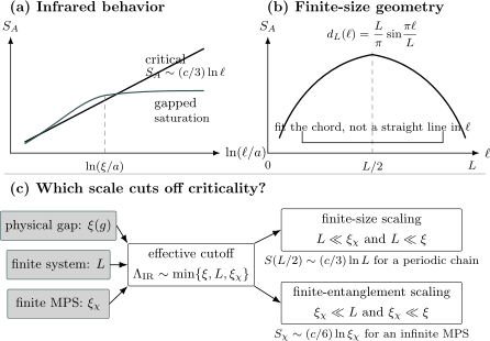
Entanglement scaling is an infrared ledger. A gapped state saturates when $\ell$ exceeds $\xi$, whereas a conformal critical state grows logarithmically. A finite ring replaces $\ell$ by its chord $d_L(\ell)$. In numerical work, the relevant regime depends on the ordering of $\xi(g)$, $L$, and the MPS correlation length $\xi_\chi$.

What the Central Charge Does and Does Not Identify

In a two-dimensional conformal field theory, the central charge appears in the Virasoro algebra, the trace anomaly, the finite-size ground-state energy, and the interval-entanglement coefficient. It is a universal property of the fixed point.

Operationally, $c$ measures aspects of the low-energy degrees of freedom, but it is not simply a count of microscopic particles or lattice fields. Standard examples include:

$$\begin{array}{c|c} \text{critical theory} & c \\ \hline \text{Ising CFT} & 1/2 \\ \text{tricritical Ising CFT} & 7/10 \\ \text{compact free boson} & 1 \\ \text{two independent Ising theories} & 1 \end{array}$$

The last two entries illustrate an essential limitation: $c$ alone does not determine the operator content, compactification radius, symmetries, boundary conditions, or universality class. Along a Luttinger-liquid fixed line, $c=1$ remains fixed while the Luttinger parameter and correlation exponents vary continuously.

A central-charge estimate is therefore a consistency test and classifier, not a complete identification. It should be combined with spectra, correlations, symmetry sectors, scaling dimensions, and phase diagnostics.

Extracting the Central Charge

Profile fit on a periodic ring

Define

$$x_\ell = \ln d_L(\ell).$$

Ignoring the cutoff inside the intercept, the leading fit is

$$S_n(\ell,L) = \alpha_n x_\ell +\beta_n +\delta S_n(\ell,L),$$

with

$$\alpha_n = \frac{c}{6} \left( 1+\frac1n \right).$$

Hence

$$c = \frac{6\alpha_n}{1+1/n}.$$

For $n=1$,

$$c = 3\alpha_1.$$

A fit should exclude intervals comparable to $a$, include the covariance of entropies computed from the same state, and be repeated over several minimum-block and maximum-block windows. A small least-squares residual does not validate the CFT model if the window contains too few distinct scales.

Difference estimator

Taking a difference removes the nonuniversal constant. For two intervals on the same periodic chain,

$$\begin{aligned} c_{\mathrm{eff}}^{(n)} (\ell_1,\ell_2;L) &= \frac{6}{1+1/n} \\ &\quad {} \times \frac{ S_n(\ell_2,L)-S_n(\ell_1,L) }{ \ln[d_L(\ell_2)/d_L(\ell_1)] }. \end{aligned}$$

For the von Neumann entropy,

$$c_{\mathrm{eff}} = 3 \frac{ S(\ell_2,L)-S(\ell_1,L) }{ \ln[d_L(\ell_2)/d_L(\ell_1)] }.$$

This estimator is useful for visualization, but it is not automatically more accurate than a global fit. Differences amplify numerical noise, and nearby points can make the denominator small. A plateau under changing pairs and sizes is more meaningful than one favorable value.

Half-chain differences across sizes

For periodic chains with the same microscopic model and boundary sector, define

$$\begin{aligned} \Delta_L S_n &\equiv S_n(L_2/2,L_2) \\ &\quad {} -S_n(L_1/2,L_1). \end{aligned}$$

Then

$$c_{\mathrm{eff}}^{(n)}(L_1,L_2) = \frac{6}{1+1/n} \frac{\Delta_L S_n}{\ln(L_2/L_1)}.$$

For $n=1$ this becomes

$$c_{\mathrm{eff}}(L_1,L_2) = 3 \frac{\Delta_L S_1}{\ln(L_2/L_1)}.$$

For a half-chain cut in open systems, define

$$\begin{aligned} \Delta_L S_n^{\mathrm{open}} &\equiv S_n^{\mathrm{open}}(L_2/2,L_2) \\ &\quad {} -S_n^{\mathrm{open}}(L_1/2,L_1). \end{aligned}$$

The leading coefficient is half as large, so

$$\begin{aligned} c_{\mathrm{eff,open}}^{(n)} &= \frac{12}{1+1/n} \\ &\quad {} \times \frac{\Delta_L S_n^{\mathrm{open}}}{\ln(L_2/L_1)}. \end{aligned}$$

The boundary conditions and ground-state sector must match between sizes. Otherwise boundary entropies, edge modes, parity changes, or sector crossings need not cancel.

Rényi consistency

The leading conformal slope predicts the full $n$ dependence

$$\frac{\alpha_n}{\alpha_1} = \frac12 \left( 1+\frac1n \right).$$

Agreement of several Rényi orders with a common $c$ is stronger evidence than agreement of one entropy. It is not an exact finite-size requirement: branch-point corrections often depend strongly on $n$, and large-$n$ entropies are especially sensitive to the largest Schmidt values and truncation errors.

Locating a Critical Point with Entanglement

Let $g$ tune a Hamiltonian through a candidate critical point. Several entanglement-based pseudocritical estimators are common:

• the location of a maximum in the half-chain entropy;
• the location at which an interval profile best fits the conformal chord formula;
• the location of a peak or crossing in an effective central charge;
• the location at which $S$ versus $\ln\xi_\chi$ is most nearly linear;
• or the location of a feature in an entanglement-spectrum gap.

Each estimator is finite-size, finite-bond, and definition dependent. Write its result as

$$g^*(L,\chi,\mathcal B),$$

where $\mathcal B$ records boundary conditions, symmetry sector, subsystem convention, and estimator. The thermodynamic critical coupling is inferred only after controlled limits.

A local maximum of entropy is neither necessary nor sufficient for a continuous transition. It can be shifted by boundaries, occur inside a gapless phase, be rounded by a finite bond dimension, or arise at an avoided crossing. Conversely, symmetry constraints or competing corrections can make the expected maximum too broad to resolve.

The defensible claim is comparative:

A candidate $g_c$ is supported when several sizes and bond dimensions approach a common point, the entropy profile has the geometry-correct conformal form there, the inferred $c$ stabilizes, and independent spectral or correlation diagnostics agree.

Finite-Size Scaling of the Entropy

For an ordinary continuous transition with one relevant tuning field

$$u(g) = u_1(g-g_c) +u_2(g-g_c)^2 +\cdots,$$

the physical correlation length scales as

$$\xi(g) \sim \lvert u\rvert^{-\nu}.$$

At a periodic half-chain cut and sufficiently large bond dimension, a useful finite-size ansatz is

$$\begin{aligned} S_n(g,L) &= \frac{c}{6} \left( 1+\frac1n \right) \ln\frac{L}{a} \\ &\quad {} +\mathcal F_n \left( uL^{1/\nu} \right) +\delta S_n(g,L). \end{aligned}$$

The constant $-\alpha_n\ln\pi$ has been absorbed into $\mathcal F_n$. A convenient subtracted observable is

$$\widetilde S_n(g,L;c) = S_n(g,L) - \frac{c}{6} \left( 1+\frac1n \right) \ln L.$$

If the assumed $g_c$, $c$, $\nu$, and correction model are appropriate, data at different $L$ can collapse when plotted against $uL^{1/\nu}$. Such a collapse is conditional evidence, not a visual proof. The same data determine several fitted parameters and are strongly correlated across nearby $g$ and $L$.

For an estimator whose extremum tracks a fixed scaling argument,

$$g^*(L)-g_c \sim L^{-1/\nu}$$

at leading order. Irrelevant fields and nonlinear scaling variables modify this drift:

$$g^*(L)-g_c = A L^{-1/\nu} \left( 1+B L^{-\omega}+\cdots \right).$$

This power law is not universal across all transition types. The Critical Exponents and Scaling page gives the canonical treatment of drift, correction exponents, covariance, and model comparison.

Entropy derivatives

Differentiating the scaling ansatz suggests

$$\left. \frac{\partial S_n}{\partial g} \right|_{g_c} \sim L^{1/\nu} \mathcal F_n'(0)$$

when the leading derivative does not vanish. In practice, numerical differentiation amplifies state-optimization error, interpolation error, and parameter-grid noise. A derivative peak should be fitted jointly with its width and drift and checked against direct profile fits.

The derivative can also be constrained by symmetries. If $S_n(g,L)$ is locally even in the relevant scaling field, then $\mathcal F_n'(0)=0$ and the leading derivative test fails despite genuine criticality.

Transitions That Need Different Logic

First-order transitions

At a first-order quantum transition, finite systems often show an avoided crossing. A symmetric finite-volume ground state can become a superposition of macroscopically distinct states, adding an approximately constant “cat-state” contribution such as $\ln2$. This can create an entropy peak without a conformal logarithm.

Evidence for first-order behavior should instead examine level crossings or exponentially small avoided gaps, discontinuous observables, phase coexistence, and size scaling appropriate to the boundary conditions. Fitting a central charge to a few sizes near a crossing can return a number even when no critical CFT exists.

Berezinskii–Kosterlitz–Thouless transitions

At a Berezinskii–Kosterlitz–Thouless transition, the correlation length has an essential singularity,

$$\xi \sim \xi_0 \exp\left( \frac{b}{\sqrt{\lvert g-g_c\rvert}} \right),$$

rather than a finite power-law exponent $\nu$. A common pseudocritical drift is therefore logarithmic,

$$g^*(L)-g_c \sim \frac{1}{(\ln L+B)^2},$$

up to model- and estimator-dependent corrections. Treating the drift as $L^{-1/\nu}$ can produce a stable but fictitious effective exponent over modest sizes.

Berezinskii–Kosterlitz–Thouless points also suffer from marginal logarithmic corrections. Entanglement can still support $c=1$ criticality, but locating the endpoint usually requires level spectroscopy, Luttinger-parameter criteria, stiffness, or other model-specific information.

Extended gapless phases

In a Luttinger liquid, an entire interval of couplings can have $c=1$. The entropy therefore identifies a gapless phase rather than a unique critical point. The changing physics along the line is encoded in the Luttinger parameter and scaling dimensions, not in $c$.

A broad $c\approx1$ plateau is expected evidence in this setting. Selecting its largest entropy as “the” transition point discards the fixed-line structure.

Disorder and nonstandard fixed points

At random critical points, disorder-averaged entropies can have logarithmic coefficients described by an effective central charge that is not the ordinary central charge of a clean unitary CFT. Long-range interactions, nonrelativistic fixed points with $z\ne1$, nonunitary theories, and Lifshitz points can also modify the standard formulas.

The assumptions behind the conformal estimator must therefore be tested before interpreting its slope as $c$.

Finite-Entanglement Scaling

An infinite uniform MPS with finite bond dimension $\chi$ has a transfer operator with a discrete spectrum. If its two leading eigenvalues in magnitude are $\mu_1$ and $\mu_2$, normalized so $\lvert\mu_1\rvert=1$, then

$$\xi_\chi = -\frac{1}{ \ln\lvert\mu_2/\mu_1\rvert }.$$

For a generic injective finite-$\chi$ MPS, connected correlations are asymptotically exponential. It therefore cannot exactly reproduce an infinite critical state with algebraic correlations. Variational optimization responds by making $\xi_\chi$ grow with $\chi$.

At a one-dimensional conformal critical point, the half-chain entropy obeys the finite-entanglement relation

$$S_\chi = \frac{c}{6} \ln\frac{\xi_\chi}{a} +s_\chi +\delta S_\chi.$$

The factor $c/6$ corresponds to one entangling cut. This equation is one of the most useful numerical central-charge estimators because it uses the measured infrared scale $\xi_\chi$ rather than assuming how that scale depends on $\chi$.

For two well-converged bond dimensions,

$$c_{\mathrm{eff}} = 6 \frac{ S_{\chi_2}-S_{\chi_1} }{ \ln(\xi_{\chi_2}/\xi_{\chi_1}) }.$$

A global fit of $S_\chi$ against $\ln\xi_\chi$ is preferable to a single pair. One should vary the smallest retained $\chi$, verify transfer-spectrum convergence, and check more than one MPS unit cell or symmetry implementation.

Bond-dimension exponent

For optimized MPS approximations in the asymptotic conformal regime,

$$\xi_\chi \propto \chi^\kappa.$$

Finite-entanglement theory predicts

$$\kappa(c) = \frac{6}{ c\left( \sqrt{12/c}+1 \right) }.$$

Combining this result with $S_\chi=(c/6)\ln\xi_\chi+\cdots$ gives

$$S_\chi = \frac{c\kappa}{6} \ln\chi +\text{constant} +\cdots,$$

or equivalently

$$\frac{c\kappa}{6} = \frac{1}{ \sqrt{12/c}+1 }.$$

These expressions are asymptotic predictions based on the conformal reduced-density-matrix spectrum and an optimized finite-entanglement approximation. They are not kinematic identities for every arbitrary MPS of bond dimension $\chi$. Preasymptotic behavior depends on algorithm, unit cell, symmetry constraints, initialization, and the operator content that controls corrections.

Consequently, fitting $S$ directly against $\ln\chi$ is less assumption-light than fitting $S$ against the measured $\ln\xi_\chi$.

Finite-size versus finite-entanglement regimes

At the exact critical coupling, a finite periodic MPS calculation depends on the ratio

$$y = \frac{L}{\xi_\chi}.$$

For the half-chain Rényi entropy, a crossover form is

$$\begin{aligned} S_n(L,\chi) &= \alpha_n\ln L +\Phi_n \left( \frac{L}{\xi_\chi} \right) +\cdots, \\ \alpha_n &= \frac{c}{6} \left( 1+\frac1n \right). \end{aligned}$$

The limiting regimes are:

• Finite-size regime: if $L\ll\xi_\chi$, then $S_n\sim\alpha_n\ln L$.
• Finite-entanglement regime: if $\xi_\chi\ll L$, then $S_n\sim\alpha_n\ln\xi_\chi$.

In the second limit, the crossover function must behave schematically as

$$\Phi_n(y) \sim -\alpha_n\ln y +\text{constant}, \qquad y\gg1,$$

so that the explicit $\ln L$ cancels and the entropy saturates at the finite-entanglement scale.

Off criticality, the physical correlation length supplies a third ratio. A general scaling description may be organized as

$$\begin{aligned} S_n(g,L,\chi) &= \alpha_n\ln L \\ &\quad {} +\Phi_n\left( \frac{L}{\xi(g)}, \frac{L}{\xi_\chi} \right) +\cdots. \end{aligned}$$

The two arguments distinguish:

• physical saturation, $\xi(g)\ll L,\xi_\chi$;
• finite-size scaling, $L\ll\xi(g),\xi_\chi$;
• finite-entanglement scaling, $\xi_\chi\ll L,\xi(g)$;
• and crossover regions where no single one-variable fit is adequate.

Scaling other observables with the MPS correlation length

If an observable $O$ has critical scaling dimension $x_O$, finite-entanglement scaling suggests

$$O(g,\chi) = \xi_\chi^{-x_O} \mathcal G_O \left( u\xi_\chi^{1/\nu} \right) +\cdots.$$

At $g=g_c$,

$$O(g_c,\chi) \propto \xi_\chi^{-x_O}.$$

This provides an independent check: the same $\xi_\chi$ that organizes the entropy should organize order parameters, gaps, and correlations with mutually consistent scaling dimensions. An entropy-only fit leaves more room for accidental agreement.

Correction Ledger

The leading conformal expression should be treated as the first term of a controlled asymptotic model. A practical periodic-chain fit may take the form

$$\begin{aligned} S_n(\ell,L) &= \alpha_n \ln\frac{d_L(\ell)}{a} +s_n \\ &\quad {} +A_n \frac{ \cos(2k_F\ell+\varphi_n) }{ [d_L(\ell)/a]^{p_n} } \\ &\quad {} +B_n [d_L(\ell)/a]^{-\omega_n} +\cdots. \end{aligned}$$

This is a modeling template, not a universal formula with arbitrary free exponents. The allowed oscillations and correction powers should be motivated by symmetry, filling, boundary condition, and low-energy operator content.

Ultraviolet points

Blocks with $\ell$ only a few lattice spacings long do not lie in the continuum regime. The complementary endpoint $L-\ell$ has the same problem. Removing these points is not cherry-picking if the exclusion rule is stated before fitting and stability is shown as the cutoff changes.

Irrelevant operators

Irrelevant bulk and boundary operators produce algebraic corrections. Their powers can differ from those in ordinary thermodynamic observables because Rényi replicas contain conical branch points. For some $n$, branch-point operators generate “unusual” correction exponents that dominate the naive irrelevant-field term.

This is why forcing every Rényi order to share one correction power can bias the common central charge even when their leading slopes are correct.

Marginally irrelevant operators

Marginally irrelevant couplings generate slow logarithmic drift. The isotropic antiferromagnetic Heisenberg chain is a standard example. A fitted $c_{\mathrm{eff}}(L)$ can approach $1$ so slowly that a constant-plus-power correction looks convincing over accessible sizes.

One should compare logarithmic and power-correction models, use model-specific field-theory information when available, and report the remaining extrapolation uncertainty.

Parity and Friedel oscillations

Open boundaries break translation symmetry and can induce alternating bond energies and entanglement entropies. In critical XXZ chains, even and odd cuts can form visibly distinct branches. Averaging them blindly can create a curved profile and a biased slope.

Defensible options include:

• fitting parity sectors separately with a common leading $c$;
• including an oscillatory correction with a theoretically motivated wavevector;
• or restricting to a symmetry-related subsequence and reporting that choice.

Sector and degeneracy effects

Changing system size can change the lowest-energy momentum, parity, particle-number sector, or edge-state occupation. A nearly degenerate finite-size manifold can contribute constants or discontinuities unrelated to the bulk central charge.

The state-selection rule must be fixed across sizes. If a symmetry-broken branch and a symmetric cat state are both studied, their entropy difference should be interpreted as sector structure rather than as a changed critical coefficient.

Numerical optimization error

Entropy is often more sensitive to small Schmidt values than the energy. A state can have a highly converged energy while its Rényi entropies, correlation length, and entanglement spectrum still drift with $\chi$.

For each data point, monitor at least:

• energy variance or another stationarity measure;
• discarded weight where meaningful;
• canonical-form residuals;
• transfer-spectrum convergence;
• entropy stability under larger $\chi$;
• and dependence on initialization, unit cell, and symmetry constraints.

Finite Temperature Is a Different Observable

For a thermal state, $S(\rho_A)$ contains both quantum entanglement and ordinary mixed-state entropy. In an infinite $1+1$-dimensional CFT at inverse temperature $\beta$, the interval Rényi entropy has the form

$$\begin{aligned} S_n(\ell,\beta) &= \frac{c}{6} \left( 1+\frac1n \right) \\ &\quad {} \times \ln\left[ \frac{\beta v}{\pi a} \sinh\left( \frac{\pi\ell}{\beta v} \right) \right] +s_n, \end{aligned}$$

where $v$ is the critical velocity. For $\ell\ll\beta v$, the zero-temperature logarithm is recovered. For $\ell\gg\beta v$, the entropy grows extensively:

$$S_n(\ell,\beta) \sim \frac{\pi c}{6\beta v} \left( 1+\frac1n \right) \ell +\text{constant}.$$

That linear term is thermal entropy, not a volume law of pure-state entanglement. Mutual information cancels the leading uncorrelated thermal contribution and can be a useful correlation diagnostic, but it is still not generally an entanglement measure for mixed states. See Thermal Entropy vs Entanglement Entropy for the canonical distinction.

Beyond One Dimension

The $c/3$ logarithm is special to one-dimensional conformal criticality. In $d>1$, the leading entropy of a smooth region usually remains an area term,

$$S_A = \alpha \frac{\lvert\partial A\rvert}{a^{d-1}} +\text{subleading terms},$$

even at a critical point. The coefficient $\alpha$ is regulator dependent and cannot be used like the one-dimensional central-charge slope.

Universal information can instead appear in:

• logarithmic corner or curvature terms;
• constant terms for special geometries;
• shape dependence;
• sphere entanglement and related monotonic quantities;
• or logarithmic violations associated with a Fermi surface.

Those observables require their own geometry and subtraction schemes. Applying the one-dimensional chord formula to a narrow cylinder or two-dimensional cluster without a controlled dimensional reduction has no general justification.

Benchmark I: Critical Ising Chain

The transverse-field Ising chain at its continuous critical point is described by the Ising CFT,

$$c = \frac12.$$

For a periodic chain, the von Neumann interval profile has slope

$$\alpha_1 = \frac{c}{3} = \frac16$$

when plotted against $\ln d_L(\ell)$. The periodic half-chain entropy therefore scales as

$$S(L/2,L) = \frac16\ln L +\text{constant} +\cdots.$$

For an infinite MPS, the half-chain finite-entanglement relation is

$$S_\chi = \frac1{12} \ln\xi_\chi +\text{constant} +\cdots.$$

The asymptotic bond-dimension exponent is

$$\kappa_{\mathrm{Ising}} = \frac{12}{ \sqrt{24}+1 } \approx 2.034.$$

Consequently,

$$S_\chi \sim 0.1695\ln\chi +\text{constant}.$$

These three slopes test the same $c=1/2$ theory in different geometries and against different infrared controls. Their agreement is a strong benchmark for a numerical pipeline.

Benchmark II: XXZ Critical Line

For the spin-$1/2$ XXZ chain in its standard gapless regime,

$$-1<\Delta\le1,$$

the continuum theory is a compact boson with

$$c=1.$$

The periodic von Neumann slope is therefore

$$\alpha_1 = \frac13,$$

and the infinite-MPS half-chain slope against $\ln\xi_\chi$ is

$$\frac{c}{6} = \frac16.$$

The finite-entanglement exponent is

$$\kappa_{c=1} = \frac{6}{ \sqrt{12}+1 } \approx 1.344.$$

Along this whole critical line, $c$ remains $1$ while the Luttinger parameter changes. Open chains display parity oscillations, and the isotropic point $\Delta=1$ has strong marginal logarithmic corrections. The model is therefore both a benchmark and a warning: a correct leading central charge does not remove the need to model subleading physics.

A Reliable Analysis Workflow

1. Define the state. Record Hamiltonian parameters, temperature, symmetry sector, boundary conditions, unit cell, and how degeneracies are resolved.
2. Choose the geometry formula. Distinguish a periodic interval, a boundary-attached open interval, a half-infinite cut, and more complicated multipartite regions.
3. Converge the state before fitting. Vary bond dimension, solver tolerance, initialization, and unit cell. Check entropy and transfer spectra, not energy alone.
4. Collect a profile, not one number. Measure several $\ell$, several $L$, and where relevant several Rényi orders and $\xi_\chi$ values.
5. Set an asymptotic window. Exclude ultraviolet blocks and endpoint regions by a stated rule. Separate parity branches when boundaries induce oscillations.
6. Fit nested models. Compare the leading CFT law with plausible correction terms. Use correlated uncertainties or resampling when the same state generates many data points.
7. Vary the window. Report how $g_c$, $c$, and correction parameters change when small sizes, small blocks, or low bond dimensions are removed.
8. Separate regimes. Use $L/\xi_\chi$ and $L/\xi(g)$ to decide whether a point belongs to finite-size scaling, finite-entanglement scaling, physical saturation, or crossover.
9. Cross-check the theory. Compare entropy-derived $c$ with finite-size energies, gaps, correlations, scaling dimensions, and known symmetries where possible.
10. State the inference narrowly. “Consistent with a $c=1$ conformal regime over these scales” is stronger science than declaring a universality class from one slope.

Evidence matrix

Claim	Entanglement evidence	Independent check
Gapped phase	entropy saturation with $\ell$ and convergence in $L,\chi$	finite gap or exponential correlations
One-dimensional CFT	chord-length logarithm across sizes	algebraic correlations and conformal finite-size spectrum
Central charge $c$	stable common slope across windows and Rényi orders	Casimir energy or level counting
Critical coupling $g_c$	convergent pseudocritical sequence	gap, order, stiffness, or dimensionless crossing
Finite-entanglement regime	$S\propto(c/6)\ln\xi_\chi$ and $L\gg\xi_\chi$	observable scaling with the same $\xi_\chi$
Extended gapless phase	stable $c$ over a coupling interval	continuously varying correlation exponents

Common Mistakes

• Treating any entropy maximum as proof of a continuous quantum phase transition.
• Fitting a finite periodic chain against $\ln\ell$ instead of $\ln d_L(\ell)$.
• Using the periodic coefficient $c/3$ for a boundary-attached interval with one entangling point.
• Mixing natural logarithms and base-$2$ logarithms without converting the fitted slope.
• Interpreting the additive constant as universal without a controlled subtraction.
• Keeping blocks of one or two lattice spacings in a continuum CFT fit.
• Averaging even and odd cuts when boundary oscillations are visible.
• Reporting a two-point effective central charge without size and window stability.
• Fitting $S$ versus $\ln\chi$ while assuming the asymptotic $\kappa(c)$ relation in a preasymptotic bond range.
• Calling finite-$\chi$ exponential decay a physical mass gap without varying $\chi$.
• Using a power-law pseudocritical drift at a Berezinskii–Kosterlitz–Thouless transition.
• Identifying a complete universality class from $c$ alone.
• Comparing sizes that occupy different symmetry, momentum, parity, or edge-state sectors.
• Treating the entropy of a thermal reduced state as pure-state entanglement.
• Accepting energy convergence as sufficient evidence that entanglement data are converged.

Exercises

1. Derive the Rényi coefficient from twist fields

Suppose an interval in an infinite critical chain satisfies

$$\operatorname{Tr}\rho_A^n = C_n \left( \frac{\ell}{a} \right)^{-\frac{c}{6}(n-1/n)}.$$

Derive $S_n(\ell)$ and take the limit $n\to1$.

Solution

By definition,

$$S_n = \frac{1}{1-n} \ln\operatorname{Tr}\rho_A^n.$$

Taking the logarithm gives

$$\begin{aligned} S_n &= \frac{\ln C_n}{1-n} \\ &\quad {} - \frac{c}{6} \frac{n-1/n}{1-n} \ln\frac{\ell}{a}. \end{aligned}$$

The rational factor simplifies because

$$\frac{n-1/n}{n-1} = \frac{n+1}{n}.$$

Therefore

$$S_n(\ell) = \frac{c}{6} \left( 1+\frac1n \right) \ln\frac{\ell}{a} +s_n,$$

where

$$s_n = \frac{\ln C_n}{1-n}.$$

Assuming the normalization constants have a smooth von Neumann limit,

$$\lim_{n\to1} \frac{c}{6} \left( 1+\frac1n \right) = \frac{c}{3}.$$

Hence

$$S(\ell) = \frac{c}{3} \ln\frac{\ell}{a} +s_1.$$

2. A chord-length central-charge estimate

On a periodic chain with $L=120$, the measured von Neumann entropies satisfy

$$S(40,120)-S(20,120) = 0.1831.$$

Ignore corrections and estimate $c$. Why would replacing the chord ratio by $40/20$ bias the answer?

Solution

The chord ratio is

$$\begin{aligned} \frac{d_{120}(40)}{d_{120}(20)} &= \frac{ \sin(\pi/3) }{ \sin(\pi/6) } \\ &= \sqrt3. \end{aligned}$$

The difference estimator gives

$$\begin{aligned} c_{\mathrm{eff}} &= 3 \frac{0.1831}{\ln\sqrt3} \\ &\approx 1.000. \end{aligned}$$

Using the raw length ratio would give

$$c_{\mathrm{wrong}} = 3 \frac{0.1831}{\ln2} \approx 0.792.$$

The raw ratio treats the finite ring as an infinite line. At $\ell/L=1/3$, the distinction is already large enough to cause a substantial systematic error.

3. Count entangling points

Compare the von Neumann entropy of:

1. an interval of length $\ell$ in an infinite critical line;
2. a boundary-attached interval of length $\ell$ in a semi-infinite critical line;
3. a half-infinite bipartition whose physical correlation length is large but finite.

State the leading logarithmic coefficient in each case and explain the factors of two.

Solution

An interval in an infinite line has two entangling points, so

$$S_{\mathrm{interval}} = \frac{c}{3} \ln\frac{\ell}{a} +\text{constant}.$$

A boundary-attached interval has one entangling point. For a semi-infinite critical system,

$$S_{\mathrm{boundary}} = \frac{c}{6} \ln\frac{2\ell}{a} +\text{constant}.$$

The factor $2$ inside the logarithm changes only the additive constant. The universal slope is $c/6$.

For a gapped half-infinite bipartition close to criticality, the physical correlation length replaces the interval scale:

$$S_{\mathrm{half}} = \frac{c}{6} \ln\frac{\xi}{a} +\text{constant} +\cdots.$$

The universal coefficient is $c/6$ per entangling point in the von Neumann limit. Two entangling points give twice that value.

4. Finite-entanglement numbers for the Ising CFT

For $c=1/2$, compute:

1. the predicted exponent $\kappa$ in $\xi_\chi\propto\chi^\kappa$;
2. the slope of $S_\chi$ versus $\ln\xi_\chi$;
3. the slope of $S_\chi$ versus $\ln\chi$.

Solution

The bond-dimension exponent is

$$\begin{aligned} \kappa &= \frac{6}{ \frac12 \left( \sqrt{24}+1 \right) } \\ &= \frac{12}{ \sqrt{24}+1 } \\ &\approx 2.034. \end{aligned}$$

The half-chain entropy scales with the measured correlation length as

$$S_\chi = \frac{c}{6} \ln\xi_\chi +\cdots,$$

so its slope is

$$\frac{c}{6} = \frac1{12} \approx 0.08333.$$

Combining the two relations gives the slope against $\ln\chi$:

$$\begin{aligned} \frac{c\kappa}{6} &= \frac{ 1 }{ \sqrt{24}+1 } \\ &\approx 0.1695. \end{aligned}$$

The first and third numbers rely on the asymptotic $\kappa(c)$ theory. The $1/12$ slope against measured $\ln\xi_\chi$ requires fewer assumptions and is usually the cleaner numerical test.

5. Classify the infrared regime

For each triplet $(L,\xi,\xi_\chi)$, identify the dominant infrared cutoff and the most appropriate leading analysis:

$$\begin{array}{c|ccc} \text{case} & L & \xi & \xi_\chi \\ \hline A & 128 & 5000 & 800 \\ B & 2000 & 150 & 1000 \\ C & 2000 & 10^6 & 250 \end{array}$$

Solution

In case A,

$$L<\xi_\chi<\xi.$$

The system size is the first infrared cutoff. This is primarily a finite-size-scaling point. One should fit the finite-chain chord formula and still verify that increasing $\chi$ leaves the result stable.

In case B,

$$\xi<\xi_\chi<L.$$

The physical correlation length is shortest. Entropy saturation is physical, provided $\xi$ itself has converged with $\chi$. A critical finite-size fit is inappropriate.

In case C,

$$\xi_\chi<L<\xi.$$

Finite bond dimension is the first cutoff. This is a finite-entanglement-scaling point. The natural variable is the measured $\xi_\chi$, and increasing $L$ alone will not restore critical behavior.

Near equalities such as $L\sim\xi_\chi$ define crossover regions. The simple classification then fails and a two-variable scaling form is needed.

6. Audit an open-chain fit

An open XXZ-chain calculation fits all cuts to

$$S(\ell,L) = \frac{c_{\mathrm{fit}}}{6} \ln\left[ \frac{2L}{\pi} \sin\left( \frac{\pi\ell}{L} \right) \right] +b$$

and obtains $c_{\mathrm{fit}}=0.91$ with a small residual. A plot shows alternating even- and odd-$\ell$ branches. Explain why the quoted uncertainty from the one-line fit is not credible and propose a better analysis.

Solution

The leading open-chain coefficient is appropriate for a boundary-attached block, but the residual structure violates the fitted model. Open XXZ chains can have parity-oscillating entanglement corrections whose amplitude decays algebraically. Combining the branches forces the shared slope and intercept to absorb part of the oscillation.

A better analysis should:

1. verify that the block is attached to the physical boundary;
2. exclude ultraviolet and opposite-end points by a stated cutoff;
3. fit even and odd cuts separately with a common leading $c$;
4. alternatively include a theoretically motivated oscillatory term;
5. repeat the fit over several $L$ and window choices;
6. test bond-dimension convergence of both branches;
7. include marginal logarithmic corrections near the isotropic point;
8. and compare with correlation or spectral evidence for $c=1$.

The small residual only says that the misspecified model follows the sampled points closely in an aggregate sense. It does not include systematic uncertainty from parity structure, window choice, or correction terms.

7. Derive Berezinskii–Kosterlitz–Thouless drift

Suppose

$$\xi(t) = \xi_0 \exp\left( \frac{b}{\sqrt{\lvert t\rvert}} \right),$$

where $t=g-g_c$. Estimate the finite-size pseudocritical drift by imposing $\xi(t^*)\sim L$.

Solution

Setting the correlation length equal to the system size gives

$$\frac{L}{\xi_0} \sim \exp\left( \frac{b}{\sqrt{\lvert t^*\rvert}} \right).$$

Taking logarithms,

$$\ln\frac{L}{\xi_0} \sim \frac{b}{\sqrt{\lvert t^*\rvert}}.$$

Therefore

$$\lvert t^*\rvert \sim \frac{b^2}{ [\ln(L/\xi_0)]^2 }.$$

Allowing nonuniversal matching corrections leads to the common form

$$g^*(L)-g_c \sim \frac{A}{(\ln L+B)^2}.$$

This logarithmic drift is parametrically slower than $L^{-1/\nu}$. Over a modest size range, either fit may look smooth, so transition-specific theory and independent diagnostics are essential.

8. Separate thermal growth from entanglement growth

Starting from

$$\begin{aligned} S_n(\ell,\beta) &= \frac{c}{6} \left( 1+\frac1n \right) \\ &\quad {} \times \ln\left[ \frac{\beta v}{\pi a} \sinh\left( \frac{\pi\ell}{\beta v} \right) \right] \\ &\quad {} +s_n, \end{aligned}$$

derive the large-$\ell$ behavior and explain why its linear term is not a pure-state volume law.

Solution

For

$$x = \frac{\pi\ell}{\beta v} \gg1,$$

one has

$$\sinh x \sim \frac12e^x.$$

Therefore

$$\ln\left[ \frac{\beta v}{\pi a} \sinh x \right] = x +\ln\frac{\beta v}{2\pi a} +o(1).$$

Substitution gives

$$\begin{aligned} S_n(\ell,\beta) &= \frac{\pi c}{6\beta v} \left( 1+\frac1n \right) \ell \\ &\quad {} +\text{constant} +o(1). \end{aligned}$$

The global thermal state is mixed. Consequently, $S_n(\rho_A)$ measures uncertainty internal to $A$ as well as correlations with its complement. The extensive term agrees with thermodynamic Rényi entropy density and survives even when distant subregions share negligible quantum entanglement.

A pure-state volume law instead concerns the reduced entropy of a globally pure state, for which $S(A)=S(\bar A)$. At finite temperature that equality generally fails. Mutual information can remove leading independent thermal contributions, but a dedicated mixed-state entanglement measure is required to quantify entanglement itself.

Key Takeaways

• A clean one-dimensional conformal critical ground state has interval entropies whose logarithmic coefficient is fixed by the central charge.
• Geometry is part of the result: periodic intervals use the conformal chord, while a boundary-attached interval has half the leading coefficient because it has one entangling point.
• The central charge is a universal consistency check but does not uniquely determine the full universality class.
• Entanglement maxima and effective-central-charge peaks define pseudocritical estimators, not transition proofs.
• Finite system size, physical correlation length, and MPS correlation length are distinct infrared scales.
• For infinite MPS calculations, fitting $S_\chi$ against the measured $\ln\xi_\chi$ is generally safer than fitting against $\ln\chi$.
• Irrelevant operators, replica branch points, marginal couplings, boundaries, parity oscillations, sector changes, and optimization error can all bias a leading-log fit.
• First-order, Berezinskii–Kosterlitz–Thouless, disordered, nonrelativistic, and higher-dimensional critical points require modified logic.
• A trustworthy claim combines entanglement scaling with spectral, correlation, symmetry, and convergence evidence.

References

1. C. Holzhey, F. Larsen, and F. Wilczek, “Geometric and Renormalized Entropy in Conformal Field Theory”, Nuclear Physics B 424, 443–467 (1994).
2. I. Affleck and A. W. W. Ludwig, “Universal Noninteger ‘Ground-State Degeneracy’ in Critical Quantum Systems”, Physical Review Letters 67, 161–164 (1991).
3. G. Vidal, J. I. Latorre, E. Rico, and A. Kitaev, “Entanglement in Quantum Critical Phenomena”, Physical Review Letters 90, 227902 (2003).
4. P. Calabrese and J. Cardy, “Entanglement Entropy and Quantum Field Theory”, Journal of Statistical Mechanics P06002 (2004).
5. B.-Q. Jin and V. E. Korepin, “Quantum Spin Chain, Toeplitz Determinants and the Fisher–Hartwig Conjecture”, Journal of Statistical Physics 116, 79–95 (2004).
6. G. Refael and J. E. Moore, “Entanglement Entropy of Random Quantum Critical Points in One Dimension”, Physical Review Letters 93, 260602 (2004).
7. N. Laflorencie, E. S. Sørensen, M.-S. Chang, and I. Affleck, “Boundary Effects in the Critical Scaling of Entanglement Entropy in 1D Systems”, Physical Review Letters 96, 100603 (2006).
8. M. B. Hastings, “An Area Law for One-Dimensional Quantum Systems”, Journal of Statistical Mechanics P08024 (2007).
9. P. Calabrese and A. Lefevre, “Entanglement Spectrum in One-Dimensional Systems”, Physical Review A 78, 032329 (2008).
10. L. Tagliacozzo, T. R. de Oliveira, S. Iblisdir, and J. I. Latorre, “Scaling of Entanglement Support for Matrix Product States”, Physical Review B 78, 024410 (2008).
11. F. Pollmann, S. Mukerjee, A. M. Turner, and J. E. Moore, “Theory of Finite-Entanglement Scaling at One-Dimensional Quantum Critical Points”, Physical Review Letters 102, 255701 (2009).
12. P. Calabrese and J. Cardy, “Entanglement Entropy and Conformal Field Theory”, Journal of Physics A 42, 504005 (2009).
13. P. Calabrese, M. Campostrini, F. Essler, and B. Nienhuis, “Parity Effects in the Scaling of Block Entanglement in Gapless Spin Chains”, Physical Review Letters 104, 095701 (2010).
14. J. Cardy and P. Calabrese, “Unusual Corrections to Scaling in Entanglement Entropy”, Journal of Statistical Mechanics P04023 (2010).
15. J. C. Xavier, “Entanglement Entropy, Conformal Invariance and the Critical Behavior of the Anisotropic Spin-$s$ Heisenberg Chains: A DMRG Study”, Physical Review B 81, 224404 (2010).
16. E. Eriksson and H. Johannesson, “Corrections to Scaling in Entanglement Entropy from Boundary Perturbations”, Journal of Statistical Mechanics P02008 (2011).
17. B. Pirvu, G. Vidal, F. Verstraete, and L. Tagliacozzo, “Matrix Product States for Critical Spin Chains: Finite-Size versus Finite-Entanglement Scaling”, Physical Review B 86, 075117 (2012).
18. V. Stojevic, J. Haegeman, I. P. McCulloch, L. Tagliacozzo, and F. Verstraete, “Conformal Data from Finite Entanglement Scaling”, Physical Review B 91, 035120 (2015).
19. N. Laflorencie, “Quantum Entanglement in Condensed Matter Systems”, Physics Reports 646, 1–59 (2016).
20. J. Eisert, M. Cramer, and M. B. Plenio, “Area Laws for the Entanglement Entropy”, Reviews of Modern Physics 82, 277–306 (2010).
21. B. Swingle, “Entanglement Entropy and the Fermi Surface”, Physical Review Letters 105, 050502 (2010).
22. P. Bueno, R. C. Myers, and W. Witczak-Krempa, “Universality of Corner Entanglement in Conformal Field Theories”, Physical Review Letters 115, 021602 (2015).

Cross-Links

• Entanglement Entropy in Many-Body Systems — definitions, state-class scaling laws, and computational routes.
• Matrix Product States Preview — bond dimension, canonical forms, transfer spectra, and convergence controls.
• Entanglement Spectrum — level-resolved Schmidt structure and conformal tower information.
• Area Laws — gapped one-dimensional scaling and the limits of area-law heuristics.
• Mutual Information in Many-Body Systems — total-correlation diagnostics at zero and nonzero temperature.
• Thermal Entropy vs Entanglement Entropy — pure-state, mixed-state, and thermodynamic entropy distinctions.
• Quantum Phase Transitions — phase definitions, gap closing, and finite-volume diagnostics.
• Critical Exponents and Scaling — general finite-size scaling, corrections, drift, and data-collapse standards.
• Universality — fixed-point data and what universal agreement does and does not establish.
• Renormalization Group Preview — relevant, irrelevant, and marginal perturbations.
• Transverse-Field Ising Model — the canonical $c=1/2$ benchmark.
• XXZ Spin Chain — the $c=1$ critical line, boundary oscillations, and marginal corrections.
• Luttinger Liquid Preview — compact-boson criticality and the distinction between $c$ and the Luttinger parameter.
• Connected Correlation Functions — physical and transfer-matrix correlation lengths.
• Boundary Conditions on Lattices — open, periodic, twisted, and finite-size geometries.
• Entanglement in QFT Preview — regulator dependence and the field-theory viewpoint.
• Computational Quantum Mechanics Roadmap — convergence, uncertainty, reproducibility, and benchmark design.