Renormalization Group Preview

The renormalization group, or RG, studies how a description changes when the resolution scale changes. Its central objects are not isolated numbers called “renormalized parameters,” but trajectories through a space of possible effective theories.

In a Wilsonian construction, one removes short-distance or high-energy degrees of freedom, records how their effects modify the retained couplings, and rescales so the new description can be compared with the old one. Repeating this operation produces a flow

$$\boldsymbol g \longmapsto \mathcal R_b(\boldsymbol g) \longmapsto \mathcal R_b^2(\boldsymbol g) \longmapsto \cdots,$$

where $b>1$ is a scale factor and

$$\boldsymbol g = (g_1,g_2,\ldots)$$

denotes all couplings allowed by the retained degrees of freedom and symmetries.

The RG explains several facts that otherwise look unrelated:

• microscopic models can share one universality class;
• a continuous transition usually requires tuning only a few controls;
• irrelevant microscopic details generate corrections that vanish at long distance;
• a weak coupling can grow and create a nonperturbative scale;
• marginal couplings can cause logarithms or continuously varying exponents;
• critical exponents arise from linearized flow near a fixed point.

This page is a conceptual preview. It develops the Wilsonian geometry needed in many-body physics, but it does not construct perturbative counterterms, evaluate loop diagrams, derive functional flow equations, or renormalize gauge theories and composite operators systematically.

Canonical Scope

This page is the canonical home for:

• coarse-graining followed by rescaling;
• flow of couplings with length or energy scale;
• fixed points, basins of attraction, separatrices, and crossover;
• relevant, irrelevant, and marginal scaling directions;
• the relation between one relevant eigenvalue and $\nu$;
• correction-to-scaling exponents from irrelevant directions;
• tree-level power counting as a first classifier;
• reasons RG is especially natural in many-body systems;
• the boundary between this preview and full field-theoretic RG.

Neighboring pages retain separate ownership:

• Emergence and Effective Degrees of Freedom owns cross-mechanism variable selection, observable matching, error, and breakdown audits; this page retains coarse-graining flows, fixed points, scaling directions, crossover, and RG-specific validity.
• Universality owns which long-distance fingerprints define a universality class.
• Critical Exponents and Scaling owns the exponent dictionary, scaling relations, finite-size scaling, and data-collapse practice; the Critical Exponent Glossary maps those exponents to RG eigenvalues and common notation.
• Quantum Phase Transitions owns zero-temperature criticality and quantum-critical fans.
• Why Many-Body QM Leads to QFT owns the transition from microscopic fields to effective field language.
• Critical Phenomena and RG Bridge owns the scaling-limit, operator-matching, Callan–Symanzik, and Wilson–Fisher translation into continuum QFT.
• Kondo Model Preview owns the model-specific running exchange and Kondo scale.
• Effective Hamiltonians in Many-Body Systems owns projection, matching, and scale-separated Hamiltonians.
• Full renormalization-group formalism, loop calculations, regulator choices, renormalized operators, and relativistic applications belong beyond this preview; Continue on QFT.org tracks the planned destination and its live fallback.

What Changes Under RG?

Resolution, not the underlying physics

Suppose a lattice spacing or microscopic length is $a$, with ultraviolet momentum cutoff

$$\Lambda \sim \frac{1}{a}.$$

An RG step removes information between the scales $a$ and $ba$, then rewrites the surviving theory in units where the cutoff is again $\Lambda$. The partition function and long-distance observables are preserved when the step is exact, but the coordinates used to describe them change.

The effective couplings therefore depend on a resolution scale $\mu$ or a logarithmic RG time

$$\ell := \ln b.$$

With the convention used here, increasing $\ell$ means moving toward longer distances and lower energies.

A semigroup, not ordinary time evolution

Coarse-graining discards distinctions among short-distance configurations. It is generally not invertible, so Wilsonian transformations form a semigroup rather than a group in the elementary mathematical sense.

The name “renormalization group” is historical and deeply established. One should nevertheless avoid reading $\ell$ as physical time. An RG trajectory connects descriptions of the same system at different resolutions; it is not the real-time trajectory of a state.

Coupling space is large

If the retained field is $\phi$, an effective action can contain

$$S[\phi] = \sum_i g_i \mathcal O_i[\phi].$$

Even when the microscopic model starts with only a few terms, coarse-graining generally generates every operator $\mathcal O_i$ allowed by the symmetries, locality assumptions, and retained degrees of freedom. Coupling space is therefore infinite-dimensional in principle.

Practical RG calculations truncate or organize this space by:

• powers of fields;
• numbers of derivatives;
• symmetry representations;
• distance from a critical dimension;
• small couplings;
• large component number;
• patch or channel decompositions;
• numerical basis truncation.

Such an organization must be controlled or tested. Omitting an allowed relevant operator can invalidate the entire flow.

One Wilsonian Step

Split slow and fast modes

Consider a Euclidean field with cutoff $\Lambda$. Separate

$$\phi = \phi_{<} + \phi_{>},$$

where the slow field contains

$$\lvert\mathbf q\rvert < \frac{\Lambda}{b},$$

and the fast field occupies the shell

$$\frac{\Lambda}{b} < \lvert\mathbf q\rvert < \Lambda.$$

This spherical shell is natural for an isotropic critical point near $\mathbf q=0$. A Fermi surface, anisotropic node, lattice hot spot, or long-range interaction requires a shell adapted to its actual low-energy manifold.

Integrate out the shell

Define the effective action for the retained modes by

$$\begin{aligned} \exp \left( -S_{\mathrm{eff}}[\phi_<] \right) &:= \int \mathcal D\phi_>\, \\ &\quad\times \exp \left( -S[\phi_<+\phi_>] \right). \end{aligned}$$

This identity is exact before approximation. It does not mean that the fast modes vanish without consequence. Their virtual fluctuations alter every allowed coupling in $S_{\mathrm{eff}}$ and can generate nonlocal terms when gapless fields are eliminated improperly.

Restore the cutoff

After shell integration, momenta satisfy $\lvert\mathbf q\rvert<\Lambda/b$. Define

$$\mathbf q' = b\mathbf q, \qquad \mathbf x' = \frac{\mathbf x}{b},$$

so that $\lvert\mathbf q'\rvert<\Lambda$. Rescale the field,

$$\phi'(\mathbf x') = b^{\Delta_\phi} \phi_<(\mathbf x),$$

with $\Delta_\phi$ chosen according to a normalization convention, often to keep a kinetic coefficient fixed.

The resulting action has the same cutoff as the starting action but new couplings:

$$S[\phi;\boldsymbol g] \longmapsto S[\phi';\boldsymbol g'].$$

That comparison defines

$$\boldsymbol g' = \mathcal R_b(\boldsymbol g).$$

Real-space version

In a block-spin picture, several neighboring spins are replaced by one collective variable. If the original correlation length is $\xi$ in physical units, then after blocking by $b$ its value in new lattice units is

$$\xi' = \frac{\xi}{b}.$$

At an ordinary noncritical point, repeated blocking eventually makes $\xi'$ order one and the flow approaches a simple massive description. At a critical point, $\xi=\infty$ and this obstruction never occurs; scale dependence can persist through arbitrarily many steps.

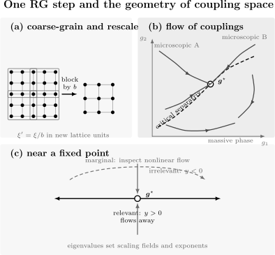
Three views of one RG idea. Blocking removes short-distance distinctions and restores the cutoff by rescaling. Repetition generates trajectories in coupling space, with a critical separatrix flowing toward a fixed point. Linearization near that point distinguishes relevant directions that grow, irrelevant directions that decay, and marginal directions requiring nonlinear analysis.

Continuous Flow and Beta Functions

For an infinitesimal scale change, the discrete map becomes

$$\frac{d g_i}{d\ell} = \beta_i(\boldsymbol g).$$

The functions $\beta_i$ are beta functions in the convention that $\ell$ increases toward the infrared. Some QFT texts instead differentiate with respect to an increasing energy scale $\mu$; that reverses signs because

$$\ell \sim \ln \frac{\Lambda}{\mu}.$$

A sign statement such as “the coupling grows” is incomplete unless the scale convention is stated.

The formal solution defines a trajectory

$$\boldsymbol g(\ell) = \Phi_\ell \bigl( \boldsymbol g(0) \bigr).$$

The components $g_i$ depend on how the effective action is parameterized. The physical content lies in long-distance observables, invariant scaling data, and the qualitative geometry of the flow.

Fixed Points

A fixed point satisfies

$$\boldsymbol\beta(\boldsymbol g^\star) = \boldsymbol 0.$$

At such a point, coarse-graining followed by rescaling reproduces the same theory. The fixed-point theory is scale invariant under the assumptions of the RG transformation.

Gaussian fixed point

A fixed point whose long-distance action is quadratic is called Gaussian. Wick’s theorem applies to its field correlations. Gaussian fixed points control many free theories and mean-field regimes, but an allowed interaction can destabilize them.

Interacting fixed point

At an interacting fixed point, dimensionless couplings approach nonzero values and anomalous scaling can appear. The Wilson–Fisher fixed point below four dimensions is the canonical equilibrium example.

The fixed-point coupling itself is not usually universal. It can change under a smooth reparameterization of coupling space. Critical exponents and properly normalized long-distance observables are the meaningful comparison.

Infrared and ultraviolet roles

An infrared fixed point attracts flows as $\ell\to\infty$. A ultraviolet fixed point governs short-distance behavior when the flow is followed in the opposite direction.

The same fixed point can be attractive in some directions and repulsive in others. “Stable fixed point” should therefore specify the subspace under discussion.

Lines and manifolds of fixed points

Sometimes

$$\boldsymbol\beta(\boldsymbol g^\star(s)) = 0$$

for a continuous parameter $s$. A fixed line can support continuously varying scaling dimensions. Luttinger liquids and compact-boson theories provide central one-dimensional examples.

Runaway flow

A truncated flow may run toward large coupling. This can indicate:

• formation of a gap or bound state;
• an ordering instability;
• flow toward a strong-coupling fixed point outside the chosen coordinates;
• a first-order transition;
• breakdown of the truncation;
• the need for new degrees of freedom.

Runaway flow is a diagnosis that the present weak-coupling description has failed, not a universal proof of which physical outcome occurs.

Linearization Near a Fixed Point

Write

$$g_i = g_i^\star + \delta g_i.$$

To first order,

$$\frac{d\,\delta g_i}{d\ell} = \sum_j B_{ij} \delta g_j + O(\delta g^2),$$

where

$$B_{ij} := \left. \frac{\partial\beta_i} {\partial g_j} \right|_{\boldsymbol g^\star}.$$

Choose eigen-directions $u_a$ of the stability matrix:

$$\frac{d u_a}{d\ell} = y_a u_a.$$

Then

$$u_a(\ell) = e^{y_a\ell} u_a(0).$$

With the infrared convention used here:

• $y_a>0$ is relevant;
• $y_a<0$ is irrelevant;
• $y_a=0$ is marginal at linear order.

These labels belong to a specified fixed point. The same microscopic perturbation can project onto different eigen-directions near different fixed points.

Relevant Directions

A relevant perturbation grows as the observation scale increases. To reach a critical fixed point with $n_{\mathrm{rel}}$ independent relevant directions, one generally must tune $n_{\mathrm{rel}}$ controls, unless symmetries or constraints set some of them to zero automatically.

For an Ising critical point at zero field, the temperature-like field and magnetic field are relevant. If exact $\mathbb Z_2$ symmetry enforces zero magnetic field, only the temperature-like control must be tuned experimentally.

The set of initial couplings that flow into the fixed point is its critical surface or stable manifold. Its codimension equals the number of relevant directions under standard regularity assumptions.

Irrelevant Directions

An irrelevant perturbation decays:

$$u_{\mathrm{irr}}(\ell) = e^{y_{\mathrm{irr}}\ell} u_{\mathrm{irr}}(0), \qquad y_{\mathrm{irr}}<0.$$

It does not disappear instantly. At finite size $L$, choose

$$\ell \sim \ln \frac{L}{a}.$$

Then

$$u_{\mathrm{irr}}(L) \sim u_{\mathrm{irr}}(a) \left( \frac{L}{a} \right)^{y_{\mathrm{irr}}}.$$

Defining

$$\omega := -y_{\mathrm{irr}} > 0,$$

gives the familiar correction

$$L^{-\omega}.$$

Different microscopic models in one universality class can have different correction amplitudes because they begin at different positions along irrelevant directions.

Marginal Directions

Linearization alone cannot classify $y=0$. Suppose

$$\frac{dg}{d\ell} = A g^2 + O(g^3).$$

The leading solution is

$$g(\ell) = \frac{g_0} {1-A g_0\ell}.$$

Depending on the signs of $A$ and $g_0$, the coupling can:

• drift logarithmically toward zero and be marginally irrelevant;
• grow logarithmically and be marginally relevant;
• remain exactly marginal when the beta function vanishes to all orders.

Marginality produces some of the slowest crossovers in many-body physics. It underlies logarithmic finite-size corrections, the Kondo scale, and fixed lines with continuously varying exponents.

Scaling Dimensions and RG Eigenvalues

If a scaling operator $\mathcal O_a$ has dimension $\Delta_a$ in a $D$-dimensional isotropic Euclidean theory,

$$\int d^D x\, g_a\mathcal O_a$$

is dimensionless when the coupling has eigenvalue

$$y_a = D-\Delta_a.$$

Thus:

• $\Delta_a<D$ corresponds to a relevant coupling;
• $\Delta_a>D$ corresponds to an irrelevant coupling;
• $\Delta_a=D$ is marginal by power counting.

For a quantum critical point with anisotropic scaling,

$$\mathbf x \longmapsto b\mathbf x, \qquad \tau \longmapsto b^z\tau,$$

the measure scales as if

$$D_{\mathrm{sc}} = d+z.$$

One may then write $y_a=d+z-\Delta_a$ when $\Delta_a$ is defined with that anisotropic scaling. This is not a claim that every quantum theory is literally an isotropic classical theory in $d+z$ dimensions.

Correlation-Length Exponent from Flow

Let $u_t$ be the leading temperature-like or tuning direction:

$$\frac{du_t}{d\ell} = y_tu_t, \qquad y_t>0.$$

Flow remains near the fixed point until $u_t(\ell)$ becomes order one. Define $\ell_\star$ by

$$\lvert u_t(0)\rvert e^{y_t\ell_\star} \sim 1.$$

The corresponding physical length is

$$\xi \sim a e^{\ell_\star}.$$

Eliminating $\ell_\star$ gives

$$\xi \sim a \lvert u_t(0)\rvert^{-1/y_t}.$$

Therefore

$$\nu = \frac{1}{y_t}.$$

This derivation identifies $\nu$ with a fixed-point stability eigenvalue. Critical Exponents and Scaling owns the general definition, extraction, and caveats for $\nu$.

Tree-Level Power Counting

Power counting classifies operators at a Gaussian fixed point before fluctuation corrections are included. Landau Theory owns the uniform invariant polynomial and its mean-field minima, Landau–Ginzburg Theory Preview owns the static gradient functional, Gaussian propagator, and Ginzburg criterion, and Statistical Field Theory Preview owns the regulated measure in which those fluctuations are integrated. The action here is used to classify those couplings by scale. Consider

$$\begin{aligned} S[\phi] &= \int d^d x\, \Bigl[ \frac12(\nabla\phi)^2 + \frac r2\phi^2 \\ &\qquad + \frac{u}{4!}\phi^4 + \sum_{n\ge3} g_{2n}\phi^{2n} \Bigr]. \end{aligned}$$

Keeping the gradient term dimensionless gives

$$\Delta_\phi^{(0)} = \frac{d-2}{2}.$$

The Gaussian eigenvalues are

$$y_r^{(0)} = 2,$$ $$y_u^{(0)} = 4-d,$$

and

$$y_{2n}^{(0)} = d - n(d-2).$$

Consequently, the quartic coupling is:

• relevant for $d<4$;
• marginal by power counting at $d=4$;
• irrelevant for $d>4$.

This identifies the upper critical dimension $d_c=4$ for the short-range scalar $\phi^4$ problem. Below four dimensions, the Gaussian classification signals that fluctuations drive the flow away from mean field. It does not calculate the interacting fixed point or its anomalous exponents.

Power counting is a first pass

Tree-level dimensions can be altered by:

• anomalous dimensions at an interacting fixed point;
• operator mixing;
• nonanalytic momentum or frequency kernels;
• constraints and gauge redundancies;
• Fermi-surface kinematics;
• long-range interactions;
• disorder averaging;
• boundary scaling.

An operator that is marginal by naive dimensions is a question, not an answer.

Flow Geometry and Universality

Microscopic models $A$ and $B$ can start at different points in coupling space yet flow toward the same fixed point after their relevant controls are tuned:

$$\boldsymbol g_A(\ell) \longrightarrow \boldsymbol g^\star, \qquad \boldsymbol g_B(\ell) \longrightarrow \boldsymbol g^\star.$$

Their common fixed-point data produce the shared exponents and scaling functions described by Universality. Their differing irrelevant coordinates produce nonuniversal amplitudes and correction terms.

A universality class is therefore associated with a fixed point plus the appropriate long-distance operator dictionary, symmetry data, and boundary or dynamic specification. The basin of attraction says which microscopic theories reach it.

Crossover and Separatrices

Suppose a perturbation $w$ is relevant at one fixed point, with eigenvalue $y_w>0$. Its crossover length is set by

$$\lvert w\rvert e^{y_w\ell_\times} \sim 1,$$

so

$$\xi_\times \sim a \lvert w\rvert^{-1/y_w}.$$

For scales below $\xi_\times$, data can resemble the unstable fixed point. At larger scales, the trajectory bends toward its ultimate infrared behavior.

A separatrix is a boundary in coupling space separating flows with different infrared outcomes. At a continuous transition, the critical surface is a separatrix between neighboring phases. Locating it numerically is equivalent to tuning away the relevant direction.

Near two competing fixed points, effective exponents can drift:

$$\kappa_{\mathrm{eff}}(L) := \frac{d\ln O(L)} {d\ln L}.$$

Plateaus over limited sizes may represent crossover rather than the final class.

Why RG Is Natural in Many-Body Physics

Critical fluctuations span many scales

Near a continuous transition,

$$a \ll r \ll \xi$$

contains no single privileged length. Perturbation theory organized around one scale accumulates contributions from many decades. RG treats those decades successively.

Effective degrees of freedom change with scale

Microscopic electrons can reorganize into quasiparticles, Cooper pairs, collective spin fields, gauge excitations, or hydrodynamic densities. RG does not require the same variables to remain efficient at every scale. A strong-coupling flow often signals that the useful degrees of freedom should change.

Logarithms need resummation

Terms such as

$$g^n \ln^n \left( \frac{\Lambda}{E} \right)$$

can invalidate a fixed-order expansion even when $g$ is small. RG absorbs the large logarithms into a running coupling evaluated at the scale $E$.

Lattice details can become irrelevant

A lattice fixes the ultraviolet regulator, point-group symmetry, allowed operators, and bare couplings. Near a continuum critical point, irrelevant lattice anisotropies can decay, leaving an emergent rotational or internal symmetry. The decay rate itself controls corrections.

Finite size and temperature stop the flow

A finite system of size $L$ stops spatial coarse-graining near

$$\ell_L \sim \ln \frac{L}{a}.$$

At a quantum critical point, temperature supplies an imaginary-time extent $\beta\hbar$. If characteristic energy scales transform as

$$E(\ell) \sim \Lambda_E e^{-z\ell},$$

then thermal effects stop the zero-temperature flow near

$$\ell_T \sim \frac{1}{z} \ln \frac{\Lambda_E}{k_{\mathrm B}T}.$$

Finite-size and finite-temperature scaling are therefore RG flows terminated before the infinite-scale fixed point is reached.

Many-Body Examples

Ising criticality

Different short-range Ising lattices have different bare couplings and critical temperatures. After tuning the temperature-like direction, their flows approach the same Ising fixed point. Lattice-specific terms survive as metric factors and irrelevant corrections.

Kondo exchange

For a metallic antiferromagnetic Kondo coupling, the dimensionless exchange is marginally relevant. A schematic weak-coupling equation is

$$\frac{dg}{d\ell} = A g^2, \qquad A>0.$$

The coupling reaches order one at

$$\ell_K \sim \frac{1}{A g_0},$$

which defines the exponentially small energy

$$k_{\mathrm B}T_K \sim D_0 \exp \left( -\frac{1}{A g_0} \right).$$

The weak-coupling pole marks the end of that coordinate chart, not an infinite physical interaction. Kondo Model Preview owns conventions, screening, thermodynamics, and the strong-coupling interpretation.

Luttinger liquids

A broad family of one-dimensional gapless systems flows to a fixed line described by a compact boson. The Luttinger parameter labels points on that line and controls scaling dimensions. Some perturbations are relevant for one parameter range and irrelevant for another. Luttinger Liquid Preview fixes a field convention and works out the resulting impurity, Umklapp, pairing, and correlation exponents.

This makes relevance state-dependent in coupling space: an impurity, umklapp term, or pairing operator cannot be classified without specifying the fixed-line parameter.

Fermi surfaces

For a Fermi liquid, low energy means proximity to the Fermi surface, not small absolute momentum. One integrates out a thin energy shell around the surface:

$$\Lambda_E/b < \lvert\varepsilon_{\mathbf k}-\mu\rvert < \Lambda_E.$$

Kinematic restrictions make forward scattering and the Cooper channel special. Ordinary isotropic power counting around $\mathbf k=0$ would miss this structure.

Bose–Hubbard transitions

At a generic Mott-lobe side, the leading temporal derivative and dilute-particle kinematics produce a different scaling structure from the particle–hole-symmetric lobe tip. RG makes precise why changing the boundary point can change $z$, the relevant operators, and the universality class even within one microscopic Hamiltonian.

Integrating Out Versus Projecting Out

Wilsonian shell integration, a Schrieffer–Wolff transformation, and a variational truncation can all reduce a problem, but they are not identical.

Functional integration

One sums over eliminated fluctuations and obtains a scale-dependent action for retained fields. The result generally contains infinitely many induced operators.

Unitary block diagonalization

A controlled unitary transformation can decouple low- and high-energy subspaces order by order in a ratio such as $V/\Delta$. Operators must be transformed along with the Hamiltonian.

Variational truncation

Numerical methods may retain states judged important by energy, entanglement, or another criterion. Their errors depend on the truncation and are not automatically captured by field-theory relevance.

All three require a declared scale window and an error estimate. Calling each procedure “RG” without specifying the map hides their distinct guarantees.

Scheme and Coordinate Dependence

Let new coupling coordinates be

$$g'_a = f_a(\boldsymbol g).$$

The beta function transforms as a vector field:

$$\beta'_a(\boldsymbol g') = \sum_i \frac{\partial f_a} {\partial g_i} \beta_i(\boldsymbol g).$$

Therefore:

• fixed-point coordinates can move;
• individual beta-function coefficients can depend on convention;
• trajectories can look different in different coordinates;
• regular reparameterizations preserve the number of relevant directions and the stability eigenvalues at a fixed point.

A running coupling is not directly observable merely because it has a plotted value. It becomes physical through a matching condition and predictions for observables.

Dangerous Irrelevance

An irrelevant coupling usually supplies a vanishing correction. It is dangerously irrelevant when setting it to zero changes the phase structure, normalization, or scaling of an observable.

Above the upper critical dimension, the quartic coupling in a scalar theory is irrelevant at the Gaussian fixed point, yet it stabilizes the ordered free energy and affects finite-size and order-parameter scaling. One cannot simply delete it before asking those questions.

The adjective “dangerous” is observable-dependent. The coupling can be irrelevant for the fixed-point free energy while remaining essential to a derived amplitude or ordered-phase limit.

Boundaries, Disorder, and Dynamics

Boundary flows

A boundary supports its own operators and couplings. Bulk criticality can coexist with ordinary, special, or extraordinary surface behavior. An impurity problem is often naturally a boundary RG problem.

Disorder

Quenched disorder introduces distributions of couplings and, in quantum path integrals, correlations extended along imaginary time. Average and typical observables can scale differently. Strong-disorder flows may broaden rather than approach a narrow conventional distribution.

Dynamic flows

Equilibrium couplings do not determine the full dynamics. Conservation laws, reversible mode coupling, damping kernels, and noise strengths enlarge coupling space. Static and dynamic fixed points must be distinguished.

What Full RG Adds

This preview stops before several technical subjects become the main object:

• regulator construction and cutoff independence;
• loop expansion and diagrammatic beta functions;
• renormalization conditions and counterterms;
• field and composite-operator renormalization;
• operator mixing matrices;
• functional and exact flow equations;
• gauge symmetry, Ward identities, and anomalies;
• rigorous continuum limits;
• nonperturbative QFT fixed points.

Those subjects require a complete field-theoretic framework. Use Continue on QFT.org when the RG machinery itself, rather than its many-body interpretation, becomes central.

A Reliable RG Workflow

1. Declare the scale convention

State whether increasing the flow parameter means:

• increasing length;
• decreasing energy;
• increasing renormalization scale;
• increasing system size;
• moving along an iterative numerical chain.

This fixes the sign convention for every beta function and stability eigenvalue.

2. Identify the low-energy manifold

The eliminated modes must be chosen around the actual low-energy structure:

• $\mathbf q=0$ for a conventional ferromagnetic order parameter;
• a nonzero ordering wavevector for density-wave order;
• a Fermi surface for a metal;
• isolated nodes for a semimetal;
• a boundary or impurity channel for a local problem;
• frequency as well as momentum for dissipative dynamics.

A spherical shell around the wrong point is not an innocuous scheme choice.

3. State degrees of freedom and symmetries

List the retained fields, constraints, global and gauge symmetries, conservation laws, and boundary conditions. Then enumerate the operators those data allow.

The RG cannot protect a term that the stated symmetry permits but the truncation silently omits.

4. Make couplings dimensionless

If a coupling $\lambda$ has engineering dimension $y_\lambda$, define a dimensionless variable using the running scale $\mu$:

$$g(\mu) := \lambda(\mu) \mu^{-y_\lambda},$$

up to normalization conventions. Fixed points are naturally statements about dimensionless couplings.

A dimensionful parameter can change simply because units change. That kinematic scaling should not be mistaken for an interaction correction.

5. Separate exact steps from approximations

The identity defining $S_{\mathrm{eff}}$ can be exact, while its evaluation is approximate. Record whether the approximation is:

• a cumulant expansion;
• a loop truncation;
• a derivative expansion;
• an operator truncation;
• a large-$N$ expansion;
• a numerical state truncation;
• a projection in a small ratio.

Then identify the parameter or convergence study that controls it.

6. Find fixed points and invariant subspaces

Solve

$$\boldsymbol\beta(\boldsymbol g^\star) = 0$$

within the declared truncation. Check whether symmetries define invariant planes or lines. A fixed point found outside the regime where the beta functions were derived is not automatically trustworthy.

7. Linearize and count tuning directions

Compute the stability matrix and its eigenvalues. Use eigenvectors, not the original bare couplings, when operator mixing is present.

The number of positive $y_a$ in the infrared convention predicts the codimension of the critical surface. Compare that number with the controls actually tuned in the model or experiment.

8. Match to observables

Connect scaling fields to measurable controls and operators:

• Which combination of temperature and pressure is $u_t$?
• Which microscopic observable overlaps with the order parameter?
• Which source excites the leading relevant operator?
• Which irrelevant field supplies the dominant correction?

Without this matching, a flow diagram is not yet a physical prediction.

9. Stop at physical infrared cutoffs

The flow can terminate at:

• correlation length $\xi$;
• system size $L$;
• thermal length;
• inverse frequency;
• mean free path;
• gap scale;
• disorder or inhomogeneity scale.

Compare each cutoff before claiming that the asymptotic fixed point is experimentally accessible.

10. Test truncation and scheme robustness

Vary the cutoff profile, operator basis, loop order, derivative order, or numerical truncation when possible. Universal quantities should converge even though fixed-point coordinates and intermediate trajectories move.

Common Mistakes

Calling any fitted parameter renormalized

RG running has a declared scale and matching prescription. A phenomenological parameter adjusted once is not automatically a running coupling.

Confusing RG time with physical time

$d\boldsymbol g/d\ell$ describes changing resolution, not unitary or dissipative evolution of a quantum state.

Keeping only the microscopic operators

Coarse-graining generates all symmetry-allowed terms. A closed truncation requires an argument.

Classifying a marginal operator by power counting alone

When $y=0$, nonlinear beta-function terms decide whether the coupling is marginally relevant, marginally irrelevant, or exactly marginal.

Treating a strong-coupling pole as a physical divergence

A perturbative pole marks loss of the weak-coupling description. The infrared physics can remain finite after a change of variables.

Reading fixed-point coordinates as universal

Smooth coupling redefinitions move $\boldsymbol g^\star$. Stability eigenvalues and observable scaling data are the robust content.

Assuming irrelevant means removable

Irrelevant couplings generate finite-scale corrections, and dangerously irrelevant variables can remain essential for selected observables or phases.

Using small momentum for every many-body problem

Metals are organized around a Fermi surface; antiferromagnets around an ordering wavevector; impurities around a local channel. The low-energy shell must follow the spectrum.

Inferring a first-order transition from runaway flow alone

Runaway flow may instead indicate a gap, bound state, new fixed point, or failed truncation.

Forgetting finite cutoffs

A system can remain in crossover because $L$, $1/T$, or the observation time stops the flow before the asymptotic regime.

Equating DMRG with Wilsonian field RG

Density-matrix renormalization group is a powerful variational state-truncation method. Its name reflects a scale-building strategy, but its mathematical guarantee is not identical to integrating a momentum shell in a path integral.

Exercises

Exercise 1: Correlation length and one relevant direction

Near a fixed point, a tuning field obeys

$$\frac{du}{d\ell} = y u, \qquad y>0.$$

Assume the microscopic value is $u_0$ and define $\ell_\star$ by $\lvert u(\ell_\star)\rvert=1$.

1. Find $\ell_\star$.
2. If $\xi=a e^{\ell_\star}$, derive $\nu$.
3. Explain what changes if the laboratory control $t$ satisfies $u_0=c_1t+c_2t^2+\cdots$ with $c_1\ne0$.

Solution

The linear flow gives

$$u(\ell) = u_0e^{y\ell}.$$

The stopping condition is

$$\lvert u_0\rvert e^{y\ell_\star} = 1,$$

so

$$\ell_\star = -\frac{1}{y} \ln\lvert u_0\rvert.$$

Therefore

$$\xi = a \lvert u_0\rvert^{-1/y}.$$

Comparing with $\xi\sim\lvert u_0\rvert^{-\nu}$ gives

$$\nu = \frac1y.$$

If $u_0=c_1t+O(t^2)$ with $c_1\ne0$, then

$$\xi \sim a \lvert c_1t\rvert^{-1/y} \left[ 1+O(t) \right].$$

The analytic coefficient changes the nonuniversal amplitude, while the exponent remains $1/y$. If $c_1=0$ because of symmetry or a special path, the leading power of $t$ must be reconsidered.

Exercise 2: Gaussian power counting

For the scalar action in $d$ dimensions, use

$$\Delta_\phi^{(0)} = \frac{d-2}{2}$$

to find the Gaussian RG eigenvalues of couplings multiplying $\phi^2$, $\phi^4$, $\phi^6$, and $\phi^8$. Classify them in $d=3$.

Solution

A coupling to $\phi^{2n}$ has

$$y_{2n}^{(0)} = d - 2n\Delta_\phi^{(0)} = d - n(d-2).$$

Thus

$$\begin{aligned} y_2^{(0)} &= 2, \\ y_4^{(0)} &= 4-d, \\ y_6^{(0)} &= 6-2d, \\ y_8^{(0)} &= 8-3d. \end{aligned}$$

At $d=3$,

$$\begin{aligned} y_2^{(0)}&=2, & y_4^{(0)}&=1, \\ y_6^{(0)}&=0, & y_8^{(0)}&=-1. \end{aligned}$$

Therefore $\phi^2$ and $\phi^4$ are relevant at the Gaussian fixed point, $\phi^6$ is marginal by tree-level power counting, and $\phi^8$ is irrelevant. The $\phi^6$ term still requires nonlinear analysis, and these Gaussian labels need not equal the labels at an interacting fixed point.

Exercise 3: Two fixed points in one beta function

Consider

$$\frac{dg}{d\ell} = \epsilon g - A g^2, \qquad \epsilon>0, \quad A>0.$$

Find the fixed points and determine their stability along the $g$ direction.

Solution

The fixed-point condition is

$$g \left( \epsilon-Ag \right) = 0.$$

Hence

$$g_0^\star = 0, \qquad g_1^\star = \frac{\epsilon}{A}.$$

The stability eigenvalue in one dimension is

$$y(g^\star) = \left. \frac{d\beta}{dg} \right|_{g^\star} = \epsilon-2Ag^\star.$$

At the Gaussian point,

$$y(g_0^\star) = \epsilon > 0,$$

so positive $g$ is relevant and the Gaussian point is infrared-repulsive along this direction.

At the interacting point,

$$y(g_1^\star) = -\epsilon < 0,$$

so the point is infrared-attractive along $g$. A full critical theory can still possess another relevant direction, such as a mass, that must be tuned.

Exercise 4: Codimension and correction exponent

A fixed point has stability eigenvalues

$$\begin{aligned} y_1&=1.60, & y_2&=-0.82, \\ y_3&=-2.1. \end{aligned}$$

Assume no symmetry removes any direction.

1. How many independent controls must be tuned?
2. What is the leading correlation-length exponent if $y_1$ is temperature-like?
3. What is the leading correction exponent?

Solution

Only $y_1$ is positive, so the critical surface has codimension one. One independent control must be tuned.

The correlation-length exponent is

$$\nu = \frac{1}{y_1} = \frac{1}{1.60} = 0.625.$$

Among irrelevant directions, the one closest to zero decays most slowly. Therefore

$$\omega = -y_2 = 0.82.$$

The $y_3$ direction produces a faster correction proportional to $L^{-2.1}$ unless analytic or symmetry effects introduce an even slower term.

Exercise 5: Marginally relevant scale

Let

$$\frac{dg}{d\ell} = A g^2, \qquad A>0.$$

Analyze $g_0>0$ and $g_0<0$. For $g_0>0$, find the energy scale $E_\star$ at which the weak-coupling solution reaches order one if

$$E(\ell) = D_0e^{-\ell}.$$

Solution

The solution is

$$g(\ell) = \frac{g_0} {1-Ag_0\ell}.$$

For $g_0<0$, the denominator grows and

$$g(\ell) \longrightarrow 0^-$$

logarithmically. The coupling is marginally irrelevant.

For $g_0>0$, the denominator decreases. The one-loop solution becomes strong near

$$\ell_\star \sim \frac{1}{Ag_0}.$$

The corresponding energy is

$$E_\star \sim D_0 \exp \left( -\frac{1}{Ag_0} \right).$$

This essential dependence is dimensional transmutation: a dimensionless bare coupling creates an exponentially small energy. The divergence of the approximate $g(\ell)$ is not itself a divergent observable.

Exercise 6: Reparameterizing a beta function

Let

$$g' = f(g) = g+c g^2,$$

where $f'(g^\star)\ne0$. Show that a fixed point maps to a fixed point and that the one-dimensional stability eigenvalue is unchanged.

Solution

The transformed beta function is

$$\beta'(g') = \frac{df}{dg} \beta(g).$$

If $\beta(g^\star)=0$, then

$$\beta' \left( f(g^\star) \right) = 0,$$

so

$$g'^\star = f(g^\star)$$

is a fixed point.

Differentiate with respect to $g'$:

$$\frac{d\beta'}{dg'} = \frac{1}{f'(g)} \frac{d}{dg} \left[ f'(g)\beta(g) \right].$$

At the fixed point, the term containing $\beta(g^\star)$ vanishes, leaving

$$\left. \frac{d\beta'}{dg'} \right|_{g'^\star} = \left. \frac{d\beta}{dg} \right|_{g^\star}.$$

Thus the fixed-point coordinate changes but the linear stability eigenvalue does not, provided the coordinate transformation is regular.

Exercise 7: Thermal cutoff of a quantum flow

A quantum critical theory has $z=2$, ultraviolet energy $\Lambda_E$, and a weak coupling that would reach strong coupling at RG time $\ell_\star=8$. At temperature $T$, take

$$\ell_T = \frac12 \ln \frac{\Lambda_E}{k_{\mathrm B}T}.$$

1. What condition on $T$ allows the flow to reach strong coupling before thermal cutoff?
2. Evaluate the threshold ratio $k_{\mathrm B}T/\Lambda_E$.

Solution

The flow reaches strong coupling first when

$$\ell_T > \ell_\star.$$

Therefore

$$\frac12 \ln \frac{\Lambda_E}{k_{\mathrm B}T} > 8.$$

Multiplying by two and exponentiating gives

$$\frac{\Lambda_E}{k_{\mathrm B}T} > e^{16},$$

or

$$\frac{k_{\mathrm B}T}{\Lambda_E} < e^{-16} \simeq 1.13\times10^{-7}.$$

The tiny threshold shows how an apparently valid zero-temperature strong-coupling prediction can be preempted by a finite experimental temperature.

Exercise 8: Crossover from an unstable fixed point

A symmetry-breaking perturbation $w$ has eigenvalue $y_w=0.25$ at an otherwise attractive fixed point. The microscopic value is $\lvert w_0\rvert=10^{-4}$.

1. Estimate $\xi_\times/a$.
2. Explain why simulations with $L/a\le10^8$ can misidentify the universality class.
3. Name two diagnostics of crossover.

Solution

The crossover length is

$$\frac{\xi_\times}{a} \sim \lvert w_0\rvert^{-1/y_w}.$$

Since $1/y_w=4$,

$$\frac{\xi_\times}{a} \sim \left( 10^{-4} \right)^{-4} = 10^{16}.$$

All sizes up to $10^8a$ remain eight orders of magnitude below the crossover scale. They can display excellent apparent scaling governed by the unstable fixed point even though the ultimate infrared class is different.

Useful diagnostics include:

• drift of effective exponents with increasing minimum size;
• growth of observables in the symmetry-breaking channel;
• failure of one correction exponent to fit all sizes;
• crossings that drift systematically rather than converging;
• direct scaling of the perturbing operator.

A good collapse below $\xi_\times$ demonstrates a preasymptotic regime, not the final class.

Key Takeaways

• RG compares effective descriptions at different resolutions; it is not physical time evolution.
• A Wilsonian step integrates out a scale shell, rescales coordinates and fields, and changes every symmetry-allowed coupling.
• Repeated steps generate beta-function flow in an infinite-dimensional coupling space.
• Fixed points are scale-invariant descriptions; their coordinates are scheme-dependent, while stability exponents and observable scaling data are robust.
• Positive, negative, and zero stability eigenvalues are relevant, irrelevant, and marginal in the stated infrared convention.
• The number of relevant directions determines how many controls must be tuned to reach a critical surface.
• The leading tuning eigenvalue gives $\nu=1/y_t$, while the least irrelevant direction gives the correction exponent $\omega=-y_{\mathrm{irr}}$.
• Marginal couplings require nonlinear analysis and can produce logarithms, fixed lines, or exponentially small scales.
• Runaway weak-coupling flow signals failure of that description, not a unique physical endpoint.
• Many-body shells must follow the actual low-energy manifold, such as a Fermi surface, ordering wavevector, node, or impurity channel.
• Finite size, temperature, frequency, and gaps stop the flow and can leave observables in crossover.
• Full loop-level and relativistic RG machinery belongs in the dedicated QFT treatment.

Further Reading

• Scaling Theory of Localization applies autonomous beta-function flow, fixed-point stability, relevant and irrelevant fields, and scheme independence to disordered conductance.
• Universality — class membership and universal versus nonuniversal data.
• Critical Exponents and Scaling – exponent definitions, finite-size scaling, and correction-aware inference.
• Quantum Phase Transitions – zero-temperature scaling and quantum-critical fans.
• Why Many-Body QM Leads to QFT – microscopic, auxiliary, and collective fields.
• Interacting Many-Body Systems Overview – coupling regimes and method selection.
• Lattice Models Overview – lattice operators, locality, and continuum limits.
• Kondo Model Preview – marginal flow and dimensional transmutation.
• XXZ Spin Chain – Luttinger fixed lines and Berezinskii–Kosterlitz–Thouless behavior.
• Euclidean and Imaginary-Time Path Integrals – the functional-integral bridge.
• Critical Phenomena and RG Bridge – continuum limits, scaling operators, relevant QFT deformations, and a one-loop Wilson–Fisher preview.
• Continue on QFT.org – publication-aware route to the full field-theoretic continuation.

References

1. L. P. Kadanoff, “Scaling Laws for Ising Models Near $T_c$,” Physics Physique Fizika 2, 263–272 (1966), doi:10.1103/PhysicsPhysiqueFizika.2.263.
2. K. G. Wilson, “Renormalization Group and Critical Phenomena. I. Renormalization Group and the Kadanoff Scaling Picture,” Physical Review B 4, 3174–3183 (1971), doi:10.1103/PhysRevB.4.3174.
3. K. G. Wilson, “Renormalization Group and Critical Phenomena. II. Phase-Space Cell Analysis of Critical Behavior,” Physical Review B 4, 3184–3205 (1971), doi:10.1103/PhysRevB.4.3184.
4. F. J. Wegner, “Corrections to Scaling Laws,” Physical Review B 5, 4529–4536 (1972), doi:10.1103/PhysRevB.5.4529.
5. K. G. Wilson and M. E. Fisher, “Critical Exponents in 3.99 Dimensions,” Physical Review Letters 28, 240–243 (1972), doi:10.1103/PhysRevLett.28.240.
6. K. G. Wilson and J. Kogut, “The Renormalization Group and the $\epsilon$ Expansion,” Physics Reports 12, 75–199 (1974), doi:10.1016/0370-1573(74)90023-4.
7. K. G. Wilson, “The Renormalization Group: Critical Phenomena and the Kondo Problem,” Reviews of Modern Physics 47, 773–840 (1975), doi:10.1103/RevModPhys.47.773.
8. M. E. Fisher, “The Renormalization Group in the Theory of Critical Behavior,” Reviews of Modern Physics 46, 597–616 (1974), doi:10.1103/RevModPhys.46.597.
9. J. Polchinski, “Renormalization and Effective Lagrangians,” Nuclear Physics B 231, 269–295 (1984), doi:10.1016/0550-3213(84)90287-6.
10. R. Shankar, “Renormalization-Group Approach to Interacting Fermions,” Reviews of Modern Physics 66, 129–192 (1994), doi:10.1103/RevModPhys.66.129.
11. P. W. Anderson, “A Poor Man’s Derivation of Scaling Laws for the Kondo Problem,” Journal of Physics C: Solid State Physics 3, 2436–2441 (1970), doi:10.1088/0022-3719/3/12/008.
12. J. M. Kosterlitz, “The Critical Properties of the Two-Dimensional XY Model,” Journal of Physics C: Solid State Physics 7, 1046–1060 (1974), doi:10.1088/0022-3719/7/6/005.
13. J. A. Hertz, “Quantum Critical Phenomena,” Physical Review B 14, 1165–1184 (1976), doi:10.1103/PhysRevB.14.1165.
14. S. R. White, “Density Matrix Formulation for Quantum Renormalization Groups,” Physical Review Letters 69, 2863–2866 (1992), doi:10.1103/PhysRevLett.69.2863.
15. G. Vidal, “Entanglement Renormalization,” Physical Review Letters 99, 220405 (2007), doi:10.1103/PhysRevLett.99.220405.
16. C. Wetterich, “Exact Evolution Equation for the Effective Potential,” Physics Letters B 301, 90–94 (1993), doi:10.1016/0370-2693(93)90726-X.
17. M. E. Fisher, “Renormalization Group Theory: Its Basis and Formulation in Statistical Physics,” Reviews of Modern Physics 70, 653–681 (1998), doi:10.1103/RevModPhys.70.653.
18. J. Cardy, Scaling and Renormalization in Statistical Physics, Cambridge University Press (1996), doi:10.1017/CBO9781316036440.