Spontaneous Symmetry Breaking

Spontaneous symmetry breaking occurs when a family of many-body Hamiltonians has an exact symmetry, yet its stable thermodynamic states preserve only a proper subgroup of that symmetry.

The three ingredients are logically distinct:

$$\begin{gathered} \text{symmetric dynamics}, \\ \text{a many-body or thermodynamic limit}, \\ \text{stable states related by the symmetry}. \end{gathered}$$

A nonsymmetric vector in one finite Hilbert space is not enough. Nor is a degenerate spectrum, a large susceptibility, or a convenient mean-field ansatz by itself. The defining phenomenon is the emergence of distinct, locally observable phases that remain after the perturbation used to select them is removed in the appropriate order of limits.

In compact form, if $G$ acts by $U_\Lambda(g)$ and

$$U_\Lambda(g) H_\Lambda U_\Lambda(g)^{-1} = H_\Lambda,$$

then a limiting state $\omega_\alpha$ breaks $G$ when there are a local observable $A$ and an element $g\in G$ such that

$$\omega_\alpha(A) \ne \omega_\alpha \left( U(g)^{-1}AU(g) \right).$$

The subgroup that leaves the state invariant is the unbroken subgroup

$$H_\alpha = \left\{ g\in G: \omega_\alpha\circ\alpha_g = \omega_\alpha \right\}.$$

The symmetry-related family of ordered states is organized, at least locally, by the orbit $G/H_\alpha$.

Canonical Scope

This page is the canonical many-body treatment of spontaneous symmetry breaking. It owns:

• symmetry of the Hamiltonian versus symmetry of a state;
• why finite systems often hide thermodynamic order;
• source-selected limits and Bogoliubov quasiaverages;
• branch selection by weak fields, boundaries, preparation, and measurement;
• finite-size cat states and their local thermodynamic limits;
• quasi-degenerate multiplets for broken discrete symmetries;
• Anderson towers of states for broken continuous symmetries;
• the distinction between symmetry-breaking, accidental, and topological degeneracy;
• practical finite-size, numerical, and experimental diagnostics.

Neighboring pages retain separate ownership:

• Order Parameters defines microscopic ordering operators, normalizations, sources, and finite-size estimators.
• Thermodynamic Limit develops limiting sequences, boundary conditions, and noncommuting bulk limits.
• Connected Correlation Functions owns cluster decomposition, pure-phase subtraction, and symmetric mixtures.
• Long-Range Order owns correlation limits, squared-order scaling, and finite-size correlation criteria.
• Off-Diagonal Long-Range Order owns density-matrix criteria for bosonic and fermion-pair condensates.
• Goldstone Modes in Many-Body Systems owns gapless collective modes and nonrelativistic counting.
• Landau Theory owns uniform symmetry-allowed potentials and their candidate minima; multiple minima alone do not establish thermodynamic symmetry breaking.
• Explicit Symmetry Breaking owns symmetry loss in the equations themselves.
• Degeneracy Lifting owns finite-dimensional projected perturbation theory.
• Model pages retain exact spectra, phase diagrams, and model-specific order parameters.

The shorter Spontaneous Symmetry Breaking Preview introduces the language from the symmetry side. The present page supplies the many-body mechanism.

Hamiltonian Symmetry and State Symmetry

Let $\Lambda$ denote a finite region, lattice, or collection of degrees of freedom. A symmetry group $G$ is represented by unitary or antiunitary transformations $U_\Lambda(g)$ satisfying

$$U_\Lambda(g) H_\Lambda U_\Lambda(g)^{-1} = H_\Lambda.$$

For a density operator $\rho_\Lambda$, symmetry of the state means

$$U_\Lambda(g) \rho_\Lambda U_\Lambda(g)^{-1} = \rho_\Lambda.$$

These are different statements:

Object	Symmetry condition	Meaning
Hamiltonian	$UHU^{-1}=H$	the dynamics or equilibrium weights respect $G$
pure state	$U\lvert\psi\rangle=e^{i\phi}\lvert\psi\rangle$	the ray is invariant
density operator	$U\rho U^{-1}=\rho$	all expectation values respect $G$
ordered phase	invariant only under $H\subsetneq G$	some local expectations distinguish symmetry-related states

If $\rho_\alpha$ is a broken-symmetry state, then

$$\rho_{g\alpha} = U(g)\rho_\alpha U(g)^{-1}$$

has the same energy density but generally different local expectation values. The symmetry maps one ordered state to another; it has not disappeared from the theory.

An order parameter witnesses the mismatch

Suppose an intensive order parameter $\phi_a$ transforms in a representation $D(g)$:

$$\phi_a \longmapsto \sum_b D_{ab}(g)\phi_b.$$

If a selected state has $\boldsymbol\phi\ne0$, only the subgroup satisfying

$$D(g)\boldsymbol\phi = \boldsymbol\phi$$

leaves that state invariant. The order parameter is a witness of the symmetry mismatch, but its construction and normalization belong to Order Parameters.

What a Unique Finite Ground State Can Do

Suppose $H_\Lambda$ has a nondegenerate ground state $|\Omega_\Lambda\rangle$. Since

$$\left[ H_\Lambda,U_\Lambda(g) \right] = 0,$$

the vector $U_\Lambda(g)|\Omega_\Lambda\rangle$ is also a ground state. Nondegeneracy therefore implies

$$U_\Lambda(g) |\Omega_\Lambda\rangle = e^{i\phi_\Lambda(g)} |\Omega_\Lambda\rangle.$$

The ground-state ray is symmetric. If an operator $\widehat M_\Lambda$ is odd under a discrete symmetry,

$$U_\Lambda \widehat M_\Lambda U_\Lambda^{-1} = -\widehat M_\Lambda,$$

then

$$\langle\Omega_\Lambda| \widehat M_\Lambda |\Omega_\Lambda\rangle = 0.$$

This theorem is elementary but central: a finite, unique symmetry eigenstate cannot literally choose one symmetry-related branch.

It does not imply that finite systems contain no evidence of order. They can show:

• $\langle\widehat M_\Lambda^2\rangle\propto V_\Lambda^2$;
• a structure-factor peak proportional to volume;
• an anomalously large susceptibility;
• quasi-degenerate levels in different symmetry sectors;
• a sharply bimodal order-parameter distribution;
• extreme sensitivity to a field that decreases with size.

The finite state can contain the correlations needed to build ordered thermodynamic states while keeping its one-point function exactly symmetric.

Exact Finite Degeneracy Is Not the Definition

If a finite ground space is degenerate, one can often choose a nonsymmetric linear combination immediately. That observation alone does not establish spontaneous symmetry breaking.

Finite degeneracy may be:

• enforced by an irreducible symmetry representation;
• protected by Kramers theorem;
• caused by a disconnected geometry or fine tuning;
• associated with edge modes;
• topological and locally indistinguishable;
• accidental and removed by a generic symmetric perturbation;
• the finite-size precursor of symmetry breaking.

A symmetry-breaking interpretation requires a family of growing systems and stable limiting states. The relevant branches must be distinguishable by local or coarse-grained observables and related by the broken symmetry.

A useful local criterion

Let $|\Omega_{\alpha,\Lambda}\rangle$ and $|\Omega_{\beta,\Lambda}\rangle$ be candidate branches. Symmetry-breaking branches should admit a fixed-support observable $A_X$ for which

$$\lim_{\Lambda\nearrow\infty} \left[ \langle A_X\rangle_{\alpha,\Lambda} - \langle A_X\rangle_{\beta,\Lambda} \right] \ne 0.$$

By contrast, topologically degenerate ground states on a closed manifold are locally indistinguishable in the bulk:

$$\langle A_X\rangle_{\alpha,\Lambda} - \langle A_X\rangle_{\beta,\Lambda} \longrightarrow 0$$

for every fixed local $A_X$, up to finite-size corrections. Degeneracy is therefore evidence whose physical origin must be diagnosed, not a synonym for broken symmetry.

A useful taxonomy

Spectrum at finite size	Local distinguishability	Typical interpretation
exact multiplet fixed by symmetry	may or may not hold	representation theory first
isolated accidental crossing	generally model dependent	not robust enough for a phase
quasi-degenerate symmetry multiplet collapsing with size	yes in suitable combinations	symmetry-breaking precursor
topology-dependent near-degeneracy	no for bulk local probes	topological order
edge-state degeneracy	distinguishable near boundaries	boundary phenomenon

The Superselection Sectors Preview gives the operator-algebraic meaning of a superselection rule. It is best not to call every finite-size symmetry sector a superselection sector.

The Thermodynamic Construction

Choose a sequence of finite regions

$$\Lambda_1 \subset \Lambda_2 \subset \cdots, \qquad V_\Lambda\longrightarrow\infty,$$

with specified interactions and boundary conditions. A thermodynamic state is defined by the limiting expectation values of every fixed local observable:

$$\omega(A_X) = \lim_{\Lambda\nearrow\infty} \operatorname{Tr} \left( \rho_\Lambda A_X \right), \qquad X\subset\Lambda.$$

The limit is local. One does not need a norm limit of vectors living in different Hilbert spaces.

Different choices of:

• boundary condition;
• weak source;
• subsequence of volumes;
• preparation history;
• thermal ensemble;

can lead to different limiting states at the same Hamiltonian parameters. In an ordered region these states may have the same bulk free-energy density while differing in an order parameter.

The symmetric limiting state

Taking the unbiased finite-volume ground state or Gibbs state to infinite volume can produce a symmetric state

$$\omega_{\mathrm{sym}} = \int d\mu(\alpha)\, \omega_\alpha,$$

where $\omega_\alpha$ are symmetry-related extremal phases and $d\mu$ is an invariant measure on their orbit.

For a $\mathbb Z_2$ order parameter, the simplest example is

$$\omega_{\mathrm{sym}} = \frac12 \left( \omega_+ + \omega_- \right).$$

This state is legitimate, but it is not a selected pure phase. Its long-distance connected correlations can retain the classical uncertainty about the global branch.

Extremal phases

An equilibrium state is extremal within a convex set of equilibrium states if it cannot be written as a nontrivial convex mixture of other states in that set. Ordered pure phases are normally represented by extremal states.

For two clustering branches with

$$\omega_\pm(O) = \pm m_0,$$

one has

$$\lim_{|\mathbf r|\to\infty} \omega_\pm \left( O(\mathbf r)O(\mathbf0) \right) = m_0^2,$$

while the connected part tends to zero. In the symmetric mixture, the one-point function vanishes but the full and connected correlators both retain the plateau $m_0^2$.

The canonical subtraction and cluster-property analysis is in Connected Correlation Functions.

Source-Selected States

Let $\widehat M_\Lambda$ be an extensive order operator and add a conjugate source:

$$H_\Lambda(h) = H_\Lambda - h\widehat M_\Lambda.$$

For $h\ne0$, the source explicitly breaks the symmetry. The spontaneous order parameter is defined by removing that source after the thermodynamic limit:

$$m_+ = \lim_{h\to0^+} \lim_{\Lambda\nearrow\infty} \frac{ \langle\widehat M_\Lambda\rangle_{\Lambda,h} }{ V_\Lambda }.$$

For a $\mathbb Z_2$ symmetry,

$$m_- = \lim_{h\to0^-} \lim_{\Lambda\nearrow\infty} \frac{ \langle\widehat M_\Lambda\rangle_{\Lambda,h} }{ V_\Lambda } = -m_+.$$

At fixed finite volume, analyticity and symmetry usually give

$$\lim_{h\to0} \frac{ \langle\widehat M_\Lambda\rangle_{\Lambda,h} }{ V_\Lambda } = 0.$$

Consequently,

$$\begin{aligned} \lim_{h\to0^+} \lim_{\Lambda\nearrow\infty} \frac{\langle\widehat M_\Lambda\rangle}{V_\Lambda} &= m_0, \\ \lim_{\Lambda\nearrow\infty} \lim_{h\to0^+} \frac{\langle\widehat M_\Lambda\rangle}{V_\Lambda} &= 0 \end{aligned}$$

in the standard ordered situation. The noncommuting limits are the operational signature of spontaneous selection.

Bogoliubov quasiaverages

The source-selected prescription is often called a quasiaverage:

$$\prec A\succ = \lim_{h\to0^+} \lim_{\Lambda\nearrow\infty} \langle A\rangle_{\Lambda,h}.$$

The small source is not claimed to be absent during the finite-volume calculation. Its role is to choose one limiting phase. What makes the result spontaneous is that the selected order remains finite as the source is removed after the bulk limit.

Free-energy viewpoint

Let

$$f(h) = -\lim_{\Lambda\nearrow\infty} \frac{1}{\beta V_\Lambda} \log Z_\Lambda(h).$$

Where the derivative exists,

$$m(h) = -\frac{\partial f}{\partial h}.$$

For a discrete broken symmetry, $f(h)$ can develop a cusp at $h=0$:

$$\begin{gathered} \lim_{h\to0^+}m(h)=m_0, \\ \lim_{h\to0^-}m(h)=-m_0. \end{gathered}$$

Each finite-volume free energy remains analytic in $h$ under ordinary conditions. The nonanalyticity emerges only after the thermodynamic limit.

How an Infinitesimal Source Wins

The finite-size competition is transparent in a two-state approximation. Let $|\Omega_+\rangle$ and $|\Omega_-\rangle$ denote two localized branches with order parameters $\pm m_0$. In their span, write

$$H_{\mathrm{eff}} = E_0\mathbf1 - \frac{\Delta_\Lambda}{2}\tau_x - hV_\Lambda m_0\tau_z.$$

Here:

• $\Delta_\Lambda$ is the finite-size tunneling splitting;
• $\tau_x$ mixes the branches;
• $hV_\Lambda m_0$ is the extensive source bias.

The level separation is

$$E_+-E_- = 2 \sqrt{ \left( \frac{\Delta_\Lambda}{2} \right)^2 + \left( hV_\Lambda m_0 \right)^2 }.$$

The ground-state order parameter is

$$\frac{\langle\widehat M_\Lambda\rangle}{V_\Lambda} = m_0 \frac{ hV_\Lambda m_0 }{ \sqrt{ \left( \Delta_\Lambda/2 \right)^2 + \left( hV_\Lambda m_0 \right)^2 } }.$$

Selection occurs once

$$|h|V_\Lambda m_0 \gg \Delta_\Lambda.$$

Thus the field needed to orient the system scales as

$$h_{\mathrm{sel}}(\Lambda) \sim \frac{\Delta_\Lambda}{V_\Lambda m_0}.$$

If $\Delta_\Lambda$ collapses rapidly, the selecting field can vanish even faster. “Infinitesimal” is therefore a statement about a size-dependent competition, not an assertion that a mathematically zero perturbation changes a finite nondegenerate eigenstate.

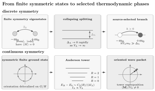
Finite systems can preserve the exact symmetry while carrying the precursors of order. Discrete order commonly produces a small tunneling splitting $\Delta_\Lambda$ between symmetry eigenstates. Continuous order commonly produces a rotor-like tower with spacings of order $1/V_\Lambda$. A source whose extensive bias exceeds these collapsing scales selects one member of the thermodynamic family.

Selection Mechanisms

A conjugate bulk field is the cleanest theoretical selector, but it is not the only one.

Bulk source

A term

$$-h\widehat M_\Lambda$$

directly favors one order-parameter orientation. It gives the sharpest definition of a quasiaverage and the associated susceptibility.

Boundary conditions

Fixed or weakly biased boundary conditions can select a bulk phase. For short-range systems, the boundary contribution is subextensive, but in an ordered region it can determine which extensive interior state is realized.

The correct question is not whether the boundary energy is extensive. It is whether the bulk has several asymptotically degenerate phases for the boundary to choose among.

Preparation and initial conditions

Unitary dynamics under a symmetric Hamiltonian preserves the symmetry of a perfectly symmetric density operator. A nonsymmetric preparation can nevertheless remain oriented for a time that grows strongly with system size because transitions between macroscopically distinct branches are suppressed.

This is a dynamical statement and should not be confused with the equilibrium definition. Metastability, prethermal order, and driven symmetry breaking require their own time-limit prescriptions.

Measurement and environment

A local measurement can condition a symmetric cat-like state onto one branch, and weak environmental couplings can decohere interference between macroscopically distinct orientations. These processes explain why finite macroscopic apparatuses display definite outcomes.

They do not replace the thermodynamic criterion. An environment can also explicitly bias, heat, or destroy the ordered phase. One must separate:

1. existence of several stable bulk branches;
2. suppression of coherence between them;
3. stochastic or biased selection of one branch.

Selection versus creation

A perturbation selects pre-existing spontaneous order if the induced order remains nonzero after the source is removed in the thermodynamic prescription. It merely creates polarization if

$$\lim_{h\to0} \lim_{\Lambda\nearrow\infty} \frac{\langle\widehat M_\Lambda\rangle}{V_\Lambda} = 0.$$

A large but finite susceptibility can make the latter response impressive without producing a broken phase.

Cat States and Local Physics

Consider two macroscopically distinct branch states $|\Omega_+\rangle$ and $|\Omega_-\rangle$. Symmetry eigenstates can be approximated by

$$|\mathrm{cat}_\pm\rangle = \frac{ |\Omega_+\rangle \pm |\Omega_-\rangle }{ \sqrt{ 2 \left( 1\pm\operatorname{Re} \langle\Omega_+|\Omega_-\rangle \right) } }.$$

When the branch overlap vanishes with size,

$$\langle\Omega_+|\Omega_-\rangle \longrightarrow 0.$$

For a fixed local observable $A_X$, interference matrix elements also normally vanish:

$$\langle\Omega_+| A_X |\Omega_-\rangle \longrightarrow 0.$$

The cat state then has the local expectation

$$\langle A_X\rangle_{\mathrm{cat}} \longrightarrow \frac12 \left( \omega_+(A_X) + \omega_-(A_X) \right).$$

Locally, the symmetric cat approaches the same mixture as an unbiased classical ensemble, even though the finite global state is pure.

Reduced density operators

For any fixed region $X$, tracing out its complement gives

$$\rho_X^{\mathrm{cat}} \longrightarrow \frac12 \left( \rho_X^+ + \rho_X^- \right).$$

The phase coherence resides in observables whose support grows with the system. Ordinary local probes cannot recover it in the thermodynamic limit.

This fact resolves an apparent contradiction:

• the exact finite ground state may be a symmetric pure vector;
• every fixed local experiment can converge to a symmetric mixture;
• selected boundary conditions or sources converge to an extremal ordered phase.

There is no single state-independent meaning of “the” thermodynamic ground-state vector.

Macroscopic fluctuations

If

$$\widehat M_\Lambda |\Omega_\pm\rangle \simeq \pm m_0V_\Lambda |\Omega_\pm\rangle,$$

then a symmetric cat has

$$\langle\widehat M_\Lambda\rangle_{\mathrm{cat}} \simeq 0,$$

but

$$\langle\widehat M_\Lambda^2\rangle_{\mathrm{cat}} \simeq m_0^2V_\Lambda^2.$$

The variance is macroscopic. It records uncertainty between branches, not ordinary $O(V_\Lambda)$ fluctuations within one clustering phase.

Broken Discrete Symmetries

For a discrete symmetry, the orbit $G/H$ contains a discrete set of ordered branches. A $\mathbb Z_2$ ferromagnet has two:

$$m=+m_0, \qquad m=-m_0.$$

Finite-size spectrum

At finite size, tunneling between branches commonly produces symmetric and antisymmetric combinations. Their splitting

$$\Delta_\Lambda = E_{\mathrm{odd}} - E_{\mathrm{even}}$$

collapses rapidly in the ordered regime.

In a one-dimensional transverse-field Ising chain deep in the ordered phase, the splitting is exponentially small in chain length:

$$\Delta_L \sim e^{-L/\xi_{\mathrm{tun}}}$$

up to model- and boundary-dependent prefactors. Other geometries can produce different exponential variables and prefactors. Exponential collapse is typical for a gapped discrete ordered phase, not a universal exact formula.

Domain walls

Spatially varying configurations can interpolate between discrete branches. The interface is a domain wall. In a conventional short-range ordered phase, a large static interface has an energy cost set by its area:

$$E_{\mathrm{wall}} \sim \sigma L^{d-1},$$

where $\sigma$ is a domain-wall tension.

Domain walls explain:

• finite-temperature disordering in many discrete systems;
• nucleation and hysteresis;
• slow switching in finite samples;
• sensitivity to boundaries and defects.

They do not imply a Goldstone mode. The branch set is discrete, so there is no arbitrarily small uniform rotation along an order-parameter manifold.

No universal degeneracy count

The number of branches is often the number of disconnected points in $G/H$, but spatial symmetry breaking can also produce:

• several ordering wavevectors;
• translations of a commensurate pattern;
• orientations related by a point group;
• domains combining several broken operations.

Count physically distinct states after quotienting by the subgroup that leaves the complete ordered pattern invariant.

Broken Continuous Symmetries

If $G$ is continuous and a state preserves $H\subsetneq G$, symmetry-related orientations form a continuous manifold

$$\mathcal M = G/H.$$

Examples include:

$$\begin{array}{ccl} SO(3)\to SO(2) &:& \mathcal M\simeq S^2, \\ U(1)\to\{1\} &:& \mathcal M\simeq S^1. \end{array}$$

The tangent directions to $\mathcal M$ are broken symmetry directions. They organize low-energy dynamics, but the number of Nambu–Goldstone modes need not equal the number of broken generators in a nonrelativistic system.

The collective rotor

On a finite sample, the global orientation cannot remain perfectly sharp while the exact state stays symmetric. Its slow uniform motion is often described by a quantum rotor:

$$H_{\mathrm{rot}} = \frac{ \widehat{\mathbf L}_{\mathcal M}^{\,2} }{ 2I_\Lambda },$$

where $I_\Lambda$ is a collective moment of inertia. For a conventional antiferromagnet,

$$I_\Lambda \propto \chi_\perp V_\Lambda.$$

Rotor levels therefore scale as

$$E_R-E_0 \sim \frac{ C_2(R) }{ 2I_\Lambda } \propto \frac{1}{V_\Lambda},$$

where $C_2(R)$ is the quadratic Casimir of the symmetry representation $R$.

For $SO(3)$,

$$E_S-E_0 \simeq \frac{ S(S+1) }{ 2\chi_\perp V_\Lambda }.$$

The sequence of low-lying symmetry multiplets is the Anderson tower of states, also called the thin spectrum or quasi-degenerate joint states.

What the tower means

The tower is a finite-size spectral fingerprint of an emergent continuous family of orientations:

• every finite eigenstate can carry a definite symmetry quantum number;
• the tower spacings collapse as the volume grows;
• wave packets formed from many tower states can localize on $\mathcal M$;
• the energy-density cost of localization vanishes in the thermodynamic limit.

If

$$|\Omega_{\mathbf n}\rangle = \sum_R c_R(\mathbf n)|R\rangle,$$

then choosing coefficients spread across the tower localizes the order parameter near orientation $\mathbf n$. Such a state is not an exact finite-volume energy eigenstate, but its excess energy density can vanish:

$$\frac{ \langle H_\Lambda\rangle_{\mathbf n} - E_0 }{ V_\Lambda } \longrightarrow 0.$$

Tower levels are not Goldstone waves

The tower describes the spatially uniform collective orientation. Goldstone modes carry nonzero momentum and describe long-wavelength distortions.

For a system with linear Goldstone dispersion,

$$\Delta_{\mathrm{tower}} \sim L^{-d}, \qquad \Delta_{\mathrm{Goldstone}} \sim L^{-1}.$$

They are parametrically distinct for $d>1$. Conflating them obscures both finite-size spectroscopy and low-energy field theory.

The tower is also not universal in the same form. Ferromagnets, systems with type-B modes, conserved order parameters, long-range interactions, and nonstandard geometries can have exceptional finite-size structures. The rigorous Koma–Tasaki construction applies under stated locality, long-range-order, and commutator assumptions; it is not a license to fit every low-energy multiplet to one rotor formula.

Discrete and Continuous Breaking Compared

Feature	Discrete symmetry	Continuous symmetry
ordered-state set	separated branches	manifold $G/H$
common finite-size signature	quasi-degenerate symmetry combinations	tower of representations
common collapse scale	often exponential	commonly $1/V_\Lambda$ for rotor levels
defects	domain walls and junctions	vortices, textures, and other defects
Goldstone modes	not implied	expected under appropriate assumptions
weak source	chooses a branch	orients the order parameter

These columns describe common short-range equilibrium cases. Long-range interactions, constraints, subsystem symmetries, fractonic structures, and nonequilibrium phases require additional qualifications.

Perturbations and Stability

Let a perturbation be

$$\delta H_\Lambda = \lambda V_\Lambda^{(\mathrm{pert})}.$$

Three questions must be kept separate.

Does it preserve the symmetry?

If

$$\left[ V_\Lambda^{(\mathrm{pert})}, U_\Lambda(g) \right] = 0$$

for all $g$, the perturbation cannot directly prefer one symmetry-related branch. It can still move a phase boundary, change stiffnesses, or destroy the ordered phase.

If the perturbation transforms like the order parameter, it explicitly biases an orientation.

How does its matrix element scale?

A uniform conjugate source contributes an energy difference of order

$$\delta E_{\mathrm{bias}} \sim hV_\Lambda m_0.$$

A boundary pinning field may scale like $L^{d-1}$. A local impurity contributes only $O(1)$ energy, although it can nucleate a domain in a susceptible system. The relevant comparison is always with the finite-size splitting and interface costs.

Does the phase survive removal?

The state is spontaneously ordered only if the selected local observables remain nonzero after the perturbation is removed according to the thermodynamic prescription.

Projected matrix elements within a finite degenerate subspace are treated in Degeneracy Lifting. Here the new ingredient is the scaling of that subspace and its splittings with system size.

Random fields are not innocuous selectors

A spatially random source does more than choose a uniform branch. It competes with domain-wall energy and can fragment or destroy order. Whether weak randomness preserves a phase depends on dimension, symmetry, interaction range, and disorder correlations.

“Any tiny perturbation selects the phase” is therefore too broad. The perturbation’s symmetry, spatial profile, and scaling matter.

Pure Phases, Mixtures, and Superselection Language

In an infinite system, symmetry-related extremal phases can become disjoint representations of the local observable algebra. No quasilocal operation converts one macroscopic phase into another with finite cost and nonvanishing amplitude.

This motivates a superselection-like description of broken phases, but terminology should be used carefully:

• a finite even and odd parity sector is an ordinary symmetry decomposition;
• an infinite-volume decomposition into disjoint phases is a stronger statement;
• algebraic superselection depends on the chosen observable algebra;
• gauge-charge superselection and symmetry-breaking phase selection are not identical constructions.

For most calculations, it is enough to state the operational consequence:

$$\begin{gathered} \text{fixed-support observables} \\ \text{cannot detect coherent} \\ \text{phase interference} \end{gathered}$$

as the volume tends to infinity.

The canonical algebraic vocabulary is deferred to Superselection Sectors Preview.

Finite Temperature

At finite volume, the Gibbs state

$$\rho_{\Lambda,\beta} = \frac{ e^{-\beta H_\Lambda} }{ Z_{\Lambda,\beta} }$$

inherits every unitary symmetry of $H_\Lambda$:

$$U_\Lambda(g) \rho_{\Lambda,\beta} U_\Lambda(g)^{-1} = \rho_{\Lambda,\beta}.$$

Finite-temperature symmetry breaking therefore also requires an infinite-volume limit. Below a transition, several extremal Gibbs or KMS states can coexist. Their symmetric convex combination is again a valid Gibbs state.

The source-selected thermal order parameter is

$$m_\beta = \lim_{h\to0^+} \lim_{\Lambda\nearrow\infty} \frac{ \operatorname{Tr} \left( e^{-\beta H_\Lambda(h)} \widehat M_\Lambda \right) }{ V_\Lambda Z_\Lambda(h) }.$$

The planned Finite-Temperature Phase Transitions page will own thermal singularities, coexistence, and scaling.

Dimensional and Locality Constraints

Spontaneous symmetry breaking is not guaranteed merely because a symmetric Landau potential has several minima.

Continuous symmetries at nonzero temperature

For broad classes of one- and two-dimensional systems with sufficiently short-range interactions, thermal fluctuations forbid conventional spontaneous breaking of continuous internal symmetries. The Mermin–Wagner theorem establishes this for isotropic short-range Heisenberg models, while Hohenberg’s result excludes the corresponding condensate order in one and two dimensions at $T>0$ under its assumptions.

The conclusion depends on:

• continuous rather than discrete symmetry;
• spatial dimension;
• finite nonzero temperature;
• interaction range and regularity;
• the type of order being tested.

Two-dimensional $U(1)$ systems can still exhibit a Berezinskii–Kosterlitz–Thouless phase with algebraic order and finite stiffness, without a nonzero local order parameter in the infinite system.

Zero temperature is different

A $d$-dimensional quantum ground-state problem is often related to a $(d+z)$-dimensional classical field theory, but this mapping is guidance, not a universal no-go theorem.

Examples:

• a one-dimensional quantum Ising chain can break its discrete $\mathbb Z_2$ symmetry at $T=0$;
• a generic short-range antiferromagnetic chain does not develop conventional continuous Néel order;
• a Heisenberg ferromagnet is an important exceptional continuous-symmetry case;
• long-range interactions can alter lower critical dimensions.

Always state temperature, dimension, interaction range, and symmetry class before invoking a no-go result.

One-dimensional thermal discrete order

For a one-dimensional short-range Ising system at $T>0$, domain walls have finite energy and nonzero density, so conventional long-range order is destroyed. This is a model mechanism, not the Mermin–Wagner theorem, which concerns continuous symmetries.

Global Symmetry Versus Gauge Redundancy

Spontaneous symmetry breaking applies directly to physical global symmetries. A local gauge transformation is a redundancy of description, not an operation relating physically distinct states in the same way.

Elitzur’s theorem shows, under its lattice-gauge assumptions, that a local gauge symmetry cannot acquire a gauge-noninvariant order parameter without gauge fixing. Consequently:

• a gauge-dependent field expectation is not by itself an observable phase diagnostic;
• physical statements should be phrased with gauge-invariant operators, Wilson lines, stiffnesses, flux response, or other appropriate observables;
• the Higgs mechanism is not simply ordinary breaking of a physical local symmetry.

Particle-number symmetry

For a neutral Bose gas, global particle-number $U(1)$ is a physical symmetry. A fixed-number finite state satisfies

$$\langle\widehat\psi(\mathbf r)\rangle = 0,$$

yet it can possess Bose–Einstein condensation through a macroscopic eigenvalue of the one-body density matrix. A source-selected phase-coherent representation and a number-conserving representation can encode the same local thermodynamic physics.

The bosonic benchmark belongs to Bose–Einstein Condensation; Off-Diagonal Long-Range Order develops the general one-body and fermion-pair density-matrix criteria.

Charged condensates

In a superconductor, electromagnetic gauge invariance, global charge conservation, phase stiffness, and the observable electromagnetic response must be disentangled. A nonzero gauge-fixed pair amplitude is computationally useful, but it is not by itself a gauge-invariant measurement.

Model Example: Transverse-Field Ising Chain

Consider

$$H = -J \sum_{j} \sigma_j^z\sigma_{j+1}^z - gJ \sum_j \sigma_j^x,$$

with spin-flip parity

$$\mathcal P = \prod_j\sigma_j^x.$$

Because

$$\mathcal P \sigma_j^z \mathcal P^{-1} = -\sigma_j^z,$$

finite parity eigenstates have zero longitudinal magnetization.

In the ordered regime $0\le g<1$, the lowest even and odd states become quasi-degenerate as $L$ grows. Their combinations

$$|\Omega_\uparrow\rangle \simeq \frac{ |\mathrm{even}\rangle + |\mathrm{odd}\rangle }{ \sqrt2 },$$

and

$$|\Omega_\downarrow\rangle \simeq \frac{ |\mathrm{even}\rangle - |\mathrm{odd}\rangle }{ \sqrt2 }$$

carry opposite magnetization.

The selected infinite-chain result is

$$m_z = \lim_{\lambda\to0^+} \lim_{L\to\infty} \left\langle \frac1L\sum_j\sigma_j^z \right\rangle_{ H-\lambda\sum_j\sigma_j^z }.$$

Exact magnetization, Jordan–Wigner solution, and boundary-sector details remain in the Transverse-Field Ising Model.

Model Example: Heisenberg Antiferromagnet

For a bipartite antiferromagnet, define the staggered order operator

$$\widehat{\mathbf M}_s = \sum_{j\in A} \widehat{\mathbf S}_j - \sum_{j\in B} \widehat{\mathbf S}_j.$$

A finite, even, rotationally invariant sample can have a unique singlet ground state:

$$\widehat{\mathbf S}_{\mathrm{tot}}^2 |\Omega\rangle = 0.$$

Then

$$\langle\widehat{\mathbf M}_s\rangle = \mathbf0,$$

even though

$$\langle \widehat{\mathbf M}_s^{\,2} \rangle \propto V_\Lambda^2$$

in an ordered sequence.

The low-energy spectrum contains total-spin multiplets with the rotor form

$$E_S-E_0 \simeq \frac{ S(S+1) }{ 2\chi_\perp V_\Lambda }.$$

Superposing these tower states produces a Néel-oriented wave packet. This is the canonical example behind Anderson’s tower and the rigorous Koma–Tasaki relation between long-range order, low-lying states, and broken-symmetry thermodynamic states.

The Heisenberg Model owns lattice conventions, ferro- versus antiferromagnetic regimes, and model-specific diagnostics.

The ferromagnetic exception

An isotropic Heisenberg ferromagnet can possess an exactly degenerate maximal-spin ground multiplet even at finite size. Fully polarized states are exact eigenstates and already have nonzero magnetization.

This does not invalidate the thermodynamic framework. It shows that a unique symmetric finite ground state and a $1/V$ tower are common mechanisms, not necessary axioms. The phase claim still concerns robustness, locality, and the behavior of a growing family of systems.

Model Example: Neutral Bose Condensate

For a finite system with fixed particle number,

$$\left[ H,\widehat N \right] = 0$$

and

$$\langle\widehat\psi(\mathbf r)\rangle = 0.$$

A symmetry-breaking calculation introduces a source

$$\begin{aligned} H_\eta &= H - \int d^dr\, \widehat{\mathcal J}_\eta(\mathbf r), \\ \widehat{\mathcal J}_\eta(\mathbf r) &= \eta^*(\mathbf r)\widehat\psi(\mathbf r) + \eta(\mathbf r)\widehat\psi^\dagger(\mathbf r). \end{aligned}$$

Taking the thermodynamic limit before $\eta\to0$ can define a phase-oriented state with

$$\langle\widehat\psi(\mathbf r)\rangle = \sqrt{n_0}\,e^{i\theta}.$$

The phase $\theta$ labels a $U(1)$ orbit. Yet condensation itself can be defined without a nonzero field expectation, using the one-body density matrix. The two languages must not be conflated with two different physical condensates.

Spatial Symmetry Breaking

The same logic applies to translations and rotations. A crystal Hamiltonian can be translation invariant while an equilibrium state has a periodic density:

$$\langle\widehat n(\mathbf r)\rangle = n_0 + \sum_{\mathbf G\ne0} n_{\mathbf G} e^{i\mathbf G\cdot\mathbf r}.$$

Translating the density pattern produces another state with the same free-energy density. Finite samples, walls, strain, impurities, and measurement apparatuses strongly pin an origin and orientation.

Spatial symmetries add subtleties:

• the symmetry group is noncompact or includes spacetime operations;
• acoustic phonons are tied to broken translations;
• defects and elasticity carry geometric information;
• boundaries explicitly remove translation invariance.

The general source and state logic survives, but crystalline order deserves its own correlation and elasticity treatment.

Explicit and Spontaneous Breaking Compared

Question	Explicit breaking	Spontaneous breaking
Is $H$ invariant under $G$?	no	yes before the selector is added
Why is one orientation favored?	Hamiltonian parameters	selected thermodynamic state
Does a finite source remain?	generally yes	removed after bulk limit
Are symmetry-related branches exactly equivalent?	generally no	yes at zero source
Can a would-be Goldstone mode be gapped?	yes, as a pseudo-Goldstone mode	not from exact continuous breaking alone

Real materials commonly contain both. Crystal fields, strain, dipolar interactions, substrates, and laboratory fields can weakly break an idealized symmetry. The useful procedure is:

1. identify the exact symmetry of the physical Hamiltonian;
2. identify any approximate larger symmetry;
3. determine whether the unbiased ideal limit supports ordered branches;
4. estimate how explicit terms split or pin those branches.

Calling every small anisotropy “spontaneous” discards physically measurable energy scales.

Numerical Diagnostics

Finite computations never take the thermodynamic limit literally. A convincing diagnosis combines several scaling tests.

One-point functions with controlled pinning

Apply a field $h_L$ or boundary pinning that decreases with size. Seek a window

$$\frac{\Delta_L}{V_Lm_0} \ll h_L \ll \Delta_{\mathrm{bulk}},$$

where $\Delta_{\mathrm{bulk}}$ is a microscopic or collective bulk scale. The first inequality selects a branch; the second keeps the probe weak.

Symmetry-even order estimators

At zero source, evaluate

$$m_L^2 = \frac{ \langle\widehat M_L^2\rangle }{ V_L^2 }.$$

A nonzero extrapolation is evidence for order even when $\langle\widehat M_L\rangle=0$.

Structure-factor scaling

For ordering wavevector $\mathbf Q$,

$$S(\mathbf Q) \propto V_L$$

in a convention where $S$ contains one factor of $1/V_L$. Always audit the normalization before inferring a volume law. Structure Factors owns the convention dictionary.

Spectral quantum numbers

Track:

• symmetry sectors of the lowest levels;
• splitting within the candidate quasi-degenerate set;
• scaling of that splitting with $L$ and $V_L$;
• separation from ordinary bulk excitations;
• representation pattern expected from $G/H$.

A collection of low levels is not automatically a tower. Its quantum numbers and scaling should match the proposed order.

Order-parameter distributions

The probability distribution

$$P_L(m) = \left\langle \delta \left( m-\frac{\widehat M_L}{V_L} \right) \right\rangle$$

can evolve from one peak to multiple symmetry-related peaks. At finite size, peak shape depends on ensemble, boundary conditions, sampling ergodicity, and measurement basis.

Susceptibility

The conjugate response

$$\chi_L = \left. \frac{\partial}{\partial h} \frac{ \langle\widehat M_L\rangle_h }{ V_L } \right|_{h=0}$$

often grows rapidly in an ordered regime because the source couples nearly degenerate states. Large $\chi_L$ is supporting evidence, not a standalone proof. Susceptibilities develops static, dynamic, isothermal, and isolated response limits.

Entanglement and tensor-network caveats

A finite-bond-dimension tensor network can prefer a minimally entangled broken branch even when the exact finite ground state is symmetric. Conversely, explicitly enforcing the symmetry can return a cat-like state or require a larger bond dimension.

Report:

• whether the ansatz enforces $G$;
• whether boundaries pin an orientation;
• whether truncation acts as an implicit selector;
• how observables change with bond dimension and size.

Experimental Interpretation

Experiments observe finite samples over finite times. Almost every apparatus contains weak symmetry-breaking fields and boundaries.

Evidence for spontaneous order is strongest when several observations agree:

• reproducible symmetry-related domains;
• an order parameter that remains finite as calibrated bias is reduced;
• a diverging or strongly enhanced conjugate susceptibility near a transition;
• collective modes appropriate to the broken continuous symmetry;
• domain walls or other defects with the expected topology;
• scaling with sample size, temperature, and control parameters;
• scattering peaks or interference signatures tied to the ordering channel.

Hysteresis is not enough

Hysteresis can arise from first-order coexistence, disorder pinning, kinetic arrest, or nonequilibrium metastability. It does not by itself identify the broken symmetry or prove an equilibrium thermodynamic phase.

A measured orientation is not a violation of symmetry

Observing one magnetization direction in one run does not mean the microscopic equations favored it. Across repeated unbiased preparations, different symmetry-related orientations may occur. The ensemble of runs can be symmetric while individual macroscopic outcomes are not.

A Reliable Workflow

When claiming spontaneous symmetry breaking, state each item explicitly.

1. Hamiltonian family: specify $H_\Lambda$, geometry, interactions, and boundary conditions.
2. Exact symmetry: give $G$ and its action on operators.
3. Candidate stabilizer: identify the subgroup $H$ preserved by the ordered state.
4. Order channel: define $\widehat M_\Lambda$, normalization, and ordering wavevector.
5. Limit: state $T$, $V_\Lambda\to\infty$, and the order of source, momentum, frequency, and time limits.
6. Phase selector: specify bulk field, boundary condition, preparation, or conditional measurement.
7. Finite-size evidence: examine squared order, correlations, distributions, susceptibility, and low-energy representations.
8. Stability: test symmetry-preserving perturbations and removal of the selector.
9. Alternatives: rule out accidental, edge, topological, and explicitly broken explanations.
10. Consequences: only then discuss domains, Goldstone modes, defects, or criticality.

This checklist prevents a variational ansatz or finite-size crossing from being promoted too quickly into a phase statement.

Common Mistakes

• Calling any nonsymmetric finite-system vector spontaneous symmetry breaking.
• Saying the Hamiltonian symmetry “disappears” in the broken phase.
• Treating exact finite degeneracy as sufficient without testing locality and robustness.
• Expecting a finite unique ground state to have a nonzero symmetry-odd one-point function.
• Reversing the source and thermodynamic limits without noticing.
• Treating the source that selects a branch as the origin of the ordered phase.
• Assuming all finite-size splittings are exponential.
• Calling every low-energy multiplet an Anderson tower.
• Confusing tower levels with finite-momentum Goldstone modes.
• Applying Goldstone reasoning to a discrete symmetry.
• Invoking Mermin–Wagner without stating dimension, temperature, interaction range, and symmetry.
• Treating local gauge redundancy like a physical global symmetry.
• Calling finite symmetry sectors superselection sectors without specifying the observable algebra and limit.
• Inferring order solely from a mean-field minimum or a large susceptibility.
• Confusing a symmetric phase mixture with a selected clustering phase.
• Using a tensor-network broken state without reporting whether the algorithm implicitly selected it.

Exercises

Exercise 1: Unique finite ground state

Let $U$ be a unitary symmetry with $[H,U]=0$, and suppose $|\Omega\rangle$ is a nondegenerate ground state. Prove that the ground-state ray is invariant. Then show that any operator $O$ satisfying $UOU^{-1}=-O$ has zero ground-state expectation value.

Solution

Since

$$H \left( U|\Omega\rangle \right) = UH|\Omega\rangle = E_0 \left( U|\Omega\rangle \right),$$

$U|\Omega\rangle$ is another ground state. Nondegeneracy implies

$$U|\Omega\rangle = e^{i\phi}|\Omega\rangle.$$

Therefore

$$\begin{aligned} \langle O\rangle &= \langle\Omega| U^{-1} \left( UOU^{-1} \right) U |\Omega\rangle \\ &= -\langle\Omega| U^{-1}OU |\Omega\rangle \\ &= -\langle O\rangle. \end{aligned}$$

Hence $\langle O\rangle=0$.

Exercise 2: Two-state selection scale

For

$$H_{\mathrm{eff}} = -\frac{\Delta}{2}\tau_x - hVm_0\tau_z,$$

derive the ground-state expectation of $\tau_z$. Find the crossover field and evaluate the two orders of limits when $\Delta_V\to0$ faster than $V$ grows.

Solution

The effective field in Pauli space is

$$\mathbf b = \left( \frac{\Delta}{2}, 0, hVm_0 \right).$$

The ground state aligns with $\mathbf b$, so

$$\langle\tau_z\rangle = \frac{ hVm_0 }{ \sqrt{ \left( \Delta/2 \right)^2 + \left( hVm_0 \right)^2 } }.$$

The crossover occurs at

$$|h|Vm_0 \sim \frac{\Delta}{2},$$

or

$$h_{\mathrm{sel}} \sim \frac{\Delta}{2Vm_0}.$$

At every finite $V$,

$$\lim_{h\to0^+} \langle\tau_z\rangle = 0.$$

If $\Delta_V/V\to0$, then any fixed $h>0$ satisfies the selection inequality for sufficiently large $V$, giving

$$\lim_{h\to0^+} \lim_{V\to\infty} \langle\tau_z\rangle = 1.$$

Reversing the limits gives zero.

Exercise 3: Hidden order in a cat state

Let

$$|\mathrm{cat}_+\rangle = \frac{ |\uparrow\uparrow\cdots\uparrow\rangle + |\downarrow\downarrow\cdots\downarrow\rangle }{ \sqrt2 },$$

and define

$$M = \frac1N \sum_{j=1}^N\sigma_j^z.$$

Compute $\langle M\rangle$, $\langle M^2\rangle$, and $\langle\sigma_i^z\sigma_j^z\rangle$ for $i\ne j$. What does a fixed proper subsystem see?

Solution

The two branches have $M=\pm1$, and the cross terms vanish. Hence

$$\langle M\rangle = \frac12(1-1) = 0,$$

while

$$\langle M^2\rangle = \frac12(1+1) = 1.$$

For $i\ne j$, both branches give aligned spins:

$$\langle\sigma_i^z\sigma_j^z\rangle = 1.$$

Tracing out at least one spin removes the off-diagonal branch coherence. Write the all-up and all-down product states on a fixed proper subsystem $X$ as $|\Uparrow_X\rangle$ and $|\Downarrow_X\rangle$. The subsystem sees

$$\begin{aligned} \rho_X &= \frac12 \lvert\Uparrow_X\rangle \langle\Uparrow_X\rvert \\ &\quad + \frac12 \lvert\Downarrow_X\rangle \langle\Downarrow_X\rvert. \end{aligned}$$

Locally this is a mixture, despite the purity of the global cat state.

Exercise 4: Tower versus Goldstone scaling

An antiferromagnet in $d$ spatial dimensions has $V=L^d$, a rotor moment of inertia $I=\chi_\perp V$, and a linear Goldstone velocity $c$. Compare the lowest rotor and nonzero-momentum Goldstone gaps.

Solution

The first rotor level has

$$\Delta_{\mathrm{rot}} \sim \frac1I \sim \frac1{\chi_\perp L^d}.$$

The smallest nonzero momentum is of order $2\pi/L$, so

$$\Delta_{\mathrm{G}} \sim c\frac{2\pi}{L}.$$

Thus

$$\frac{ \Delta_{\mathrm{rot}} }{ \Delta_{\mathrm{G}} } \sim L^{1-d}.$$

For $d>1$, the rotor tower collapses parametrically faster than the finite-momentum Goldstone gap. The tower describes global reorientation; the Goldstone excitation describes a spatial distortion.

Exercise 5: Degeneracy without symmetry breaking

Why does a fourfold ground-state degeneracy on a torus not by itself prove spontaneous breaking of a $\mathbb Z_4$ symmetry? Give a local test that distinguishes conventional symmetry-breaking degeneracy from topological degeneracy.

Solution

The number of states does not identify their origin. Four states can arise from symmetry breaking, topology, edges, fine tuning, or a representation-theoretic multiplet.

For conventional symmetry breaking, there should be a fixed local or coarse-grained operator $O_X$ whose expectation differs between suitable ground-state combinations:

$$\lim_{L\to\infty} \left[ \langle O_X\rangle_\alpha - \langle O_X\rangle_\beta \right] \ne0.$$

Topological ground states on a closed manifold are locally indistinguishable:

$$\langle O_X\rangle_\alpha - \langle O_X\rangle_\beta \longrightarrow0$$

for every fixed bulk-local $O_X$. One should also test how the degeneracy depends on topology and how states transform under actual symmetries.

Exercise 6: Stabilizer and order-parameter manifold

A collinear isotropic antiferromagnet chooses a unit Néel vector $\mathbf n$. Treating the continuous spin symmetry as $SO(3)$, find the subgroup that preserves $\mathbf n$ and the order-parameter manifold. How many broken generators are there? Does that number alone determine the number of Goldstone modes?

Solution

Rotations about $\mathbf n$ leave it fixed, so the stabilizer is

$$H \simeq SO(2).$$

The orbit is

$$\mathcal M = \frac{SO(3)}{SO(2)} \simeq S^2.$$

There are

$$\dim SO(3)-\dim SO(2) = 3-1 = 2$$

broken generators. In a relativistic theory under standard assumptions this matches the number of Goldstone modes, but in a nonrelativistic many-body system commutator expectation values can pair broken generators. Generator counting alone is therefore insufficient.

Exercise 7: Finite-temperature symmetry

Show that if $[H,U]=0$, the finite-volume Gibbs state is symmetric. Why does this not rule out a ferromagnetic phase at nonzero temperature?

Solution

Functional calculus gives

$$Ue^{-\beta H}U^{-1} = e^{-\beta H}.$$

Since the partition function is a scalar,

$$U\rho_\beta U^{-1} = U \frac{e^{-\beta H}}{Z} U^{-1} = \rho_\beta.$$

This proves finite-volume symmetry. It does not forbid several infinite-volume Gibbs states. With a source or boundary condition selecting one branch before the thermodynamic limit, a ferromagnet can have nonzero magnetization after that selector is removed. The unbiased finite-volume sequence may instead converge to a symmetric mixture of the ordered phases.

Exercise 8: Global and local transformations

Classify the following statements as appropriate or inappropriate uses of spontaneous-symmetry-breaking language.

1. A neutral condensate selects a phase of a physical global $U(1)$ order parameter.
2. A gauge-fixed charged field has a nonzero expectation value, so local gauge redundancy is physically broken.
3. A two-dimensional short-range Heisenberg magnet has nonzero continuous magnetization at $T>0$ without anisotropy.
4. A one-dimensional quantum Ising chain breaks $\mathbb Z_2$ at $T=0$ in its ordered regime.

Solution

1. Appropriate, provided the thermodynamic and source prescription is stated; number-conserving condensate criteria remain available.
2. Inappropriate as stated. A gauge-dependent expectation is not by itself a physical order parameter; use gauge-invariant observables and account for Elitzur’s theorem.
3. Inappropriate under the standard short-range isotropic assumptions because the Mermin–Wagner theorem excludes that finite-temperature continuous order in two dimensions.
4. Appropriate. The symmetry is discrete and the statement concerns a zero-temperature thermodynamic limit, so it is not excluded by Mermin–Wagner.

Key Takeaways

• Spontaneous symmetry breaking is a mismatch between exact Hamiltonian symmetry and the symmetry of stable thermodynamic states.
• A unique finite ground state or finite Gibbs state normally preserves the exact symmetry.
• Finite symmetric states can still contain long-range correlations, macroscopic squared order, and the low-energy states needed to build ordered phases.
• The source must be removed after the thermodynamic limit; reversing the limits usually restores the symmetric result.
• A field selects a phase when its extensive bias exceeds the collapsing finite-size splitting.
• Discrete order commonly gives quasi-degenerate cat combinations and domain walls, without requiring Goldstone modes.
• Continuous order commonly gives an Anderson tower describing global orientation, distinct from finite-momentum Goldstone excitations.
• Degeneracy must be classified by locality, robustness, symmetry quantum numbers, and topology.
• Gauge redundancy is not an ordinary global symmetry and requires gauge-invariant diagnostics.
• Reliable claims combine order parameters, correlations, spectra, source response, and finite-size scaling.

Further Reading

• Order Parameters – operator, source, and normalization dictionary.
• Thermodynamic Limit – limiting sequences and noncommuting limits.
• Long-Range Order – correlation plateaus, extensive ordering peaks, and finite-size diagnostics.
• Connected Correlation Functions – pure phases, mixtures, and clustering.
• Goldstone Modes Preview – conceptual consequences of broken continuous symmetry.
• Ferromagnetism – thermodynamic state selection, magnetic domains, anisotropy, and the finite-size ferromagnet exception.
• Antiferromagnetism – finite-size singlets, staggered state selection, magnetic translations, domains, and the tower of states.
• 2D Magnets and Ferroelectrics – Mermin–Wagner assumptions, anisotropy and finite-size cutoffs, layer-parity magnetism, and switchable polar order in atomically thin materials.
• Transverse-Field Ising Model – exact discrete-symmetry benchmark.
• Heisenberg Model – ferro- and antiferromagnetic examples.
• Bose–Einstein Condensation – number-conserving condensation criteria.
• Mean-Field Theory – saddle-point symmetry breaking and its limitations.
• Quantum Phase Transitions – critical scaling between zero-temperature phases.

References

1. P. W. Anderson, “An Approximate Quantum Theory of the Antiferromagnetic Ground State”, Physical Review 86, 694–701 (1952).
2. H. Neuberger and T. Ziman, “Finite-Size Effects in Heisenberg Antiferromagnets”, Physical Review B 39, 2608–2618 (1989).
3. T. A. Kaplan, W. von der Linden, and P. Horsch, “Spontaneous Symmetry Breaking in the Lieb-Mattis Model of Antiferromagnetism”, Physical Review B 42, 4663–4669 (1990).
4. B. Bernu, C. Lhuillier, and L. Pierre, “Signature of Néel Order in Exact Spectra of Quantum Antiferromagnets on Finite Lattices”, Physical Review Letters 69, 2590–2593 (1992).
5. T. Koma and H. Tasaki, “Symmetry Breaking and Finite-Size Effects in Quantum Many-Body Systems”, Journal of Statistical Physics 76, 745–803 (1994).
6. H. Tasaki, “Long-Range Order, ‘Tower’ of States, and Symmetry Breaking in Lattice Quantum Systems”, Journal of Statistical Physics 174, 735–761 (2019).
7. H. Tasaki, Physics and Mathematics of Quantum Many-Body Systems, Springer (2020).
8. N. N. Bogoliubov, Lectures on Quantum Statistics, Volume 2: Quasi-Averages, Gordon and Breach (1970).
9. N. D. Mermin and H. Wagner, “Absence of Ferromagnetism or Antiferromagnetism in One- or Two-Dimensional Isotropic Heisenberg Models”, Physical Review Letters 17, 1133–1136 (1966).
10. P. C. Hohenberg, “Existence of Long-Range Order in One and Two Dimensions”, Physical Review 158, 383–386 (1967).
11. S. Elitzur, “Impossibility of Spontaneously Breaking Local Symmetries”, Physical Review D 12, 3978–3982 (1975).
12. A. Shimizu and T. Miyadera, “Stability of Quantum States of Finite Macroscopic Systems against Classical Noises, Perturbations from Environments, and Local Measurements”, Physical Review Letters 89, 270403 (2002).
13. P. Coleman, Introduction to Many-Body Physics, Cambridge University Press (2015).
14. A. Altland and B. Simons, Condensed Matter Field Theory, 2nd ed., Cambridge University Press (2010).