Structure Factors

A structure factor is a correlation function expressed in momentum space, with an optional frequency or energy resolution. For a Hermitian lattice operator $O_j$, define

$$O_{\mathbf q} = \sum_{j=1}^{L} e^{-i\mathbf q\cdot\mathbf r_j} O_j.$$

One connected static convention is

$$S_O^c(\mathbf q) = \frac{1}{L} \left\langle \delta O_{\mathbf q} \delta O_{-\mathbf q} \right\rangle,$$

where

$$\delta O_{\mathbf q} = O_{\mathbf q} - \left\langle O_{\mathbf q} \right\rangle.$$

The corresponding dynamic structure factor is

$$\begin{aligned} S_O^c(\mathbf q,\omega) ={}& \frac{1}{2\pi L} \int_{-\infty}^{\infty} dt\, e^{i\omega t} \\ &\times \left\langle \delta O_{\mathbf q}(t) \delta O_{-\mathbf q}(0) \right\rangle. \end{aligned}$$

With these choices,

$$\int_{-\infty}^{\infty} d\omega\, S_O^c(\mathbf q,\omega) = S_O^c(\mathbf q).$$

The static object records how correlations are distributed over wavelengths. The dynamic object also resolves the energies, lifetimes, and continua of the states reached by the chosen operator. A measured scattering intensity is not automatically equal to either one: probe form factors, polarization projectors, kinematic factors, backgrounds, and instrumental resolution intervene.

Canonical Scope

This page is the canonical home for structure factors in many-body quantum mechanics. It owns:

• lattice and continuum definitions of static and dynamic structure factors;
• full versus connected and elastic versus inelastic contributions;
• normalization, Fourier-sign, angular-frequency, and energy-transfer conventions;
• positivity, Lehmann weights, detailed balance, and zeroth-moment checks;
• relations to pair distributions, order, correlation lengths, and spectral modes;
• the Van Hove connection between scattering and space–time correlations;
• neutron, x-ray, and cold-atom probes as representative measurement channels;
• finite-size, numerical, and experimental data-reduction diagnostics.

Neighboring canonical pages retain narrower material:

• Order Parameters owns the general operator-to-macroscopic-variable construction and finite-size order diagnostics; this page owns their momentum-space normalization and spectral interpretation.
• Long-Range Order owns the equivalence between a real-space plateau, macroscopic squared order, and extensive peak scaling.
• Equal-Time Correlations owns the real-space spin, density, one-body, and pair correlators being transformed.
• Time-Dependent Correlations owns ordinary two-time ordering, Lehmann spectra, detailed balance, and finite-time behavior in the time domain.
• Connected Correlation Functions owns cumulant subtraction, cluster decomposition, phase selection, and correlation-length definitions.
• Kubo Formula owns causal response to an external source.
• Retarded and Advanced Response owns the retarded–advanced pair, spectral discontinuity, and dispersion relations.
• Susceptibilities owns the magnetic, density, compressibility, and pairing response dictionary.
• Spectral Functions owns cross-channel peak, continuum, linewidth, and measured-intensity interpretation.
• Collective Modes owns the general collective-coordinate, polarization, response-eigenmode, and hybridization framework; this page owns how those modes appear in normalized scattering spectra.
• Fluctuation–Dissipation Theorem owns KMS detailed balance, momentum reversal, and the conversion from structure factors to absorptive response.
• Green Functions in Many-Body QM owns particle-addition and particle-removal spectra; those are not density or spin structure factors.
• Scattering Experiment owns flux, acceptance, efficiency, and count-to-cross-section normalization.
• Inelastic Scattering Preview owns channel thresholds and outgoing-to-incoming velocity factors.
• Sum Rules owns the general exact-moment hierarchy, nested-commutator derivations, lattice boundary, and numerical diagnostics.

Convention Ledger

Unless stated otherwise:

1. The system is in a stationary state $\rho$ with $[\rho,H]=0$.
2. A lattice has $L$ sites; a continuum system has $N$ particles and volume $V$.
3. Frequencies are angular frequencies, so the target energy transfer is $\hbar\omega$.
4. The spatial Fourier phase is $e^{-i\mathbf q\cdot\mathbf r}$.
5. The temporal Fourier phase is $e^{+i\omega t}$.
6. Static and dynamic structure factors are normalized per site or per particle.
7. A superscript $c$ means one-point products have been subtracted.
8. The probe transfers momentum $\hbar\mathbf q$ and energy $\hbar\omega$ to the target.
9. Delta functions are exact unless an explicit resolution or broadening is introduced.
10. The operator channel, tensor component, boundary condition, and allowed momenta are always part of the definition.

Other conventions are common and legitimate. Some authors omit $1/L$ or $1/N$, place $1/2\pi$ in the inverse transform, use energy rather than angular frequency, reverse $\mathbf q$, or reserve $S$ for the full rather than connected function. Convert the entire definition, not one prefactor in isolation.

Static Structure Factor on a Lattice

For Hermitian $O_j$,

$$O_{\mathbf q}^{\dagger} = O_{-\mathbf q}.$$

The full static structure factor is

$$S_O(\mathbf q) = \frac{1}{L} \left\langle O_{\mathbf q} O_{-\mathbf q} \right\rangle.$$

Expanding the modes gives

$$\begin{aligned} S_O(\mathbf q) ={}& \frac{1}{L} \sum_{i,j} e^{-i\mathbf q\cdot (\mathbf r_i-\mathbf r_j)} \\ &\times \left\langle O_iO_j \right\rangle. \end{aligned}$$

The connected version is

$$\begin{aligned} S_O^c(\mathbf q) ={}& S_O(\mathbf q) \\ &- \frac{1}{L} \left\langle O_{\mathbf q} \right\rangle \left\langle O_{-\mathbf q} \right\rangle. \end{aligned}$$

For Hermitian local operators, the subtracted term is

$$\frac{1}{L} \left| \left\langle O_{\mathbf q} \right\rangle \right|^2.$$

This term can be macroscopically large at an ordering wavevector. Removing it is appropriate when the question concerns fluctuations about a selected profile; retaining it is appropriate when the question concerns elastic order.

Positivity

For every $\mathbf q$,

$$S_O(\mathbf q) = \frac{1}{L} \left\langle O_{\mathbf q} O_{\mathbf q}^{\dagger} \right\rangle \geq 0.$$

The connected version is also nonnegative:

$$S_O^c(\mathbf q) = \frac{1}{L} \left\langle \delta O_{\mathbf q} \delta O_{\mathbf q}^{\dagger} \right\rangle \geq 0.$$

A negative scalar static structure factor signals a sign, ordering, normalization, subtraction, or numerical error. Cross-component tensor entries need not be individually positive; the complete tensor is constrained instead.

Translation invariance

If

$$C_O^c(\mathbf r) = \left\langle \delta O_{j+\mathbf r} \delta O_j \right\rangle$$

depends only on the displacement, then

$$S_O^c(\mathbf q) = \sum_{\mathbf r} e^{-i\mathbf q\cdot\mathbf r} C_O^c(\mathbf r).$$

For a periodic finite lattice, the inverse transform is

$$C_O^c(\mathbf r) = \frac{1}{L} \sum_{\mathbf q} e^{i\mathbf q\cdot\mathbf r} S_O^c(\mathbf q),$$

where the sum is over allowed reciprocal-lattice momenta. At zero displacement,

$$\frac{1}{L} \sum_{\mathbf q} S_O^c(\mathbf q) = C_O^c(\mathbf 0).$$

This onsite sum is a strong numerical normalization check.

Open boundaries, traps, domains, and disorder break ordinary translation invariance. A displacement average can still be Fourier transformed, but it discards center-position information. The subtraction of local means must occur before that average.

Tensor and Channel Structure Factors

For spin components,

$$\begin{aligned} S^{\alpha\beta}(\mathbf q) ={}& \frac{1}{L} \sum_{i,j} e^{-i\mathbf q\cdot (\mathbf r_i-\mathbf r_j)} \\ &\times \left\langle \delta s_i^\alpha \delta s_j^\beta \right\rangle. \end{aligned}$$

At fixed $\mathbf q$, the component matrix obeys

$$\left[ S^{\alpha\beta}(\mathbf q) \right]^* = S^{\beta\alpha}(\mathbf q)$$

under the stated ordering. For every complex vector $v_\alpha$,

$$\sum_{\alpha,\beta} v_\alpha^* S^{\alpha\beta}(\mathbf q) v_\beta \geq 0.$$

Thus the tensor is positive semidefinite even though an off-diagonal entry can be complex or negative.

Different channels answer different physical questions:

Operator	Typical structure factor	Information emphasized
$n_j$	charge or density	compressibility, density waves, sound, particle–hole continua
$s_j^\alpha$	spin tensor	magnetic order, magnons, spinons, anisotropy
$n_{j\uparrow}-n_{j\downarrow}$	longitudinal spin	magnetic density in fermion models
$\Delta_j$	pair	pair coherence and finite-momentum pairing
bond energy $B_j$	bond or dimer	valence-bond order and singlet fluctuations
current $j_j^\alpha$	current spectrum	transport and continuity constraints

A probe couples to a particular operator and often to only a tensor projection. Peaks in two channels at the same momentum do not imply identical matrix elements or dynamics.

Charge and Spin Density Waves turns these channel and normalization distinctions into an evidence ladder for finite-wavevector order in materials.

Continuum Density Structure Factor

For $N$ point particles,

$$\rho_{\mathbf q} = \sum_{j=1}^{N} e^{-i\mathbf q\cdot\mathbf r_j}.$$

A connected per-particle convention is

$$S_n^c(\mathbf q) = \frac{1}{N} \left\langle \delta\rho_{\mathbf q} \delta\rho_{-\mathbf q} \right\rangle.$$

For a homogeneous fluid, define the normal-ordered pair distribution

$$g^{(2)}(\mathbf r) = \frac{ \left\langle : \hat n(\mathbf r) \hat n(\mathbf 0) : \right\rangle }{ n^2 },$$

where $n=N/V$. In the thermodynamic limit,

$$\begin{aligned} S_n^c(\mathbf q) ={}& 1 \\ &+ n \int d^d r\, e^{-i\mathbf q\cdot\mathbf r} \left[ g^{(2)}(\mathbf r)-1 \right]. \end{aligned}$$

The leading $1$ is the self term $i=j$. The integral contains distinct-particle correlations. Normal ordering in $g^{(2)}$ prevents the self delta function from being counted twice.

For short-range correlations, the point-particle structure factor often approaches $1$ at large $|\mathbf q|$. A measured intensity need not do so because atomic, molecular, magnetic, or Wannier form factors can decay with momentum.

The zero-momentum subtlety

Because

$$\rho_{\mathbf 0} = N,$$

the full structure factor at zero momentum is

$$S_n(\mathbf 0) = \frac{\langle N^2\rangle}{\langle N\rangle}$$

when particle number can fluctuate. The connected value is

$$S_n^c(\mathbf 0) = \frac{ \operatorname{Var}(N) }{ \langle N\rangle }.$$

In a fixed-$N$ ensemble it vanishes exactly. The thermodynamic limit $\mathbf q\to\mathbf 0$ through nonzero wavevectors can differ from evaluating the exactly conserved mode first. This is an order-of-limits and ensemble issue, not a contradiction.

Dynamic Structure Factor

For a stationary state,

$$\begin{aligned} S_O(\mathbf q,\omega) ={}& \frac{1}{2\pi L} \int_{-\infty}^{\infty} dt\, e^{i\omega t} \\ &\times \left\langle O_{\mathbf q}(t) O_{-\mathbf q}(0) \right\rangle. \end{aligned}$$

The connected definition replaces each mode by its centered version. The quantity is an ordinary ordered correlation spectrum. It is not a retarded response function and contains no step function or commutator.

For spin components, the corresponding tensor is

$$\begin{aligned} S^{\alpha\beta}(\mathbf q,\omega) ={}& \frac{1}{2\pi L} \int_{-\infty}^{\infty} dt\, e^{i\omega t} \\ &\times \left\langle s_{\mathbf q}^{\alpha}(t) s_{-\mathbf q}^{\beta}(0) \right\rangle. \end{aligned}$$

At each $\omega$, this tensor is Hermitian and positive semidefinite as a distribution for conjugate operator channels. Experimental polarization factors select particular quadratic forms of it.

Frequency versus energy transfer

The convention above uses angular frequency. If an experiment reports the target energy transfer

$$E = \hbar\omega$$

and the energy-resolved structure factor is normalized by

$$\int dE\, S_O(\mathbf q,E) = S_O(\mathbf q),$$

then

$$S_O(\mathbf q,E) = \frac{1}{\hbar} S_O\!\left( \mathbf q, \frac{E}{\hbar} \right).$$

Consequently, a definition with $1/(2\pi\hbar)$ in the time transform is usually energy-resolved, while one with $1/(2\pi)$ is usually angular-frequency-resolved. Units expose a missing Jacobian.

Lehmann Representation

Let

$$\rho = \sum_n p_n \lvert n\rangle\langle n\rvert, \qquad H\lvert n\rangle = E_n\lvert n\rangle.$$

Insertion of a complete energy basis gives

$$\begin{aligned} S_O(\mathbf q,\omega) ={}& \frac{1}{L} \sum_{n,m} p_n \left| \left\langle m \middle| O_{-\mathbf q} \middle| n \right\rangle \right|^2 \\ &\times \delta\!\left( \omega- \frac{E_m-E_n}{\hbar} \right). \end{aligned}$$

Every line has:

• an initial-state weight $p_n$;
• a nonnegative operator matrix element;
• momentum transfer fixed by $O_{-\mathbf q}$;
• a transition frequency $(E_m-E_n)/\hbar$.

For the conjugate operator pair, $S_O(\mathbf q,\omega)$ is a nonnegative distribution. At zero temperature, after removing any elastic ground-state contribution,

$$S_O(\mathbf q,\omega) = 0, \qquad \omega<0,$$

because the ground state cannot release energy it does not possess.

At finite temperature, negative-frequency weight describes target de-excitation: the probe can gain energy from an initially excited target.

Zeroth Moment and Equal Time

Integrating the Lehmann representation gives

$$\begin{aligned} \int d\omega\, S_O(\mathbf q,\omega) &= \frac{1}{L} \left\langle O_{\mathbf q} O_{-\mathbf q} \right\rangle \\ &= S_O(\mathbf q). \end{aligned}$$

This zeroth-moment identity is exact under the declared normalization. A numerical spectrum that fails it has lost weight through finite frequency range, broadening normalization, time-windowing, analytic continuation, or inconsistent static and dynamic conventions.

Energy-integrated experimental data equal the static structure factor only after all relevant energy transfers are captured and the same probe factors are removed. A finite detector window produces a partial moment.

Detailed Balance

For a thermal state,

$$p_n = \frac{e^{-\beta E_n}}{Z}.$$

Swapping the initial and final states in the Lehmann sum gives

$$S_O(-\mathbf q,-\omega) = e^{-\beta\hbar\omega} S_O(\mathbf q,\omega).$$

If inversion symmetry also implies

$$S_O(-\mathbf q,\omega) = S_O(\mathbf q,\omega),$$

then

$$S_O(\mathbf q,-\omega) = e^{-\beta\hbar\omega} S_O(\mathbf q,\omega).$$

The energy-gain side is thermally suppressed relative to the energy-loss side. This is both a physical statement and a calibration check, but it applies only after background subtraction and with a consistent sign convention for target energy transfer.

Elastic, Quasielastic, and Inelastic Weight

For a stationary one-point function,

$$\left\langle O_{\mathbf q}(t) \right\rangle = \left\langle O_{\mathbf q} \right\rangle.$$

Therefore the full spectrum separates as

$$\begin{aligned} S_O(\mathbf q,\omega) ={}& \frac{ \left| \left\langle O_{\mathbf q} \right\rangle \right|^2 }{L} \delta(\omega) \\ &+ S_O^c(\mathbf q,\omega). \end{aligned}$$

The first term is an exactly elastic coherent contribution. In a crystal or selected ordered phase it can produce a Bragg peak.

Connected subtraction removes that one-point product, but it need not remove every zero-frequency contribution. Degenerate transitions, conserved projections, phase mixtures, frozen disorder, and finite-volume symmetry sectors can leave connected weight at $\omega=0$.

Terminology:

Spectral feature	Ideal mathematical form	Typical interpretation
elastic	$\delta(\omega)$	static order or time-independent profile
quasielastic	narrow finite-width peak around $0$	slow relaxation, diffusion, domains, or unresolved dynamics
inelastic mode	peak at $\omega\neq0$	excitation with a characteristic energy
continuum	weight over a finite region	multi-particle states, decay, fractionalization, or disorder

A resolution-limited peak is not proof of an exact delta function. It means only that any intrinsic width lies below the instrument’s resolving power.

Momentum–Energy Map

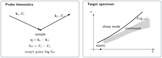
The probe transfers $\hbar\mathbf q=\hbar(\mathbf k_i-\mathbf k_f)$ and $\hbar\omega=E_i-E_f$ to the target. In the resulting $S(\mathbf q,\omega)$ map, elastic order lies at $\omega=0$, a stable collective excitation traces a narrow dispersion, and multi-particle states occupy a continuum. Actual data are multiplied by probe factors and convolved with instrumental resolution.

The two axes resolve different structures:

• a peak position in $\mathbf q$ identifies a dominant wavelength;
• a momentum width of order $\kappa$ often corresponds to a real-space length of order $\kappa^{-1}$;
• a dispersing peak traces an excitation energy $\hbar\omega_{\mathbf q}$;
• an intrinsic frequency width of order $\Gamma$ can correspond to a lifetime of order $\Gamma^{-1}$;
• a continuum boundary records multi-particle kinematics or selection rules;
• redistribution of weight can matter even when peak positions barely move.

The inverse-width statements are scaling estimates, not universal equalities. Line shapes, dimensionality, algebraic prefactors, disorder, and resolution determine the precise conversion.

From Correlations to a Scattering Cross Section

Suppose an incident probe has wavevector $\mathbf k_i$ and energy $E_i$, while the detected probe has $\mathbf k_f$ and $E_f$. This page defines target transfers by

$$\mathbf q = \mathbf k_i-\mathbf k_f, \qquad \hbar\omega = E_i-E_f.$$

Thus $\omega>0$ means the target absorbs energy.

In the first Born or golden-rule regime, a probe that couples linearly to a target operator produces the schematic factorization

$$\frac{d^2\sigma}{ d\Omega\,dE_f } = \mathcal K \, \left| F(\mathbf q) \right|^2 \, \mathcal P \!\left[ S_O(\mathbf q,\omega) \right].$$

Here:

• $\mathcal K$ contains flux and kinematic factors such as $k_f/k_i$;
• $F(\mathbf q)$ is a single-particle, orbital, magnetic, molecular, or Wannier form factor;
• $\mathcal P$ is a scalar or tensor projection set by probe polarization and coupling;
• $S_O$ contains the target’s many-body correlations.

This factorization is not universal beyond weak single-scattering conditions. Multiple scattering, strong final-state interactions, absorption, refraction, detector nonlinearity, and probe-specific vertices can require a more complete forward model.

Neutron Scattering

Neutrons couple both to nuclei and to magnetic moments. Those channels expose different target operators.

Nuclear scattering

Coherent nuclear scattering retains interference among different nuclei and therefore carries collective spatial structure. In the simplest identical-scatterer limit,

$$\frac{d^2\sigma_{\mathrm{coh}}}{ d\Omega\,dE_f } \propto \frac{k_f}{k_i} S_n(\mathbf q,E_i-E_f).$$

Real materials contain isotope- and nuclear-spin-dependent scattering lengths. Their variance produces an incoherent contribution dominated by self correlations. Incoherent scattering is not merely a featureless nuisance: it can measure single-particle motion, but it is not the same collective pair structure factor as the coherent term.

Magnetic scattering

For unpolarized magnetic neutron scattering, a standard schematic form is

$$\begin{aligned} \frac{d^2\sigma_{\mathrm{mag}}}{ d\Omega\,dE_f } \propto{}& \frac{k_f}{k_i} \left| F_{\mathrm{mag}}(\mathbf q) \right|^2 \\ &\times \sum_{\alpha,\beta} \left( \delta_{\alpha\beta} - \widehat q_\alpha \widehat q_\beta \right) S^{\alpha\beta}(\mathbf q,\omega). \end{aligned}$$

The projector removes magnetization parallel to $\mathbf q$: the neutron is sensitive to components transverse to the momentum transfer. The magnetic form factor reflects the spatial distribution of electronic magnetization and usually decreases at large momentum.

Polarized-neutron analysis can separate additional symmetric and antisymmetric tensor combinations. Crystal domains, multiple magnetic ions per cell, $g$-tensor anisotropy, and nuclear–magnetic interference require corresponding structure and polarization factors.

Neutron Scattering owns beam kinematics, instrument architectures, isotope and polarization choices, resolution convolution, normalization, and experimental phonon, magnon, and continuum workflows.

Cold-Atom Probes

Cold-atom platforms realize both frequency-resolved and equal-time measurements without a material crystal.

Two-photon Bragg spectroscopy

Two laser beams with wavevectors $\mathbf k_1,\mathbf k_2$ and frequencies $\omega_1,\omega_2$ create a moving optical potential. The target transfers are

$$\mathbf q = \mathbf k_1-\mathbf k_2, \qquad \omega = \omega_1-\omega_2.$$

In weak driving, the absorption rate at positive $\omega$ is proportional to a density or spin dynamic structure factor, depending on the light coupling. A measured net momentum or energy transfer generally involves the difference between absorption and stimulated emission:

$$S(\mathbf q,\omega) - S(-\mathbf q,-\omega).$$

At low temperature and positive target energy transfer, the reverse term can be strongly suppressed. At finite temperature it must not be silently discarded.

Finite pulse duration broadens frequency resolution. Trap inhomogeneity averages regions with different density and gap scales. Strong pulses cause saturation and nonlinear response. Final-state interactions and optical selection rules can change the operator actually measured.

In particular, a finite-pulse momentum-transfer spectrum in a trapped condensate is a probe response built from the dynamic structure factor, not generally the dynamic structure factor itself. The pulse envelope and inhomogeneous evolution belong in the forward model.

Density snapshots and noise correlations

Quantum gas microscopes and absorption images can estimate equal-time density correlations. Fourier transformation of connected fluctuations produces a static structure factor:

$$\widehat S_n^c(\mathbf q) \propto \left\langle \left| \delta n_{\mathbf q} \right|^2 \right\rangle.$$

Finite imaging resolution multiplies the mode by an optical transfer function. Atom loss, parity projection, finite field of view, trap profiles, and shot-to-shot number fluctuations must be modeled before comparison with a homogeneous theory.

X-Ray and Electron Probes

Elastic and inelastic x-ray scattering primarily couple to charge density, modulated by atomic form factors and photon polarization. Diffraction emphasizes static periodic density, while inelastic x-ray scattering resolves charge dynamics over momentum and energy.

X-Ray Scattering develops the photon kinematics, elastic and resonant amplitudes, absorption corrections, coherent phase retrieval, charge-order workflow, and experimental distinction between nonresonant IXS and RIXS.

Electron energy-loss spectroscopy often reports a loss function such as

$$- \operatorname{Im} \frac{1}{ \epsilon(\mathbf q,\omega) },$$

not a bare structure factor. The loss function, density response, and $S_n(\mathbf q,\omega)$ are related through electrodynamics and fluctuation–dissipation relations under stated conditions, but they are not interchangeable labels.

Plasmons Preview applies this distinction to collective charge modes, including dielectric zeros, loss peaks, and density pole weights.

Raman scattering, resonant x-ray scattering, and optical spectroscopy can couple to stress, spin, orbital, bond, or symmetry-resolved composite operators. “Scattering measures $S$” is only meaningful after the operator and vertex are specified.

Order, Criticality, and Peak Scaling

The full phase criterion and its finite-size caveats are developed in Long-Range Order. This section records how those regimes appear in the present Fourier convention.

Let $O_j$ have ordering wavevector $\mathbf Q$. If a full equal-time correlator approaches a nonzero plateau,

$$\left\langle O_iO_j \right\rangle \longrightarrow m^2 e^{i\mathbf Q\cdot (\mathbf r_i-\mathbf r_j)},$$

then

$$S_O(\mathbf Q) \sim L m^2.$$

The peak height is extensive under the $1/L$ convention. Equivalently,

$$\frac{ S_O(\mathbf Q) }{L} \longrightarrow m^2$$

after the correct thermodynamic and phase-selection limits.

Short-range connected correlations produce a peak whose height is controlled by a correlation volume rather than the whole system. Landau–Ginzburg Theory Preview derives the Gaussian Lorentzian peak and its width $\xi^{-1}$; the normalization and experimental qualifications remain here. Near a critical point, if

$$C_O^c(r) \sim r^{-2\Delta_O},$$

then a finite system of linear size $\ell$ can show

$$S_O^c(\mathbf Q) \sim \ell^{d-2\Delta_O}$$

when the infrared integral diverges with size. Marginal cases can carry logarithms.

Critical Exponents and Scaling owns the relation among this peak power, $\eta$, $\nu$, and $\gamma$, together with finite-size corrections and collapse practice.

Peak height alone is insufficient. Reliable phase inference combines:

• height scaling with $L$ or $\ell$;
• peak-width scaling and a correlation-length estimator;
• the full versus connected convention;
• boundary and aspect-ratio dependence;
• tensor and domain projections;
• an order-parameter or Binder-style cross-check.

Example: Uncorrelated Uniform Particles

For independent distinguishable particles, or a classical ideal gas, uniformly distributed in a periodic volume and at a nonzero allowed momentum,

$$\left\langle e^{-i\mathbf q\cdot\mathbf r_j} \right\rangle = 0.$$

Then

$$\begin{aligned} S_n(\mathbf q) &= \frac{1}{N} \sum_{i,j} \left\langle e^{-i\mathbf q\cdot (\mathbf r_i-\mathbf r_j)} \right\rangle \\ &= \frac{1}{N} \sum_i 1 \\ &= 1. \end{aligned}$$

The result is the self term. Bose or Fermi exchange, interactions, a trap, or a global constraint changes the cross terms even when no classical pair force is present.

At $\mathbf q=\mathbf 0$, the argument fails because every phase equals one. The full fixed-$N$ value is $N$, whereas the connected value is zero.

Example: Néel Order and Phase Selection

Consider an even one-dimensional chain with

$$\left\langle s_j^z \right\rangle_+ = m(-1)^j, \qquad \mathbf Q = \frac{\pi}{a}.$$

In the selected product pattern,

$$\left\langle s_{\mathbf Q}^z \right\rangle_+ = Lm.$$

Therefore

$$S_{\mathrm{full}}^{zz}(\mathbf Q) = Lm^2,$$

while the connected structure factor of the exact product pattern vanishes because there are no fluctuations about its local means.

An equal mixture of the two translated Néel patterns has

$$\left\langle s_j^z \right\rangle_{\mathrm{mix}} = 0$$

but retains

$$S_{\mathrm{mix}}^{zz}(\mathbf Q) = S_{\mathrm{mix},c}^{zz}(\mathbf Q) = Lm^2.$$

The same sharp static peak can therefore coexist with different one-point functions and different clustering properties. Structure-factor data alone do not determine whether the state is a selected phase, a symmetric mixture, or a coherent finite-volume state.

Example: Antiferromagnetic Spin Dimer

For two spin-$1/2$ sites separated by $a$ in a singlet,

$$\left\langle \mathbf s_1^2 \right\rangle = \left\langle \mathbf s_2^2 \right\rangle = \frac{3}{4},$$

and

$$\left\langle \mathbf s_1\cdot\mathbf s_2 \right\rangle = - \frac{3}{4}.$$

With $L=2$,

$$\begin{aligned} S(\mathbf q) &= \frac{1}{2} \sum_{i,j} e^{-i\mathbf q\cdot (\mathbf r_i-\mathbf r_j)} \left\langle \mathbf s_i\cdot\mathbf s_j \right\rangle \\ &= \frac{3}{4} \left[ 1-\cos(qa) \right]. \end{aligned}$$

Thus

$$S(0) = 0, \qquad S(\pi/a) = \frac{3}{2}.$$

The zero-momentum cancellation expresses total-spin singlet character. The antiferromagnetic momentum maximizes the contrast between opposite spins. For the Heisenberg dimer, the dynamic spin structure factor places the corresponding inelastic weight at the singlet–triplet gap.

Modes, Continua, and Spectral Weight

A sharp quasiparticle contribution has the form

$$S_O(\mathbf q,\omega) \supset Z_O(\mathbf q) \delta\!\left( \omega-\omega_{\mathbf q} \right).$$

The residue

$$Z_O(\mathbf q)$$

depends on the operator. A real excitation can be absent from a chosen structure factor because symmetry makes its matrix element vanish.

Interactions can broaden a mode or move weight into a continuum:

$$S_O = S_O^{\mathrm{mode}} + S_O^{\mathrm{cont}}.$$

The integrated weight must still satisfy exact moments. Calling a broad feature “a particle” without checking size, resolution, thresholds, and sum rules can overstate the evidence. Phonons as Many-Body Excitations derives the displacement matrix element, polarization factor, and creation–annihilation weights behind the harmonic one-phonon peak.

Particle–Hole Excitations derives the occupied-to-empty promotion, Pauli-constrained continuum boundaries, and the independent density response whose absorptive part supplies a canonical fermionic continuum.

Bogoliubov Quasiparticles shows how particle–hole amplitudes combine into density, spin, current, and pair-channel coherence factors before they become the operator-dependent weight $Z_O$.

The Heisenberg Model provides a standard contrast: higher-dimensional ordered magnets can show sharp magnons, while a one-dimensional spin-$1/2$ antiferromagnet has prominent spinon continua. Magnons derives the transverse one-magnon matrix elements, sublattice coherence factors, and longitudinal multi-magnon onset. Goldstone Modes in Many-Body Systems explains when a soft pole is enforced by broken symmetry and how its finite-size and low-momentum scaling should be tested.

First Moment and the Density f-Sum

The first angular-frequency moment is

$$m_1(\mathbf q) = \int d\omega\, \omega S_O(\mathbf q,\omega).$$

For the density channel of a homogeneous continuum system in equilibrium,

$$\begin{aligned} m_{1,n}(\mathbf q) ={}& \frac{1}{ 2\hbar N } \\ &\times \left\langle \left[ \rho_{\mathbf q}, \left[ H, \rho_{-\mathbf q} \right] \right] \right\rangle. \end{aligned}$$

For nonrelativistic particles of mass $m$ with position-dependent interactions,

$$\int d\omega\, \omega S_n(\mathbf q,\omega) = \frac{ \hbar q^2 }{ 2m }.$$

This is the per-particle density $f$-sum rule in the present angular-frequency convention. Lattices, multiple species, nonlocal interactions, spin–orbit coupling, and projected bands modify the commutator result.

At zero temperature, if one sharp mode exhausts the density weight,

$$S_n(\mathbf q,\omega) = S_n(\mathbf q) \delta\!\left( \omega-\omega_{\mathbf q} \right),$$

then

$$\hbar\omega_{\mathbf q} = \frac{ \hbar^2q^2 }{ 2mS_n(\mathbf q) }.$$

This is the single-mode or Feynman relation under a strong assumption. With a continuum, the ratio $m_1/m_0$ is a weighted mean frequency rather than the energy of every excitation.

Sum Rules owns the systematic moment derivations; the equations here serve as normalization and interpretation checks.

Compressibility and Response Boundary

In a homogeneous equilibrium fluid at nonzero temperature, an appropriate thermodynamic limit gives

$$\lim_{\mathbf q\to\mathbf 0} S_n^c(\mathbf q) = n k_{\mathrm B}T \kappa_T,$$

where $\kappa_T$ is the isothermal compressibility. The exactly conserved $\mathbf q=0$ mode in a canonical finite system can still vanish.

The dynamic structure factor is related to the dissipative density response by a fluctuation–dissipation theorem. That relation includes thermal factors and convention-dependent signs; it does not make $S$ itself causal. Kubo Formula owns retarded response, while Fluctuations and Susceptibilities owns thermodynamic fluctuation scaling.

Numerical Evaluation

Equal-time configurations

For periodic lattice samples,

$$S_O^c(\mathbf q) = \frac{1}{L} \left\langle \left| \delta O_{\mathbf q} \right|^2 \right\rangle$$

can be accumulated with a discrete Fourier transform. Subtract local profiles before averaging in inhomogeneous systems. Check positivity, the onsite momentum sum, symmetry-related momenta, and exact conserved modes.

Exact diagonalization

The Lehmann sum produces exact finite-size delta lines. Artificial broadening is useful for plotting but must preserve integrated weight. A chosen Lorentzian width is not a lifetime.

Real-time tensor networks

Compute

$$C_O(\mathbf q,t) = \frac{1}{L} \left\langle O_{\mathbf q}(t) O_{-\mathbf q}(0) \right\rangle$$

and Fourier transform a finite time interval. Entanglement growth limits $t_{\max}$; the resulting frequency resolution is of order $1/t_{\max}$. Window functions trade ringing against broadening and can alter peak height.

Imaginary-time methods

For

$$0\leq\tau\leq\beta\hbar,$$

the imaginary-time density correlator has the spectral form

$$F(\mathbf q,\tau) = \int d\omega\, e^{-\omega\tau} S_n(\mathbf q,\omega).$$

Recovering real-frequency structure from noisy imaginary-time data is an ill-conditioned inverse problem. Maximum entropy, stochastic continuation, sparse models, or neural methods introduce assumptions; agreement with moments and synthetic benchmarks is essential.

Correction-vector and Krylov methods

Frequency-domain resolvents can target selected $\omega$ directly, while Krylov propagation resolves finite-time dynamics. Linear-system tolerance, boundary reflections, bond dimension, and broadening all affect the inferred line shape.

Experimental Forward Model

Measured counts are better represented schematically by

$$\begin{aligned} I_{\mathrm{meas}}(\mathbf q,\omega) ={}& \int d^d q'\,d\omega'\, R( \mathbf q-\mathbf q', \omega-\omega' ) \\ &\times M(\mathbf q',\omega') + B(\mathbf q,\omega), \end{aligned}$$

where:

• $M$ contains the cross section, structure factor, form factors, and polarization terms;
• $R$ is the multidimensional instrumental resolution;
• $B$ is background.

Deconvolution can be unstable. It is often more reliable to convolve a theoretical model with $R$ and fit it in measurement space.

Important corrections include:

• incident flux and detector efficiency;
• absorption and sample self-shielding;
• multiple scattering;
• empty-container, substrate, and environmental backgrounds;
• form-factor and Debye–Waller corrections;
• polarization leakage and domain populations;
• finite energy and momentum acceptance;
• powder or angular averaging;
• absolute intensity calibration;
• detailed-balance consistency;
• uncertainty covariance across bins.

Validation Checklist

1. State whether the operator mode uses $e^{-i\mathbf q\cdot\mathbf r}$ or the opposite sign.
2. State every factor of $L$, $N$, $2\pi$, and $\hbar$.
3. Distinguish angular frequency from energy transfer.
4. Check $O_{\mathbf q}^{\dagger}=O_{-\mathbf q}$ for the chosen channel.
5. Verify scalar positivity or tensor positive semidefiniteness.
6. Integrate $S(\mathbf q,\omega)$ and recover the static structure factor.
7. Enforce detailed balance in a thermal calculation.
8. Separate exact elastic, quasielastic, and inelastic weight.
9. Check onsite, total-charge, total-spin, and first-moment sum rules.
10. Compare peak height and width across system sizes.
11. Include form factors, polarization projectors, and resolution before comparing with counts.
12. Test the extraction pipeline on synthetic spectra with known lines and continua.

Common Mistakes

• Calling a real-space correlation function a structure factor before Fourier transformation.
• Mixing full and connected definitions at an ordering wavevector.
• Treating every zero-frequency contribution as a removable one-point product.
• Comparing per-site and extensive normalizations as if they were equal.
• Forgetting the $1/\hbar$ Jacobian between $S(\mathbf q,\omega)$ and $S(\mathbf q,E)$.
• Reversing the target energy-transfer sign when switching probe conventions.
• Assuming $S(\mathbf q,\omega)$ is a retarded response function.
• Expecting negative-frequency weight to vanish at finite temperature.
• Interpreting a finite plotting width as an intrinsic lifetime.
• Inferring long-range order from one finite-size peak without scaling.
• Ignoring the self term in the density structure factor.
• Evaluating $\mathbf q=0$ before the thermodynamic limit without stating the ensemble.
• Treating a magnetic neutron cross section as an unprojected spin trace.
• Dividing out a form factor without propagating its uncertainty.
• Calling incoherent neutron scattering featureless background.
• Equating an energy-integrated finite-window intensity with the full static moment.
• Analytically continuing imaginary-time data without moment and resolution checks.
• Comparing experiment and theory before convolving with instrumental resolution.

Reliable Workflow

1. Choose the target operator and tensor component.
2. Fix the spatial and temporal Fourier conventions.
3. Decide whether full, connected, elastic-subtracted, or symmetrized data are needed.
4. Derive the Lehmann representation and support for the chosen sign convention.
5. Check static, detailed-balance, and commutator moments.
6. Identify the allowed finite-size momenta and boundary effects.
7. Separate Bragg peaks, quasielastic weight, modes, and continua.
8. Match the probe coupling to density, spin, current, bond, or pair operators.
9. Build form factors, polarization, kinematics, and resolution into a forward model.
10. Fit several sizes, windows, and background models.
11. Propagate correlated uncertainty and calibration errors.
12. Report conventions next to every published spectrum.

Exercises

Exercise 1: Positivity and the momentum sum

Show that

$$S_O^c(\mathbf q) = \frac{1}{L} \left\langle \delta O_{\mathbf q} \delta O_{\mathbf q}^{\dagger} \right\rangle \geq 0.$$

For a translation-invariant periodic lattice, also prove

$$\frac{1}{L} \sum_{\mathbf q} S_O^c(\mathbf q) = \left\langle (\delta O_j)^2 \right\rangle.$$

Solution

For any vector $\lvert\psi\rangle$,

$$\left\langle \psi \middle| \delta O_{\mathbf q} \delta O_{\mathbf q}^{\dagger} \middle| \psi \right\rangle = \left\| \delta O_{\mathbf q}^{\dagger} \lvert\psi\rangle \right\|^2 \geq 0.$$

A density operator is a positive mixture of such vectors, so its expectation remains nonnegative.

Translation invariance gives

$$S_O^c(\mathbf q) = \sum_{\mathbf r} e^{-i\mathbf q\cdot\mathbf r} C_O^c(\mathbf r).$$

Therefore

$$\begin{aligned} \frac{1}{L} \sum_{\mathbf q} S_O^c(\mathbf q) &= \sum_{\mathbf r} C_O^c(\mathbf r) \left[ \frac{1}{L} \sum_{\mathbf q} e^{-i\mathbf q\cdot\mathbf r} \right] \\ &= C_O^c(\mathbf 0) \\ &= \left\langle (\delta O_j)^2 \right\rangle. \end{aligned}$$

The bracket is the discrete reciprocal-lattice delta function.

Exercise 2: Zeroth moment

Starting from

$$\begin{aligned} S_O(\mathbf q,\omega) ={}& \frac{1}{L} \sum_{n,m} p_n \left| \langle m| O_{-\mathbf q} |n\rangle \right|^2 \\ &\times \delta\!\left( \omega- \frac{E_m-E_n}{\hbar} \right), \end{aligned}$$

show that its integral equals $S_O(\mathbf q)$.

Solution

Integrating the delta function gives

$$\int d\omega\, S_O(\mathbf q,\omega) = \frac{1}{L} \sum_{n,m} p_n \left| \langle m| O_{-\mathbf q} |n\rangle \right|^2.$$

Use completeness:

$$\begin{aligned} \sum_m \left| \langle m| O_{-\mathbf q} |n\rangle \right|^2 &= \langle n| O_{\mathbf q} O_{-\mathbf q} |n\rangle. \end{aligned}$$

Then

$$\int d\omega\, S_O(\mathbf q,\omega) = \frac{1}{L} \operatorname{Tr} \left( \rho O_{\mathbf q} O_{-\mathbf q} \right) = S_O(\mathbf q).$$

Exercise 3: Detailed balance

For a thermal state, derive

$$S_O(-\mathbf q,-\omega) = e^{-\beta\hbar\omega} S_O(\mathbf q,\omega).$$

Solution

Write

$$\begin{aligned} S_O(-\mathbf q,-\omega) ={}& \frac{1}{L} \sum_{n,m} p_n \left| \langle m| O_{\mathbf q} |n\rangle \right|^2 \\ &\times \delta\!\left( -\omega- \frac{E_m-E_n}{\hbar} \right). \end{aligned}$$

Exchange $n$ and $m$. On the delta-function support,

$$E_m-E_n = \hbar\omega.$$

The Boltzmann weights obey

$$p_m = p_n e^{-\beta(E_m-E_n)} = p_n e^{-\beta\hbar\omega}.$$

The exchanged matrix element is the one appearing in $S_O(\mathbf q,\omega)$, so the stated factor follows.

Exercise 4: Independent-particle baseline

For $N$ independent particles uniformly distributed in a periodic box, show that

$$S_n(\mathbf q) = 1$$

for every nonzero allowed momentum. Why does the same argument fail at $\mathbf q=0$?

Solution

Expand

$$S_n(\mathbf q) = \frac{1}{N} \sum_{i,j} \left\langle e^{-i\mathbf q\cdot\mathbf r_i} e^{i\mathbf q\cdot\mathbf r_j} \right\rangle.$$

For $i=j$, every term is one. For $i\neq j$, independence factorizes the average:

$$\left\langle e^{-i\mathbf q\cdot\mathbf r_i} \right\rangle \left\langle e^{i\mathbf q\cdot\mathbf r_j} \right\rangle.$$

Uniformity makes either factor zero at a nonzero allowed reciprocal momentum. Thus only the $N$ self terms survive and $S_n=1$.

At $\mathbf q=0$, every phase is one, so all $N^2$ terms survive. The full fixed-number value is $N$; the connected value is zero because $\delta N=0$.

Exercise 5: Selected and mixed Néel states

Let $s_j^z=m(-1)^j$ on an even chain. Compute the full and connected structure factors at $Q=\pi/a$ in:

1. one selected product pattern;
2. an equal mixture of the two translated patterns.

Solution

In either selected pattern,

$$s_Q^z = \sum_j e^{-i\pi j} s_j^z = \pm Lm.$$

Hence

$$S_{\mathrm{full}}^{zz}(Q) = \frac{1}{L} \left| \langle s_Q^z\rangle \right|^2 = Lm^2.$$

The local variables have no fluctuations in the product pattern, so

$$S_c^{zz}(Q) = 0.$$

In the equal mixture,

$$\langle s_j^z\rangle_{\mathrm{mix}} = 0,$$

but both components have

$$\left| s_Q^z \right|^2 = L^2m^2.$$

Therefore

$$S_{\mathrm{full}}^{zz}(Q) = S_c^{zz}(Q) = Lm^2.$$

The mixture retains the ordered global label and fails cluster decomposition.

Exercise 6: Spin-dimer structure factor

For a spin-$1/2$ singlet on sites at $0$ and $a$, derive

$$S(q) = \frac{3}{4} \left[ 1-\cos(qa) \right].$$

Check $q=0$ and $q=\pi/a$.

Solution

The onsite terms contribute

$$\frac{1}{2} \left( \frac{3}{4} + \frac{3}{4} \right) = \frac{3}{4}.$$

The two cross terms contribute

$$\begin{aligned} &\frac{1}{2} \left[ e^{iqa} \left( -\frac{3}{4} \right) + e^{-iqa} \left( -\frac{3}{4} \right) \right] \\ &= - \frac{3}{4} \cos(qa). \end{aligned}$$

Adding onsite and cross terms gives

$$S(q) = \frac{3}{4} \left[ 1-\cos(qa) \right].$$

Thus

$$S(0) = 0,$$

as required for a total-spin singlet, while

$$S(\pi/a) = \frac{3}{2}.$$

Exercise 7: Frequency and energy conventions

Suppose $S_\omega(\mathbf q,\omega)$ satisfies

$$\int d\omega\, S_\omega(\mathbf q,\omega) = S(\mathbf q).$$

Find $S_E(\mathbf q,E)$ such that

$$\int dE\, S_E(\mathbf q,E) = S(\mathbf q),$$

with $E=\hbar\omega$.

Solution

Because

$$dE = \hbar\,d\omega,$$

the two integrands must satisfy

$$S_E(\mathbf q,E)\,dE = S_\omega(\mathbf q,\omega)\,d\omega.$$

Therefore

$$S_E(\mathbf q,E) = \frac{1}{\hbar} S_\omega\!\left( \mathbf q, \frac{E}{\hbar} \right).$$

The factor $1/\hbar$ is required both by normalization and by units.

Exercise 8: Single-mode estimate

At zero temperature, assume the density spectrum is exhausted by

$$S_n(\mathbf q,\omega) = S_n(\mathbf q) \delta( \omega-\omega_{\mathbf q} ).$$

Use the $f$-sum rule to derive the single-mode relation. What changes if a continuum carries part of the weight?

Solution

The first moment of the assumed spectrum is

$$\int d\omega\, \omega S_n(\mathbf q,\omega) = \omega_{\mathbf q} S_n(\mathbf q).$$

The density $f$-sum rule gives

$$\omega_{\mathbf q} S_n(\mathbf q) = \frac{ \hbar q^2 }{ 2m }.$$

Hence

$$\hbar\omega_{\mathbf q} = \frac{ \hbar^2q^2 }{ 2mS_n(\mathbf q) }.$$

If a continuum carries weight, then

$$\frac{m_1}{m_0}$$

is the spectral mean frequency. It need not equal the position of a sharp mode, a threshold, or every excitation energy.

Cross-Links

• How Quantum Matter Is Measured situates structure factors inside a scattering forward model with form factors, polarization, depth, resolution, background, and sample-volume effects.
• Correlation Function Definitions — static and dynamic structure-factor normalization in the shared correlation dictionary.
• Correlation Functions Overview — map of real-space, temporal, ordered, and response objects.
• Equal-Time Correlations — canonical static operator channels and contact terms.
• Time-Dependent Correlations — Lehmann spectra, detailed balance, dephasing, and finite-time transforms.
• Connected Correlation Functions — subtraction, clustering, phase mixtures, and correlation lengths.
• Long-Range Order — real-space plateaus and extensive versus subextensive ordering peaks.
• Antiferromagnetism — magnetic propagation vectors, transverse neutron factors, Bragg peaks, domains, and finite-size Néel diagnostics.
• Spin Waves and Magnons in Materials — applies dynamic spin structure factors to magnetic form factors, polarization projectors, mode eigenvectors, resolution, and linewidth fitting.
• Green Functions in Many-Body QM — single-particle addition and removal spectra.
• Retarded and Advanced Response — causal support, response spectral density, and analytic checks.
• Susceptibilities — named response channels, units, and measurable limits.
• Spectral Functions — exact lines, continua, linewidths, spectral weight, and measured intensity.
• Fluctuation–Dissipation Theorem — detailed balance and the response encoded by scattering spectra.
• Sum Rules — exact zeroth and energy-weighted constraints, including the density $f$-sum.
• Kubo Formula — retarded response and source conventions.
• Fluctuations and Susceptibilities — integrated connected correlations and thermodynamic response.
• Heisenberg Model — spin structure factors, order, magnons, and continua.
• Hubbard Model — charge, spin, and pairing channels.
• Random Phase Approximation — collective density response and screened poles.
• Scattering Experiment — counts, exposure, acceptance, efficiency, and detector response.
• Inelastic Scattering Preview — channel kinematics and cross sections.
• Fourier Transform Conventions — transform signs, measures, and variable changes.

References

1. L. Van Hove, “Correlations in Space and Time and Born Approximation Scattering in Systems of Interacting Particles”, Physical Review 95, 249–262 (1954).
2. L. Van Hove, “Time-Dependent Correlations between Spins and Neutron Scattering in Ferromagnetic Crystals”, Physical Review 95, 1374–1384 (1954).
3. J. Stenger, S. Inouye, A. P. Chikkatur, D. M. Stamper-Kurn, D. E. Pritchard, and W. Ketterle, “Bragg Spectroscopy of a Bose–Einstein Condensate”, Physical Review Letters 82, 4569–4573 (1999).
4. R. P. Feynman, “Atomic Theory of the Two-Fluid Model of Liquid Helium”, Physical Review 94, 262–277 (1954).
5. P. C. Hohenberg and W. F. Brinkman, “Sum Rules for the Frequency Spectrum of Linear Magnetic Chains”, Physical Review B 10, 128–131 (1974).
6. P. B. Blakie, R. J. Ballagh, and C. W. Gardiner, “Theory of Coherent Bragg Spectroscopy of a Trapped Bose–Einstein Condensate”, Physical Review A 65, 033602 (2002).
7. G. L. Squires, Introduction to the Theory of Thermal Neutron Scattering, 3rd ed., Cambridge University Press (2012).
8. S. W. Lovesey, Theory of Neutron Scattering from Condensed Matter, Clarendon Press (1984).
9. A. L. Fetter and J. D. Walecka, Quantum Theory of Many-Particle Systems, Dover (2003).
10. P. Nozières and D. Pines, The Theory of Quantum Liquids, Westview Press (1999).
11. L. Pitaevskii and S. Stringari, Bose–Einstein Condensation and Superfluidity, Oxford University Press (2016).