Random Phase Approximation

The random phase approximation (RPA) describes the collective linear response of an interacting many-body system by letting a simple reference system respond self-consistently to the field induced by its own density fluctuation. In its elementary density form, RPA replaces the exact irreducible polarization by the independent-particle polarization and sums the resulting feedback to all orders.

The central structure is

$$\text{external field} \longrightarrow \text{density fluctuation} \longrightarrow \text{induced field} \longrightarrow \text{density fluctuation}.$$

Although each polarization step is computed from noninteracting particles, the infinite feedback chain can produce behavior absent from every finite perturbative order: screened interactions, collective poles, and plasma oscillations.

RPA is not a claim that phases are literally random, and it is not a generic synonym for “include fluctuations.” It is a specific closure of a response or particle–hole problem. Its reliability depends on the interaction range, density, reference state, channel, dimension, frequency, and observable.

Canonical Scope

This page is the canonical home for:

• the independent-particle density polarization;
• the Lindhard polarization as the independent-particle input;
• the self-consistent-field derivation of RPA;
• the equivalent bubble-chain or ring resummation;
• dielectric screening and the screened interaction;
• Thomas–Fermi screening as the static long-wavelength limit;
• the RPA derivation of collective poles and the long-wavelength plasmon scale;
• how the particle–hole continuum produces Landau damping in RPA;
• direct RPA, RPA with exchange, and time-dependent Hartree–Fock terminology;
• finite-basis particle–hole RPA;
• ring correlation energy;
• conservation laws, sum rules, validity conditions, and failure modes.

Kubo Formula owns exact first-order response to an external source, including signs, contact terms, order of limits, and Lehmann representations. This page instead owns one approximation for evaluating an interacting response. Density Operators and Current Operators owns the operators and continuity equations. Collective Modes owns the general response-eigenmode, polarization, hybridization, and damping language. Particle–Hole Excitations owns the generic excitation concept, hole quantum numbers, phase-space support, and continuum kinematics; the derivation below retains only the homogeneous parabolic-band boundaries needed to diagnose RPA damping. Plasmons Preview owns the general collective-charge interpretation, while this page owns its emergence from the RPA dielectric denominator. Detailed plasmon phenomenology in particular materials belongs in Quantum Matter.

Why the Name Is Ambiguous

Several related approximations are called RPA:

1. Direct density RPA uses a noninteracting polarization bubble and a direct density interaction.
2. Time-dependent Hartree RPA is the same closure obtained by linearizing a time-dependent Hartree equation.
3. RPA with exchange or time-dependent Hartree–Fock includes exchange in the particle–hole kernel.
4. Finite-basis RPA solves a forward-and-backward particle–hole eigenvalue problem around a mean-field reference.
5. Ring RPA sums ring diagrams in response functions or the correlation energy.
6. Density-functional RPA uses a chosen independent-particle response and the bare Coulomb kernel in an adiabatic-connection energy formula.

These forms share a small-oscillation or repeated particle–hole structure, but they are not numerically identical. Every use of “RPA” should state:

• the reference propagator or orbitals;
• the interaction kernel;
• whether exchange or another vertex kernel is included;
• whether the target is response, excitation energies, or ground-state correlation energy.

This page derives direct density RPA first and then maps the main variants around it.

Source and Sign Conventions

Let a potential energy $U_{\mathrm{ext}}$ couple to the number density:

$$\delta K_{\mathrm{ext}}(t) = \int d^d r\, U_{\mathrm{ext}}(\mathbf r,t) n(\mathbf r).$$

In momentum and frequency space, define the retarded polarization by

$$\delta n(\mathbf q,\omega) = \Pi^R(\mathbf q,\omega) U_{\mathrm{ext}}(\mathbf q,\omega).$$

A positive static potential energy repels particles, so a stable fermion gas has

$$\Pi^R(\mathbf q\to0,0) < 0.$$

The Kubo Formula uses a local chemical-potential source,

$$\delta K_{\mathrm{ext}} = - \int d^d r\, \delta\mu_{\mathrm{ext}}n,$$

and defines

$$\delta n = \chi_{nn}^R \delta\mu_{\mathrm{ext}}.$$

Because

$$U_{\mathrm{ext}} = -\delta\mu_{\mathrm{ext}},$$

the two conventions are related by

$$\Pi^R = -\chi_{nn}^R.$$

This page writes screening formulas with $\Pi$, for which the familiar dielectric denominator is $1-v\Pi$. When translating to the site’s chemical-potential susceptibility, replace $\Pi$ by $-\chi$.

Density–Density Interaction

Consider a translationally invariant reference Hamiltonian

$$K_0 = \sum_{\mathbf k,\sigma} \xi_{\mathbf k} c_{\mathbf k\sigma}^\dagger c_{\mathbf k\sigma}.$$

Define the Fourier density

$$n_{\mathbf q} = \sum_{\mathbf k,\sigma} c_{\mathbf k\sigma}^\dagger c_{\mathbf k+\mathbf q,\sigma}.$$

A direct density interaction can be written

$$K_{\mathrm{int}} = \frac{1}{2\mathcal V} \sum_{\mathbf q} v_{\mathbf q} : n_{\mathbf q} n_{-\mathbf q} :.$$

The normal-ordering convention and treatment of $\mathbf q=0$ must be stated. For a Coulomb electron gas, a uniform positive background cancels the divergent uniform Hartree term. One usually excludes $\mathbf q=0$ from the fluctuating interaction and imposes overall neutrality.

The scalar derivation below assumes one density channel and a real even kernel,

$$v_{\mathbf q} = v_{-\mathbf q}.$$

Multicomponent, spin, orbital, and sublattice systems require matrices in the corresponding channel space.

Independent-Particle Polarization

The noninteracting response of $K_0$ is the Lindhard polarization:

$$\begin{aligned} \Pi_0^R(\mathbf q,\omega) ={}& \frac{1}{\mathcal V} \sum_{\mathbf k,\sigma} \frac{ f(\xi_{\mathbf k}) - f(\xi_{\mathbf k+\mathbf q}) }{ \hbar\omega + \xi_{\mathbf k} - \xi_{\mathbf k+\mathbf q} + i0^+ }. \end{aligned}$$

The spin sum is explicit. If a spin degeneracy factor is pulled out, it must not be inserted a second time in the density of states.

This formula is exact for the independent reference system. It is not yet RPA.

Origin of the numerator

The density operator moves one fermion from $\mathbf k$ to $\mathbf k+\mathbf q$. The occupation difference

$$f(\xi_{\mathbf k}) - f(\xi_{\mathbf k+\mathbf q})$$

implements Pauli blocking. At zero temperature and positive frequency, an absorptive process requires:

$$\xi_{\mathbf k}<0, \qquad \xi_{\mathbf k+\mathbf q}>0.$$

The initial state is occupied and the final state is empty.

Origin of the denominator

The energy transfer for one particle–hole excitation is

$$\Delta\xi_{\mathbf k,\mathbf q} = \xi_{\mathbf k+\mathbf q} - \xi_{\mathbf k}.$$

The retarded denominator has a pole when

$$\hbar\omega = \Delta\xi_{\mathbf k,\mathbf q},$$

with $+i0^+$ selecting causal boundary conditions.

Real and imaginary parts

Using

$$\frac{1}{x+i0^+} = \mathcal P\frac{1}{x} - i\pi\delta(x),$$

one obtains

$$\begin{aligned} \operatorname{Im} \Pi_0^R(\mathbf q,\omega) ={}& - \frac{\pi}{\mathcal V} \sum_{\mathbf k,\sigma} \left[ f(\xi_{\mathbf k}) - f(\xi_{\mathbf k+\mathbf q}) \right] \\ &\times \delta \left( \hbar\omega + \xi_{\mathbf k} - \xi_{\mathbf k+\mathbf q} \right). \end{aligned}$$

For $\omega>0$, the absorptive part is nonpositive in this convention. The real and imaginary parts are linked by causality through dispersion relations.

Static and Uniform Limits

At exactly $\mathbf q=0$,

$$n_{\mathbf q=0} = \widehat N.$$

If particle number is conserved, then for nonzero frequency

$$\Pi_0^R(\mathbf 0,\omega) = 0.$$

The thermodynamic static limit is different. Taking $\omega=0$ and then $\mathbf q\to0$ gives

$$\lim_{\mathbf q\to0} \Pi_0^R(\mathbf q,0) = - \frac{\partial n}{\partial\mu}.$$

At zero temperature,

$$\frac{\partial n}{\partial\mu} = \nu_{\mathrm{tot}}(E_{\mathrm F}),$$

where $\nu_{\mathrm{tot}}$ includes all internal degeneracies.

Thus

$$\Pi_0^R(\mathbf q\to0,0) = -\nu_{\mathrm{tot}}(E_{\mathrm F}).$$

The static and uniform limits encode different protocols. RPA does not remove this order-of-limits issue.

Particle–Hole Continuum

The set of allowed independent particle–hole energies forms a continuum in the thermodynamic limit. For a three-dimensional parabolic band at zero temperature,

$$\epsilon_{\mathbf k} = \frac{\hbar^2k^2}{2m},$$

the positive-frequency continuum lies within

$$\omega_{\min}(q) \le \omega \le \omega_{\max}(q),$$

where

$$\omega_{\min}(q) = \max \left( 0, \frac{\hbar q^2}{2m} - v_{\mathrm F}q \right),$$

and

$$\omega_{\max}(q) = \frac{\hbar q^2}{2m} + v_{\mathrm F}q.$$

Inside this region,

$$\operatorname{Im}\Pi_0^R \ne 0.$$

An excitation can decay into particle–hole pairs there. Outside the continuum, the independent response is purely reactive in the ideal zero-temperature model.

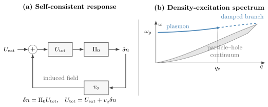
Left: direct RPA closes the loop $U_{\mathrm{tot}}\to\Pi_0\to\delta n\to v\delta n$. Right: a zero of $\varepsilon_{\mathrm{RPA}}(q,\omega)$ gives a collective branch. Outside the particle–hole continuum the ideal mode is sharp; after entering the continuum it acquires Landau damping.

Self-Consistent-Field Derivation

The total potential energy seen by the particles is

$$U_{\mathrm{tot}} = U_{\mathrm{ext}} + U_{\mathrm{ind}}.$$

In direct Hartree response,

$$U_{\mathrm{ind}}(\mathbf q,\omega) = v_{\mathbf q} \delta n(\mathbf q,\omega).$$

Approximate the response to the total field by the independent-particle polarization:

$$\delta n = \Pi_0^R U_{\mathrm{tot}}.$$

Substitution gives

$$\delta n = \Pi_0^R \left( U_{\mathrm{ext}} + v_{\mathbf q}\delta n \right).$$

Move the feedback term to the left:

$$\left( 1 - v_{\mathbf q}\Pi_0^R \right) \delta n = \Pi_0^R U_{\mathrm{ext}}.$$

Therefore

$$\Pi_{\mathrm{RPA}}^R(\mathbf q,\omega) = \frac{ \Pi_0^R(\mathbf q,\omega) }{ 1 - v_{\mathbf q} \Pi_0^R(\mathbf q,\omega) }.$$

This is the scalar direct-RPA density response.

Physical sign check

For a repulsive interaction,

$$v_{\mathbf q}>0.$$

In the static limit,

$$\Pi_0^R<0.$$

Hence

$$1-v_{\mathbf q}\Pi_0^R > 1.$$

The magnitude of the static density response is reduced: the induced Hartree field opposes the external perturbation. If a convention gives static antiscreening for a simple repulsive Coulomb gas, its signs should be audited.

Chemical-potential susceptibility form

Using

$$\chi_0^R = -\Pi_0^R,$$

the same result is

$$\chi_{\mathrm{RPA}}^R = \frac{ \chi_0^R }{ 1 + v_{\mathbf q}\chi_0^R }.$$

Both formulas describe the same physics. Mixing the numerator convention from one with the denominator convention from the other produces a false pole.

Dielectric Function

Define the longitudinal RPA dielectric function by

$$\varepsilon_{\mathrm{RPA}}(\mathbf q,\omega) = 1 - v_{\mathbf q} \Pi_0^R(\mathbf q,\omega).$$

The total and external potential energies obey

$$U_{\mathrm{tot}} = \varepsilon_{\mathrm{RPA}}^{-1} U_{\mathrm{ext}}.$$

The screened interaction is

$$W_{\mathrm{RPA}}^R(\mathbf q,\omega) = \frac{ v_{\mathbf q} }{ \varepsilon_{\mathrm{RPA}}(\mathbf q,\omega) } = \frac{ v_{\mathbf q} }{ 1-v_{\mathbf q}\Pi_0^R }.$$

The identities

$$\Pi_{\mathrm{RPA}}^R = \Pi_0^R \varepsilon_{\mathrm{RPA}}^{-1}$$

and

$$W_{\mathrm{RPA}}^R = v + v\Pi_{\mathrm{RPA}}^Rv$$

are useful checks in the scalar case.

The experimentally relevant loss function for longitudinal charge excitations is often

$$- \operatorname{Im} \frac{1}{ \varepsilon_{\mathrm{RPA}}(\mathbf q,\omega) }.$$

It can show both broad particle–hole weight and sharp collective peaks.

Diagrammatic Bubble Chain

The line, vertex, loop-sign, and irreducibility conventions used in this section are introduced in Diagrammatic Methods Preview. This page owns the RPA closure and its physical consequences.

Let $P$ denote the polarization irreducible with respect to cutting one interaction line. The exact reducible polarization satisfies the operator equation

$$\Pi = P + Pv\Pi.$$

Formally,

$$\Pi = \left( 1-Pv \right)^{-1} P.$$

Direct RPA makes the approximation

$$P \approx \Pi_0,$$

where $\Pi_0$ is the single independent-particle bubble. The series is

$$\begin{aligned} \Pi_{\mathrm{RPA}} ={}& \Pi_0 + \Pi_0v\Pi_0 \\ &+ \Pi_0v\Pi_0v\Pi_0 + \cdots. \end{aligned}$$

For commuting scalar quantities,

$$\Pi_{\mathrm{RPA}} = \frac{\Pi_0}{ 1-v\Pi_0 }.$$

Likewise,

$$\begin{aligned} W_{\mathrm{RPA}} ={}& v + v\Pi_0v \\ &+ v\Pi_0v\Pi_0v + \cdots. \end{aligned}$$

The infinite sum is why RPA can generate a pole even though one bubble has only the particle–hole continuum.

What diagrams are absent

Direct RPA omits:

• exchange vertex corrections between the particle and hole;
• self-energy insertions unless already built into the reference propagator;
• crossed interaction lines;
• short-range local-field corrections;
• multipair irreducible vertices.

Using dressed one-particle energies with a bare vertex is not automatically conserving. Propagators and vertices must be matched when conservation laws are essential.

Why “Random Phase”?

Historically, the approximation was motivated by the collective behavior of many density Fourier components in a dense electron gas. Rapid, effectively uncorrelated phases of individual microscopic contributions suppress many noncollective terms, while the coherent long-wavelength density component survives.

Modern calculations are usually defined by the self-consistent response equation or bubble resummation, not by sampling random phases. RPA:

• is deterministic;
• does not add stochastic noise;
• does not assume the collective mode has a random phase;
• does not erase quantum coherence from the response.

The name records the historical argument, not an algorithmic instruction.

Static Coulomb Screening

For a three-dimensional Coulomb interaction in Gaussian-like units,

$$v_q = \frac{ 4\pi e^2 }{ \epsilon_{\mathrm b}q^2 },$$

where $\epsilon_{\mathrm b}$ is a background dielectric constant.

At small $q$ and zero frequency,

$$\Pi_0^R(q,0) \simeq -\nu_{\mathrm{tot}}(E_{\mathrm F}).$$

Define the Thomas–Fermi wave number

$$k_{\mathrm{TF}}^2 = \frac{ 4\pi e^2 }{ \epsilon_{\mathrm b} } \nu_{\mathrm{tot}}(E_{\mathrm F}).$$

Then

$$\varepsilon_{\mathrm{RPA}}(q,0) \simeq 1 + \frac{ k_{\mathrm{TF}}^2 }{ q^2 },$$

and

$$W_{\mathrm{RPA}}(q,0) \simeq \frac{ 4\pi e^2 }{ \epsilon_{\mathrm b} \left( q^2+k_{\mathrm{TF}}^2 \right) }.$$

Fourier transformation gives the Yukawa form

$$W_{\mathrm{TF}}(r) = \frac{ e^2 }{ \epsilon_{\mathrm b}r } e^{-k_{\mathrm{TF}}r}.$$

Long-range Coulomb repulsion is converted into a short-ranged effective interaction on the scale

$$\ell_{\mathrm{TF}} = k_{\mathrm{TF}}^{-1}.$$

Thomas–Fermi is only the long-wavelength limit

Replacing $\Pi_0(q,0)$ by its $q\to0$ value discards the nonanalytic structure near $q=2k_{\mathrm F}$. The full static Lindhard function produces Friedel oscillations. In three dimensions their asymptotic form is oscillatory with wave number $2k_{\mathrm F}$ and an algebraic envelope rather than a pure exponential.

Thus:

• Thomas–Fermi screening captures smooth long-wavelength response;
• static RPA with full $\Pi_0(q,0)$ captures the independent-particle $2k_{\mathrm F}$ structure;
• vertex and local-field corrections alter short-range quantitative behavior.

Long-Wavelength Plasmon

Continuity and the longitudinal $f$-sum rule constrain the high-frequency, small-$q$ polarization of a parabolic band:

$$\Pi_0^R(q,\omega) \simeq \frac{ nq^2 }{ m(\omega+i0^+)^2 }$$

when

$$\omega \gg qv_{\mathrm F}.$$

Insert the three-dimensional Coulomb interaction:

$$\varepsilon_{\mathrm{RPA}}(q,\omega) \simeq 1 - \frac{ 4\pi ne^2 }{ m\epsilon_{\mathrm b}\omega^2 }.$$

A collective mode occurs when

$$\varepsilon_{\mathrm{RPA}}(q,\omega) = 0.$$

Therefore

$$\omega(q\to0) = \omega_{\mathrm p},$$

where

$$\omega_{\mathrm p}^2 = \frac{ 4\pi ne^2 }{ m\epsilon_{\mathrm b} }.$$

The three-dimensional bulk plasmon remains at finite frequency as $q\to0$. This gap is a consequence of the long-range Coulomb interaction, not a one-particle band gap.

Dimensional dependence

For a two-dimensional layer with three-dimensional Coulomb fields,

$$v_q = \frac{ 2\pi e^2 }{ \epsilon_{\mathrm b}q }.$$

The same long-wavelength argument gives

$$\omega_{\mathrm p}^2(q) \simeq \frac{ 2\pi ne^2 }{ m\epsilon_{\mathrm b} } q,$$

so

$$\omega_{\mathrm p}(q) \propto \sqrt q.$$

One must not transplant the constant three-dimensional plasma frequency into a two-dimensional electron layer.

Collective Poles and Landau Damping

A real zero of

$$\operatorname{Re} \varepsilon_{\mathrm{RPA}}(q,\omega)$$

is not sufficient for a sharp mode. Its damping depends on

$$\operatorname{Im} \varepsilon_{\mathrm{RPA}}(q,\omega).$$

Outside the particle–hole continuum at zero temperature,

$$\operatorname{Im}\Pi_0^R = 0,$$

and an ideal RPA pole can lie on the real axis.

Inside the continuum,

$$\operatorname{Im}\Pi_0^R \ne 0.$$

The collective density oscillation can decay into particle–hole pairs. The pole moves away from the real axis and the spectral peak broadens. This collisionless decay is Landau damping.

Landau damping does not require impurity scattering or quasiparticle collisions. Conversely, direct RPA omits collisional damping from interactions beyond the bubble chain. A small numerical broadening $i\eta$ should not be interpreted automatically as a physical lifetime.

Collective Mode Versus Particle–Hole Excitation

The distinction is visible in the density response:

Feature	Particle–hole continuum	Collective RPA mode
origin	one occupied-to-empty transition	coherent feedback of many transitions
support	branch cut or dense poles	zero of dielectric denominator
thermodynamic spectrum	continuum	isolated or damped branch
weight	distributed over transitions	concentrated near a collective pole
damping	provides decay channel	sharp outside, damped inside continuum

The mode is not an extra microscopic particle inserted by hand. It is a pole created by coherent many-body response.

Operator and Matrix Form

For inhomogeneous or multicomponent systems, response functions are kernels or matrices. The direct RPA equation is

$$\boldsymbol\Pi_{\mathrm{RPA}} = \boldsymbol\Pi_0 + \boldsymbol\Pi_0 \mathbf v \boldsymbol\Pi_{\mathrm{RPA}}.$$

Thus

$$\boldsymbol\Pi_{\mathrm{RPA}} = \left( \mathbf 1 - \boldsymbol\Pi_0\mathbf v \right)^{-1} \boldsymbol\Pi_0.$$

Matrix order matters. In a noncommuting basis, writing a scalar quotient is ambiguous.

The dielectric matrix is

$$\boldsymbol\varepsilon = \mathbf 1 - \mathbf v \boldsymbol\Pi_0,$$

up to the chosen placement convention for indices. Local-field effects in crystals appear as off-diagonal reciprocal-lattice components rather than one scalar $\varepsilon(q,\omega)$.

Finite-Basis Particle–Hole RPA

Let $i,j$ label occupied reference orbitals and $a,b$ unoccupied orbitals. A small-amplitude excitation operator is written

$$Q_\nu^\dagger = \sum_{ai} \left( X_{ai}^{(\nu)} c_a^\dagger c_i - Y_{ai}^{(\nu)} c_i^\dagger c_a \right).$$

Linearized time-dependent mean-field theory gives the non-Hermitian eigenproblem

$$\begin{pmatrix} A & B \\ -B^* & -A^* \end{pmatrix} \begin{pmatrix} X^{(\nu)} \\ Y^{(\nu)} \end{pmatrix} = \hbar\omega_\nu \begin{pmatrix} X^{(\nu)} \\ Y^{(\nu)} \end{pmatrix}.$$

The matrices $A$ and $B$ contain orbital energy differences and the chosen particle–hole interaction kernel.

The metric normalization is

$$\left( X^{(\nu)} \right)^\dagger X^{(\nu)} - \left( Y^{(\nu)} \right)^\dagger Y^{(\nu)} = 1$$

for a positive-frequency mode.

The backward amplitudes $Y$ encode the response of the correlated reference vacuum beyond a pure forward particle–hole excitation.

Tamm–Dancoff approximation

Setting

$$B = 0$$

removes the backward amplitudes and gives the Tamm–Dancoff approximation. It is Hermitian when $A$ is Hermitian, but it generally loses part of the small-oscillation structure and associated sum-rule properties.

Stability

If the underlying mean-field stationary point is stable in the relevant variation space, the RPA frequencies satisfy the corresponding reality conditions. Imaginary frequencies signal an instability of the reference state rather than a stable excitation with imaginary energy.

Broken continuous symmetries can produce zero-frequency modes. Their treatment requires the same care with collective coordinates and finite-size symmetry restoration that appears in other small-oscillation theories.

Direct RPA and RPA with Exchange

Direct RPA retains repeated direct interactions between density bubbles. It does not include exchange vertex corrections.

Linearized time-dependent Hartree–Fock includes both direct and exchange contributions in the particle–hole kernel and is often called:

• RPA with exchange;
• RPAE;
• TDHF;
• full particle–hole RPA in some finite-system communities.

These labels are community dependent. A calculation should specify its kernel rather than relying on the acronym.

For a local Hubbard interaction, charge and spin channels can acquire different signs and degeneracy factors after spin decomposition. The Coulomb charge formula

$$1-v_q\Pi_0$$

must not be copied blindly into a spin channel. Derive the channel vertex from the Hamiltonian and source convention.

Relation to Mean Field

Static Hartree theory finds a self-consistent one-point density. Time-dependent Hartree theory lets that density move. Linearizing around a stationary solution produces direct RPA.

Schematically,

$$n = n_0+\delta n,$$

and

$$U_{\mathrm H}[n] \simeq U_{\mathrm H}[n_0] + \frac{\delta U_{\mathrm H}}{\delta n} \delta n.$$

The first term belongs to the stationary reference. The second is the residual kernel that feeds the fluctuation back into itself.

This relation explains why RPA is often described as “mean field plus Gaussian fluctuations” or “small-amplitude time-dependent mean field.” It does not imply that every Gaussian theory is RPA.

Relation to BCS Response

Around a paired saddle, the response space contains normal and anomalous densities. A gauge-consistent treatment must include phase fluctuations and vertex corrections associated with the same pairing interaction that generated the gap.

The static BCS Mean-Field Theory page stops at the saddle and its quasiparticles. RPA-like Gaussian response around that saddle generates collective pair modes and restores conservation constraints absent from a bare quasiparticle bubble.

Using only a gapped bubble while omitting the matching phase vertex can violate gauge invariance. Nambu’s analysis of superconducting response is an important historical example of this general principle.

Ring Correlation Energy

RPA can also approximate a ground-state correlation energy by summing ring diagrams. At zero temperature, a common homogeneous direct-RPA expression is

$$\begin{aligned} \frac{ E_{\mathrm c}^{\mathrm{RPA}} }{ \mathcal V } ={}& \frac{\hbar}{2} \int \frac{d^d q}{ (2\pi)^d } \int_0^\infty \frac{d\omega}{\pi} \\ &\times \left[ \ln \left( 1-v_q\Pi_0(q,i\omega) \right) + v_q\Pi_0(q,i\omega) \right]. \end{aligned}$$

The linear term is subtracted because first-order direct mean-field energy is treated separately. Expanding the logarithm,

$$\ln(1-x)+x = - \frac{x^2}{2} - \frac{x^3}{3} - \cdots,$$

shows that the expression begins with the second-order ring and sums all higher rings.

At imaginary frequency, the integrand is smooth and avoids real-axis collective poles. The formula still requires:

• a clearly defined reference response $\Pi_0$;
• consistent treatment of Hartree and exchange;
• ultraviolet and basis convergence;
• care in metals near $q=0$;
• no double counting with other correlation terms.

For the high-density homogeneous electron gas, ring resummation captures the leading singular correlation contribution. That controlled asymptotic result does not make direct RPA quantitatively exact at arbitrary density.

Conservation Laws and Sum Rules

An approximate response should be tested against exact constraints.

Particle-number conservation

At $\mathbf q=0$ and finite $\omega$,

$$\Pi^R(\mathbf 0,\omega) = 0$$

for a closed number-conserving system. A nonzero result often indicates an inconsistent vertex, finite-basis artifact, or mishandled limit.

High-frequency moment

For a Galilean-invariant parabolic system,

$$\Pi^R(q,\omega) \sim \frac{ nq^2 }{ m\omega^2 }$$

at large $\omega$. This coefficient underlies the longitudinal $f$-sum rule.

Compressibility

The exact static long-wavelength response must agree with the thermodynamic compressibility when the same ensemble and order of limits are used. A response built from one approximation and an equation of state built from another can violate this consistency.

Causality

Retarded poles must lie in the lower half of the complex-frequency plane for a stable system. Real and imaginary parts must satisfy Kramers–Kronig relations. Retarded and Advanced Response gives the canonical adjoint, analyticity, spectral-discontinuity, and subtraction checks.

Positivity of spectral weight

For a physical density response, the dynamic structure factor is nonnegative. In the potential-energy convention,

$$- \operatorname{Im}\Pi^R(q,\omega) \ge 0$$

for positive frequency.

Direct RPA built from a consistent independent-particle response respects important longitudinal constraints, but not every mixture of dressed propagators and bare vertices does.

When RPA Is Controlled

RPA is especially well motivated in:

High-density Coulomb systems

At high density, individual interaction effects are weak while long-range small-$q$ processes remain collectively important. Ring diagrams capture the leading logarithmic correlation energy.

Long wavelengths

Collective charge response at small $q$ is strongly constrained by conservation laws and the long-range Coulomb kernel. RPA often captures the correct plasmon scale even when short-range correlations need improvement.

Large flavor or degeneracy limits

With many fermion components and suitable coupling scaling, bubble chains can dominate over vertex corrections. Large-N and Saddle-Point Methods Preview states the model-scaling and fluctuation-counting conditions behind that claim.

Weak residual interactions

Around a stable mean-field reference, linearized particle–hole motion can provide accurate collective frequencies and transition strengths when omitted multipair configurations are perturbative.

Control in one regime does not transfer automatically to all observables. A good long-wavelength dielectric function can coexist with a poor short-range pair correlation.

What RPA Misses

Exchange vertices

Direct RPA lets distinguishable density fluctuations interact but omits antisymmetrized particle–hole vertices. This can matter strongly in spin response and finite systems.

Short-range correlation holes

Repeated long-range screening does not fully enforce the local avoidance structure of strongly repulsive particles.

Self-energy and vertex consistency

RPA often uses bare or mean-field propagators. Quasiparticle mass, lifetime, and spectral-weight changes require self-energy corrections, which should be paired with compatible vertices.

Multiple particle–hole pairs

The basic finite-basis RPA excitation operator contains one particle–hole pair and its backward partner. Two-particle–two-hole configurations produce fragmentation and damping beyond elementary RPA.

Strong coupling and Mott physics

A bubble expansion around itinerant independent particles cannot by itself create the full local Hilbert-space reorganization of a Mott insulator.

Critical fluctuations

Near a strongly fluctuation-dominated transition, Gaussian small oscillations can give incorrect exponents or miss nonperturbative physics.

Collisions

Direct collisionless RPA includes Landau damping but not generic collision integrals, impurity scattering, or multipair decay.

Improvements Beyond Direct RPA

Common extensions include:

• RPA with exchange or time-dependent Hartree–Fock;
• local-field factors;
• self-consistent RPA;
• second RPA with two-particle–two-hole configurations;
• Bethe–Salpeter kernels;
• time-dependent density-functional kernels;
• conserving Baym–Kadanoff approximations;
• $GW$ self-energy calculations using an RPA screened interaction;
• vertex-corrected polarization functions.

A local-field factor $G(q,\omega)$ is often introduced schematically through

$$\varepsilon(q,\omega) = 1 - v_q \left[ 1-G(q,\omega) \right] \Pi_0(q,\omega).$$

This notation packages exchange-correlation corrections into an effective vertex. It is not unique without a definition or sum-rule prescription.

Numerical Workflow

1. Choose the reference. Specify $\xi_{\mathbf k}$, orbitals, occupations, temperature, and degeneracy.
2. Write the source. Decide whether the response is to potential energy, chemical potential, scalar potential, or another field.
3. Define the density normalization. Record factors of $\mathcal V$, charge, spin, and Fourier conventions.
4. Compute $\Pi_0$. Resolve the Fermi surface and particle–hole denominator.
5. Converge the regulator. Separate numerical broadening $\eta$ from physical damping.
6. Build the kernel. State whether $v$ is bare, screened, direct-only, or exchange corrected.
7. Solve the matrix equation. Avoid scalar division when channels do not commute.
8. Locate continua and poles. Check both real and imaginary parts of the denominator.
9. Test limits. Verify $q=0$, static compressibility, high-frequency behavior, and noninteracting recovery.
10. Check sum rules. Compare integrated spectral weight and thermodynamic derivatives.
11. Estimate omitted vertices. Identify the density, momentum, or frequency region where RPA ceases to be controlled.

Common Mistakes

Calling RPA a first-order approximation

The irreducible polarization is simple, but the feedback denominator sums infinitely many interaction insertions.

Mixing polarization and susceptibility signs

With potential energy $U$, $\Pi=\delta n/\delta U$ is negative statically. With chemical-potential source $\delta\mu$, $\chi=\delta n/\delta\mu=-\Pi$ is positive.

Responding to the external field twice

The independent polarization responds to the total self-consistent field. Replacing $U_{\mathrm{tot}}$ by $U_{\mathrm{ext}}$ after adding induced feedback double counts or removes the RPA loop.

Choosing the denominator by memory

The sign follows from the source convention and interaction Hamiltonian. Derive it with a static screening check.

Treating every dielectric zero as a sharp mode

A zero inside a continuum can be strongly damped. Inspect $\operatorname{Im}\Pi_0$ and the complex pole.

Calling numerical broadening Landau damping

Landau damping survives as $\eta\to0^+$ because the physical particle–hole continuum remains. Artificial linewidth need not.

Forgetting the neutralizing background

The $\mathbf q=0$ Coulomb term is singular. Jellium calculations require explicit neutrality bookkeeping.

Replacing full static RPA by Thomas–Fermi everywhere

The small-$q$ approximation misses $2k_{\mathrm F}$ structure and Friedel oscillations.

Assuming direct RPA includes exchange

It does not. RPAE or TDHF uses an antisymmetrized particle–hole kernel.

Combining a dressed propagator with a bare vertex uncritically

The resulting response can violate continuity equations and sum rules.

Using three-dimensional plasmon formulas in two dimensions

The interaction Fourier transform changes with geometry, and so does the long-wavelength dispersion.

Applying RPA deep in strong coupling without diagnostics

An algebraically finite answer is not evidence that the independent-particle reference remains meaningful.

Exercises

Derive the RPA denominator

Suppose

$$\delta n = \Pi_0U_{\mathrm{tot}},$$

and

$$U_{\mathrm{tot}} = U_{\mathrm{ext}} + v\delta n.$$

Derive $\Pi_{\mathrm{RPA}}=\delta n/U_{\mathrm{ext}}$ and the screened interaction $W$.

Solution

Substitute the total field:

$$\delta n = \Pi_0 \left( U_{\mathrm{ext}} + v\delta n \right).$$

Therefore

$$\left( 1-\Pi_0v \right) \delta n = \Pi_0U_{\mathrm{ext}}.$$

For scalar quantities,

$$\Pi_{\mathrm{RPA}} = \frac{ \delta n }{ U_{\mathrm{ext}} } = \frac{ \Pi_0 }{ 1-v\Pi_0 }.$$

The total field is

$$\begin{aligned} U_{\mathrm{tot}} &= U_{\mathrm{ext}} + v\delta n \\ &= \left( 1 + v\Pi_{\mathrm{RPA}} \right) U_{\mathrm{ext}} \\ &= \frac{ U_{\mathrm{ext}} }{ 1-v\Pi_0 }. \end{aligned}$$

A unit test source interacting through $v$ therefore experiences

$$W = \frac{ v }{ 1-v\Pi_0 }.$$

Static sign check

For a stable Fermi gas,

$$\Pi_0(q\to0,0) = -\nu_{\mathrm{tot}}(E_{\mathrm F}).$$

Show that repulsive $v_q>0$ reduces the magnitude of the static response.

Solution

Insert the static polarization:

$$\Pi_{\mathrm{RPA}} = \frac{ -\nu_{\mathrm{tot}} }{ 1+v_q\nu_{\mathrm{tot}} }.$$

Since

$$1+v_q\nu_{\mathrm{tot}} > 1,$$

we have

$$|\Pi_{\mathrm{RPA}}| < |\Pi_0|.$$

A positive potential-energy perturbation lowers the density. The induced reduction in density creates a Hartree potential that opposes the original perturbation.

In the chemical-potential convention,

$$\chi_{\mathrm{RPA}} = \frac{ \nu_{\mathrm{tot}} }{ 1+v_q\nu_{\mathrm{tot}} },$$

which is positive but smaller than the independent compressibility response.

Thomas–Fermi screening

Use

$$v_q = \frac{ 4\pi e^2 }{ \epsilon_{\mathrm b}q^2 },$$

and

$$\Pi_0(q,0) = -\nu_{\mathrm{tot}}$$

to derive $W(q,0)$ and its real-space form.

Solution

The dielectric denominator is

$$\begin{aligned} 1-v_q\Pi_0 &= 1 + \frac{ 4\pi e^2\nu_{\mathrm{tot}} }{ \epsilon_{\mathrm b}q^2 } \\ &= \frac{ q^2+k_{\mathrm{TF}}^2 }{ q^2 }, \end{aligned}$$

where

$$k_{\mathrm{TF}}^2 = \frac{ 4\pi e^2 }{ \epsilon_{\mathrm b} } \nu_{\mathrm{tot}}.$$

Thus

$$W(q,0) = \frac{ 4\pi e^2 }{ \epsilon_{\mathrm b} \left( q^2+k_{\mathrm{TF}}^2 \right) }.$$

Using the three-dimensional Fourier transform

$$\int \frac{d^3q}{ (2\pi)^3 } \frac{ 4\pi e^{i\mathbf q\cdot\mathbf r} }{ q^2+\kappa^2 } = \frac{ e^{-\kappa r} }{ r },$$

one finds

$$W(r) = \frac{ e^2 }{ \epsilon_{\mathrm b}r } e^{-k_{\mathrm{TF}}r}.$$

Three-dimensional plasma frequency

Starting from

$$\Pi_0(q,\omega) \simeq \frac{ nq^2 }{ m\omega^2 },$$

derive the small-$q$ collective frequency for the three-dimensional Coulomb interaction.

Solution

The RPA dielectric function is

$$\varepsilon_{\mathrm{RPA}} = 1 - \frac{ 4\pi e^2 }{ \epsilon_{\mathrm b}q^2 } \frac{ nq^2 }{ m\omega^2 }.$$

The factors of $q^2$ cancel:

$$\varepsilon_{\mathrm{RPA}} = 1 - \frac{ 4\pi ne^2 }{ m\epsilon_{\mathrm b}\omega^2 }.$$

Set $\varepsilon_{\mathrm{RPA}}=0$:

$$\omega^2 = \frac{ 4\pi ne^2 }{ m\epsilon_{\mathrm b} } \equiv \omega_{\mathrm p}^2.$$

The long-wavelength mode is gapped because the interaction diverges as $q^{-2}$.

Two-dimensional plasmon

Repeat the previous exercise for

$$v_q = \frac{ 2\pi e^2 }{ \epsilon_{\mathrm b}q }.$$

Solution

Use the same long-wavelength polarization:

$$\varepsilon_{\mathrm{RPA}} = 1 - \frac{ 2\pi e^2 }{ \epsilon_{\mathrm b}q } \frac{ nq^2 }{ m\omega^2 }.$$

The pole equation gives

$$\omega^2 = \frac{ 2\pi ne^2 }{ m\epsilon_{\mathrm b} } q.$$

Therefore

$$\omega(q) \propto \sqrt q.$$

The mode approaches zero as $q\to0$, unlike the three-dimensional bulk plasmon.

Particle–hole boundaries

For a parabolic dispersion, show that the energy transfer is

$$\omega = \frac{\hbar q^2}{2m} + \frac{\hbar\mathbf k\cdot\mathbf q}{m}.$$

Use $|\mathbf k|\le k_{\mathrm F}$ to obtain the upper continuum edge and explain the lower edge.

Solution

The one-particle energy difference is

$$\begin{aligned} \epsilon_{\mathbf k+\mathbf q} - \epsilon_{\mathbf k} &= \frac{\hbar^2}{2m} \left[ (\mathbf k+\mathbf q)^2-k^2 \right] \\ &= \frac{\hbar^2q^2}{2m} + \frac{\hbar^2\mathbf k\cdot\mathbf q}{m}. \end{aligned}$$

Divide by $\hbar$:

$$\omega = \frac{\hbar q^2}{2m} + \frac{\hbar\mathbf k\cdot\mathbf q}{m}.$$

The largest value occurs for $\mathbf k$ at the Fermi surface parallel to $\mathbf q$:

$$\omega_{\max} = \frac{\hbar q^2}{2m} + v_{\mathrm F}q.$$

For $q<2k_{\mathrm F}$, occupied and empty states can be chosen arbitrarily close across the Fermi surface, so positive excitation energies extend to zero:

$$\omega_{\min} = 0.$$

For $q>2k_{\mathrm F}$, the smallest allowed transfer occurs with $\mathbf k$ antiparallel to $\mathbf q$:

$$\omega_{\min} = \frac{\hbar q^2}{2m} - v_{\mathrm F}q.$$

Combining both cases,

$$\omega_{\min} = \max \left( 0, \frac{\hbar q^2}{2m} - v_{\mathrm F}q \right).$$

Chemical-potential dictionary

The Kubo convention uses

$$\delta K = - \delta\mu\,n$$

and $\delta n=\chi\,\delta\mu$. Show how the RPA formula transforms from $\Pi$ to $\chi$.

Solution

The potential-energy source is

$$U = -\delta\mu.$$

Since

$$\delta n = \Pi U = \chi\delta\mu,$$

we have

$$\chi = -\Pi.$$

Starting from

$$\Pi_{\mathrm{RPA}} = \frac{ \Pi_0 }{ 1-v\Pi_0 },$$

replace

$$\Pi_0 = -\chi_0.$$

Then

$$\Pi_{\mathrm{RPA}} = - \frac{ \chi_0 }{ 1+v\chi_0 }.$$

Multiplying by $-1$ gives

$$\chi_{\mathrm{RPA}} = \frac{ \chi_0 }{ 1+v\chi_0 }.$$

The physical response is unchanged; only the sign assigned to the source differs.

Ring expansion

Expand

$$\ln(1-x)+x$$

through fourth order and identify which interaction orders enter the RPA correlation energy.

Solution

The logarithm has expansion

$$\ln(1-x) = -x - \frac{x^2}{2} - \frac{x^3}{3} - \frac{x^4}{4} + O(x^5).$$

Adding $x$ cancels the linear term:

$$\ln(1-x)+x = - \frac{x^2}{2} - \frac{x^3}{3} - \frac{x^4}{4} + O(x^5).$$

With

$$x = v\Pi_0,$$

the correlation energy begins with the second-order ring. The cubic and quartic terms are the three- and four-bubble rings. The subtraction prevents first-order direct mean-field energy from being counted again.

Key Takeaways

• RPA approximates the irreducible polarization by an independent-particle bubble and sums the induced-field feedback to all orders.
• For a potential-energy source, $\Pi_{\mathrm{RPA}}=\Pi_0/(1-v\Pi_0)$.
• The site’s chemical-potential susceptibility is $\chi=-\Pi$, giving $\chi_{\mathrm{RPA}}=\chi_0/(1+v\chi_0)$.
• Static Coulomb RPA produces Thomas–Fermi screening at long wavelength and Friedel structure when the full Lindhard function is retained.
• Zeros of $\varepsilon_{\mathrm{RPA}}=1-v\Pi_0$ produce collective modes.
• The three-dimensional electron gas has $\omega_{\mathrm p}^2=4\pi ne^2/(m\epsilon_{\mathrm b})$ at small $q$.
• A collective branch entering the particle–hole continuum acquires Landau damping.
• Direct RPA omits exchange vertices, short-range correlations, generic collisions, and multipair irreducible excitations.
• Finite-basis RPA is the small-amplitude forward-and-backward particle–hole problem around a mean-field reference.
• Sum rules, static limits, causality, and thermodynamic consistency are essential validation tests.

Cross-Links

• Kubo Formula — exact source-response conventions, retarded commutators, and order-of-limits cautions.
• Correlation Functions Overview — correlator hierarchy, connectedness, and ordering conventions.
• Structure Factors — exact spectral normalization, sum-rule conventions, and scattering interpretation.
• Green Functions in Many-Body QM — single-particle propagators and self-energy pole interpretation.
• Retarded and Advanced Response — response analyticity, adjoint checks, and stable pole placement.
• Susceptibilities — chemical-potential versus potential-energy signs, compressibility, and response units.
• Density Operators and Current Operators — density normalization, current, and continuity equations.
• Ideal Fermi Gas — occupations, density of states, and normal reference thermodynamics.
• Fermi Surface — particle–hole phase space near the surface.
• Mean-Field Theory — self-consistency, small fluctuations, and stability.
• Hartree–Fock Approximation — determinant reference, exchange, and static stability.
• Itinerant Magnetism — matrix susceptibility instabilities, spin-density waves, transverse magnetic poles, and Stoner-continuum damping in materials.
• Stoner Criterion — the uniform scalar limit, its factor-of-two ledger, and the distinction between a response pole and a complete transition theory.
• BCS Mean-Field Theory — paired saddle whose conserving response requires collective fluctuations.
• Interacting Many-Body Systems Overview — interaction range, collective behavior, and method selection.
• Retarded and Advanced Green Functions — analytic structure and causal poles.
• Fluctuation–Dissipation Relation — relation between absorptive response and equilibrium fluctuations.
• Common Many-Body Hamiltonians — convention-aware interaction models.

References

1. D. Bohm and D. Pines, “A Collective Description of Electron Interactions. I. Magnetic Interactions,” Physical Review 82, 625–634 (1951), doi:10.1103/PhysRev.82.625.
2. D. Pines and D. Bohm, “A Collective Description of Electron Interactions: II. Collective vs. Individual Particle Aspects of the Interactions,” Physical Review 85, 338–353 (1952), doi:10.1103/PhysRev.85.338.
3. D. Bohm and D. Pines, “A Collective Description of Electron Interactions: III. Coulomb Interactions in a Degenerate Electron Gas,” Physical Review 92, 609–625 (1953), doi:10.1103/PhysRev.92.609.
4. J. Lindhard, “On the Properties of a Gas of Charged Particles,” Kongelige Danske Videnskabernes Selskab, Matematisk-fysiske Meddelelser 28(8), 1–57 (1954), OSTI record.
5. M. Gell-Mann and K. A. Brueckner, “Correlation Energy of an Electron Gas at High Density,” Physical Review 106, 364–368 (1957), doi:10.1103/PhysRev.106.364.
6. J. Hubbard, “The Description of Collective Motions in Terms of Many-Body Perturbation Theory,” Proceedings of the Royal Society A 240, 539–560 (1957), doi:10.1098/rspa.1957.0106.
7. D. J. Thouless, “Stability Conditions and Nuclear Rotations in the Hartree–Fock Theory,” Nuclear Physics 21, 225–232 (1960), doi:10.1016/0029-5582(60)90048-1.
8. G. Baym and L. P. Kadanoff, “Conservation Laws and Correlation Functions,” Physical Review 124, 287–299 (1961), doi:10.1103/PhysRev.124.287.
9. A. L. Fetter and J. D. Walecka, Quantum Theory of Many-Particle Systems (Dover, 2003).
10. G. D. Mahan, Many-Particle Physics, 3rd ed. (Springer, 2000), doi:10.1007/978-1-4757-5714-9.
11. G. F. Giuliani and G. Vignale, Quantum Theory of the Electron Liquid (Cambridge University Press, 2005), doi:10.1017/CBO9780511619915.
12. P. Ring and P. Schuck, The Nuclear Many-Body Problem (Springer, 1980), doi:10.1007/978-3-540-32066-5.