Large-N and Saddle-Point Methods Preview

A large-$N$ method embeds a many-body problem in a family of models with $N$ internal components, flavors, colors, channels, or related degrees of freedom. The couplings are scaled so that the action or free energy is proportional to $N$. As $N\to\infty$, normalized collective variables concentrate near stationary configurations, and corrections can often be organized in powers of $1/N$.

The leading stationary configuration is a saddle point. In many applications it has the form of a self-consistent mean field. Gaussian fluctuations around it give the first correction; interaction vertices among those fluctuations generate higher orders.

This construction is useful because it can turn an uncontrolled-looking mean-field approximation into the first term of an explicit asymptotic hierarchy. It is not automatic. A symbol $N$ appearing in a Hamiltonian does not by itself provide control, and a large number of particles is not generally the same limit as a large number of internal components.

The durable logic is

$$\begin{gathered} \text{define a family of models indexed by }N, \\ \text{scale couplings so that }S_{\mathrm{eff}}=O(N), \\ \text{solve the leading saddle}, \\ \text{classify and integrate fluctuations}, \\ \text{test the continuation to the physical finite }N. \end{gathered}$$

Canonical Scope

This page is the canonical preview of:

• the distinction between large component number and the thermodynamic limit;
• coupling scalings that produce a nontrivial large-$N$ limit;
• Laplace concentration and functional saddle points;
• the $N^{-1/2}$ scaling of ordinary saddle fluctuations;
• Gaussian determinants and the first $1/N$ corrections;
• large-$N$ factorization of normalized singlet observables;
• a radial $O(N)$ integral that exposes the role of measure entropy;
• an $O(N)$ bosonic model and its self-consistent mass equation;
• an $SU(N)$ quantum-spin construction using fermionic partons;
• zero modes, gauge redundancy, critical enhancement, competing saddles, and nonperturbative effects;
• what must be checked before extrapolating to $N=2$, $3$, or another physical value.

Neighboring pages retain separate ownership:

• Asymptotic Analysis owns Laplace’s method, steepest descent, asymptotic series, and endpoint contributions as mathematical techniques.
• Mean-Field Theory owns factorization, restricted variation, self-consistency, and generic mean-field stability.
• Thermodynamic Limit owns infinite-volume sequences, extensivity, boundary conditions, and spontaneous phases.
• Why Many-Body Quantum Mechanics Leads to QFT distinguishes microscopic, auxiliary, collective, and quasiparticle fields.
• Hubbard–Stratonovich Transformation Preview owns the general transformation, channel choices, normalization, and contour prescriptions. One explicit identity is used below only to reveal large-$N$ power counting.
• Random Phase Approximation owns response-function feedback, bubble resummation, screening, and collective poles.
• SYK Model Preview owns the Majorana disorder ensemble, bilocal $G$–$\Sigma$ saddle, conformal solution, Schwarzian sector, and finite-$N$ symmetry ledger. It is a model-specific realization of the general control logic developed here.
• The planned Diagrammatic Methods Preview owns propagators, vertices, self-energies, and diagrammatic bookkeeping.
• Full renormalization, matrix and gauge-theory large-$N$ limits, double scaling, and nonperturbative field-theory applications belong in the corresponding QFT treatment. Math Needed for QFT.org gives the prerequisite route.

The goal here is to make the control mechanism auditable, not to turn the preview into a general field-theory chapter.

Which N Is Becoming Large?

Several inequivalent quantities are commonly denoted by $N$.

Limit	Quantity made large	Typical normalized variable	Why it may help
thermodynamic limit	sites, volume, or particles at fixed density	energy or free energy per volume	suppresses relative bulk fluctuations and permits phases
large occupancy	bosons per mode or spin length	field divided by square root of occupancy, or spin divided by length	can support a classical or semiclassical description
large coordination	neighbors per site	coupling scaled as $J/z$	weakens each bond while retaining a finite local field
large component number	internal flavors or vector components	$N^{-1}\sum_a O_a$	can make a collective effective action proportional to $N$
matrix large N	matrix rank or color number	normalized traces	reorganizes diagrams by topology

This page uses the fourth meaning unless stated otherwise. The last row has different counting because a matrix has $O(N^2)$ entries; it is only marked as a boundary.

Internal components are not particles

Consider $N$ species labeled by $a=1,\ldots,N$. A flavor-singlet density is

$$\rho(x) = \frac{1}{N} \sum_{a=1}^{N} n_a(x).$$

If each species contributes $O(1)$, then $\rho=O(1)$ while the unnormalized total density is $O(N)$. Increasing the number of particles within one species does not reproduce this counting. Conversely, one can study a large-component model at finite spatial volume and finite occupation.

The thermodynamic and large-component limits may both be useful, but they answer different questions and need not commute:

$$\lim_{N\to\infty} \lim_{V\to\infty} \mathcal O_{N,V} \quad\text{need not equal}\quad \lim_{V\to\infty} \lim_{N\to\infty} \mathcal O_{N,V}.$$

A large-N family is part of the model

A physical spin-$1/2$ Hamiltonian does not uniquely dictate how it should be continued from $SU(2)$ to $SU(N)$, $Sp(N)$, or another family. Different continuations can:

• use fermionic or bosonic partons;
• keep different representations fixed as $N$ grows;
• emphasize different exchange channels;
• have different saddle manifolds and gauge structures;
• produce different finite-$N$ corrections.

Agreement at one physical value does not make all continuations equivalent away from it. A large-$N$ result must therefore state the family, representation, coupling scaling, and observable normalization.

Scaling the Interaction

Suppose a collective operator

$$X = \sum_{a=1}^{N} X_a$$

is $O(N)$. A quadratic collective interaction should normally be written as

$$H_{\mathrm{int}} = \frac{g}{2N} X^2.$$

Then

$$H_{\mathrm{int}} = O(N),$$

which matches the $O(N)$ one-body energy from $N$ comparable species. The interaction per component remains finite.

If $g$ were held fixed with no factor of $1/N$, the collective interaction would usually scale as $N^2$ and overwhelm the one-body term. If it were scaled as $1/N^2$, it would often become subleading and disappear from the leading saddle. Neither alternative is forbidden, but each defines a different limit.

The useful scaling is the one that preserves competition among the terms whose physics is supposed to survive.

Extensivity in N and in volume

For a spatial system, two extensive parameters can appear:

$$S_{\mathrm{eff}} \sim N V\,s.$$

The free energy can then be extensive both in component number and in volume. Statements such as “the determinant is $O(1)$” refer to its power of $N$ at fixed regulated volume; the same determinant can still be proportional to $V$.

Keeping these countings separate prevents a common error: treating an ultraviolet-divergent or volume-extensive Gaussian correction as negligible merely because it is subleading in $N$.

Ordinary Saddle-Point Concentration

The essential mechanism already appears in a one-dimensional integral:

$$Z_N = \int_{\mathcal C} dx\, g(x) e^{-Nf(x)}.$$

Assume for the moment that:

• $\mathcal C$ is a real contour;
• $f$ has one interior minimum $x_\star$;
• $f''(x_\star)>0$;
• $g(x_\star)\neq0$;
• endpoint and complex-saddle contributions are smaller.

Expand

$$f(x) = f(x_\star) + \frac{1}{2} f''(x_\star) (x-x_\star)^2 + \cdots.$$

The dominant region has width

$$\Delta x \sim \frac{1}{ \sqrt{Nf''(x_\star)} }.$$

To leading orders,

$$\begin{aligned} Z_N &\sim g(x_\star) e^{-Nf(x_\star)} \sqrt{ \frac{2\pi}{ Nf''(x_\star) } } \left[ 1+O\!\left(\frac{1}{N}\right) \right], \\ \ln Z_N &= -Nf(x_\star) -\frac{1}{2}\ln N + \ln\!\left[ g(x_\star) \sqrt{ \frac{2\pi}{ f''(x_\star) } } \right] + O\!\left(\frac{1}{N}\right). \end{aligned}$$

The stationary point determines the leading $O(N)$ term. The Gaussian width and prefactor determine the first subleading structure.

Saddle does not always mean minimum

For oscillatory real-time integrals or auxiliary fields with complex contours, the relevant stationary point can be a genuine saddle in complexified configuration space. The contour must be deformable onto an appropriate steepest-descent cycle. One cannot infer the contributing saddle from the stationary equation alone.

For Euclidean integrals over real stable fields, “saddle point” often happens to be a local minimum after constraints and redundancies are handled. The broader term remains useful because many-body functional integrals regularly involve complex fields, Lagrange multipliers, and indefinite directions.

Multiple saddles

If several saddles have comparable real action,

$$Z_N \sim \sum_\alpha \mathcal A_\alpha(N) e^{-Nf_\alpha},$$

then selecting one solution of the stationarity equation is not enough. One must compare actions, contours, symmetry multiplicities, and boundary conditions. Near a first-order transition, two leading saddles can exchange dominance. At finite $N$, both can contribute.

Functional Saddle Expansion

A many-body partition function or generating functional often takes the form

$$Z_N = \int \mathcal D\phi\, e^{-N\mathcal S[\phi]}.$$

The leading field $\phi_\star$ satisfies

$$\left. \frac{\delta\mathcal S}{ \delta\phi(x) } \right|_{\phi_\star} = 0.$$

Write fluctuations with their natural large-$N$ normalization:

$$\phi(x) = \phi_\star(x) + \frac{1}{\sqrt N} \eta(x).$$

Then

$$\begin{aligned} N\mathcal S[\phi] &= N\mathcal S[\phi_\star] + \frac{1}{2} \int_{x,y} \eta(x) K(x,y) \eta(y) \\ &\quad + \frac{1}{3!\sqrt N} \int_{x,y,z} V_3(x,y,z) \eta(x)\eta(y)\eta(z) \\ &\quad + \frac{1}{4!N} \int_{x,y,z,w} V_4(x,y,z,w) \eta(x)\eta(y)\eta(z)\eta(w) + \cdots, \end{aligned}$$

where

$$K(x,y) = \left. \frac{\delta^2\mathcal S}{ \delta\phi(x)\delta\phi(y) } \right|_{\phi_\star}.$$

The linear term vanishes by stationarity. The scaling now reads directly from the expansion:

Contribution	Typical order in N
saddle action	$N$
Gaussian fluctuation action	$1$
cubic fluctuation vertex	$N^{-1/2}$
quartic fluctuation vertex	$N^{-1}$
connected corrections built from extra fluctuation loops	powers of $1/N$

The exact powers depend on the representation and normalization. This table is the standard vector or flavor-singlet counting, not a universal law for matrix and tensor models.

Gaussian correction

If $K$ is positive on the physical fluctuation space, the Gaussian integral gives schematically

$$Z_N \simeq e^{-N\mathcal S[\phi_\star]} \left(\det K\right)^{-1/2} \left[ 1+O\!\left(\frac{1}{N}\right) \right].$$

For a thermal problem,

$$F = \frac{N}{\beta} \mathcal S[\phi_\star] + \frac{1}{2\beta} \operatorname{Tr}\ln K + O\!\left(\frac{1}{N}\right),$$

up to normalization constants and with the trace regulated.

The determinant is sometimes called a one-loop correction. That language is useful only after the field content, measure, boundary conditions, and regulator are fixed.

Propagator of the collective fluctuation

At Gaussian order,

$$\langle \eta(x)\eta(y) \rangle_0 = K^{-1}(x,y).$$

Because the original collective field fluctuates as $\delta\phi=\eta/\sqrt N$,

$$\langle \delta\phi(x)\delta\phi(y) \rangle = \frac{1}{N} K^{-1}(x,y) + O\!\left(\frac{1}{N^2}\right).$$

The suppression is lost if an eigenvalue of $K$ becomes small. This is why a large action coefficient does not guarantee small fluctuations at a critical point or along a flat direction.

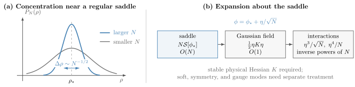
Increasing $N$ narrows the weight around a regular saddle by $N^{-1/2}$. With $\phi=\phi_\star+N^{-1/2}\eta$, the saddle action is $O(N)$, the Gaussian theory is $O(1)$, and fluctuation interactions carry explicit inverse powers of $N$.

Factorization and Observable Scaling

Let

$$\rho = \frac{1}{N} \sum_{a=1}^{N} O_a$$

be a normalized flavor-singlet collective observable. Away from singular points, a regular saddle commonly gives

$$\begin{aligned} \langle\rho\rangle &= \rho_\star + O\!\left(\frac{1}{N}\right), \\ \langle\rho^2\rangle_{\mathrm c} &= O\!\left(\frac{1}{N}\right). \end{aligned}$$

Consequently,

$$\langle\rho^2\rangle = \langle\rho\rangle^2 + O\!\left(\frac{1}{N}\right).$$

This is large-$N$ factorization for normalized singlets. It resembles a classical law of large numbers, but correlations among components are allowed and are often essential; the result follows from the effective-action scaling, not from assuming statistical independence.

For the unnormalized sum $R=N\rho$,

$$\langle R\rangle=O(N), \qquad \langle R^2\rangle_{\mathrm c}=O(N).$$

Its absolute fluctuation is therefore $O(\sqrt N)$ while its relative fluctuation is $O(N^{-1/2})$. Saying simply “fluctuations vanish” hides this normalization dependence.

Sources organize connected correlators

Introduce a source $J$ coupled to a normalized collective field:

$$Z_N[J] = \int\mathcal D\phi\, \exp\!\left\{ -N\mathcal S[\phi] + N\int_x J(x)\phi(x) \right\}.$$

Then

$$W_N[J] = \frac{1}{N} \ln Z_N[J]$$

has an $O(1)$ limit. Derivatives of $W_N$ generate normalized connected correlators with explicit powers of $1/N$. This source formulation is often the cleanest way to avoid guessing the scaling of a composite observable.

Worked Example: A Radial O(N) Integral

Consider the stable zero-dimensional vector integral

$$Z_N(r,u) = \int_{\mathbb R^N} d^N\boldsymbol\varphi\, \exp\!\left[ -\frac{r}{2} \boldsymbol\varphi^2 -\frac{u}{4N} \left(\boldsymbol\varphi^2\right)^2 \right], \qquad u>0.$$

It has no spatial dynamics, but it isolates three features that recur in many-body models:

• the quartic coupling must scale as $1/N$;
• the natural collective variable is $\boldsymbol\varphi^2/N$;
• the integration measure contributes an $O(N)$ entropic term.

Define

$$\rho = \frac{\boldsymbol\varphi^2}{N}, \qquad \rho\geq0.$$

Using

$$d^N\boldsymbol\varphi = \Omega_{N-1} R^{N-1}dR, \qquad \Omega_{N-1} = \frac{2\pi^{N/2}}{\Gamma(N/2)},$$

and $R=\sqrt{N\rho}$ gives

$$R^{N-1}dR = \frac{N^{N/2}}{2} \rho^{N/2-1}d\rho.$$

Therefore

$$Z_N = \mathcal C_N \int_0^\infty \frac{d\rho}{\rho} \exp\!\left[ -Nf(\rho) \right],$$

with

$$f(\rho) = \frac{r}{2}\rho + \frac{u}{4}\rho^2 -\frac{1}{2}\ln\rho.$$

The logarithm did not come from the Hamiltonian. It came from the surface area of the high-dimensional sphere. Dropping it would give the wrong leading saddle.

The stationary equation is

$$f'(\rho_\star) = \frac{r}{2} + \frac{u}{2}\rho_\star -\frac{1}{2\rho_\star} = 0,$$

or

$$u\rho_\star^2 + r\rho_\star -1 = 0.$$

The positive solution is

$$\rho_\star = \frac{ \sqrt{r^2+4u}-r }{2u}.$$

Moreover,

$$f''(\rho_\star) = \frac{u}{2} + \frac{1}{2\rho_\star^2} >0,$$

so the radial saddle is stable. To leading order,

$$\frac{1}{N} \left\langle \boldsymbol\varphi^2 \right\rangle = \rho_\star + O\!\left(\frac{1}{N}\right).$$

For $u\to0$ with $r>0$, $\rho_\star\to1/r$, exactly as expected for $N$ independent Gaussian components with variance $1/r$.

What this simple example teaches

The large-$N$ saddle balances energy and measure entropy. In an actual many-body system, the analogous entropy can come from:

• a determinant produced by integrating over $N$ matter fields;
• the multiplicity of microscopic states compatible with a collective field;
• momentum and frequency modes;
• a constraint or Jacobian associated with changing variables.

The leading effective action is therefore not obtained by minimizing the microscopic interaction energy alone.

Bosonic Example: The O(N) Vector Model

Consider $N$ real bosonic fields in Euclidean time:

$$\begin{aligned} S_E[\boldsymbol\varphi] &= \int_x \left[ \frac{1}{2} \sum_{a=1}^{N} \left( (\partial_\tau\varphi_a)^2 + c^2(\boldsymbol\nabla\varphi_a)^2 + r_0\varphi_a^2 \right) \right. \\ &\qquad\left. + \frac{u_0}{4N} \left( \sum_{a=1}^{N}\varphi_a^2 \right)^2 \right], \qquad u_0>0, \end{aligned}$$

where

$$\int_x \equiv \int_0^\beta d\tau \int d^d x.$$

The interaction is $O(N)$ when $\boldsymbol\varphi^2=O(N)$. This model can represent an $N$-component bosonic order parameter or the continuum limit of suitable quantum-rotor and spin systems. Its full critical theory requires renormalization; here it serves as a transparent large-$N$ construction.

Introducing one collective field

At each spacetime point, the Gaussian identity

$$\exp\!\left[ -\frac{u_0}{4N}X^2 \right] \propto \int_{-\infty}^{\infty} d\lambda\, \exp\!\left[ -\frac{N}{4u_0}\lambda^2 + \frac{i}{2}\lambda X \right]$$

applies for $u_0>0$. Here $X=\boldsymbol\varphi^2$. The auxiliary field $\lambda$ is real on the original contour, while its relevant saddle is generally reached after a contour deformation.

After the $N$ Gaussian matter fields are integrated out,

$$Z_N \propto \int\mathcal D\lambda\, e^{-S_{\mathrm{eff}}[\lambda]},$$

where

$$\begin{aligned} S_{\mathrm{eff}}[\lambda] &= N \left\{ \int_x \frac{\lambda^2}{4u_0} \right. \\ &\qquad\left. + \frac{1}{2} \operatorname{Tr}\ln \left[ -\partial_\tau^2 -c^2\nabla^2 + r_0 -i\lambda \right] \right\}. \end{aligned}$$

The factor of $N$ multiplying the trace logarithm comes from the $N$ identical components. This is the source of saddle control.

The Hubbard–Stratonovich identity is exact after its measure and contour are specified. Replacing the remaining $\lambda$ integral by one saddle is the approximation.

Uniform mass saddle

For a translation-invariant symmetric saddle, define

$$m^2 = r_0-i\lambda_\star.$$

Stationarity gives the regulated gap equation

$$m^2 = r_0 + u_0 T \sum_{\omega_n} \int_{\lvert\mathbf k\rvert<\Lambda} \frac{d^d k}{(2\pi)^d} \frac{1}{ \omega_n^2 + c^2\mathbf k^2 + m^2 }.$$

The ultraviolet cutoff $\Lambda$ is displayed because the integral is not automatically finite. A continuum prediction requires a regulator and a prescription relating $r_0,u_0$ to physical parameters.

The equation has a simple interpretation:

1. begin with a trial mass $m$;
2. compute the fluctuation variance of all bosonic components;
3. feed that variance back into the collective mass;
4. solve the resulting self-consistency condition.

At $N=\infty$, this resummation is the leading saddle rather than an arbitrary closure.

Broken-symmetry saddle

To allow a condensate or ordered component, write

$$\varphi_1(x) = \sqrt N\,\Phi + \pi_1(x),$$

with the other components unshifted. The uniform saddle equations have the schematic form

$$m^2\Phi=0,$$

and

$$m^2 = r_0 + u_0 \left[ \Phi^2 + T\sum_{\omega_n} \int^\Lambda \frac{d^d k}{(2\pi)^d} \frac{1}{ \omega_n^2+c^2\mathbf k^2+m^2 } \right].$$

Thus either $\Phi=0$ or the transverse mass vanishes at the leading ordered saddle. Dimension, temperature, finite volume, and infrared behavior decide whether this formal solution represents a legitimate phase.

The equation does not override theorems forbidding continuous-symmetry breaking in specified low-dimensional settings. It identifies a candidate saddle whose fluctuations must still be tested.

Fluctuations of the auxiliary field

Set

$$\lambda = \lambda_\star + \frac{1}{\sqrt N} \eta.$$

The quadratic kernel of $\eta$ contains a two-boson polarization function. Schematically,

$$K_\lambda(q) = \frac{1}{2u_0} + \frac{1}{2} \Pi(q;m),$$

where

$$\Pi(q;m) = T\sum_{\omega_n} \int_{\mathbf k} G_m(k)G_m(k+q).$$

The collective propagator is $K_\lambda^{-1}/N$ in the original normalization. Its poles and softening describe amplitude or constraint fluctuations. This is one place where large-$N$ Gaussian theory and RPA-like resummation meet, although their canonical formulations and channel conventions remain distinct.

A nonrelativistic cousin

An $N$-flavor Bose gas can be organized similarly:

$$\begin{aligned} S_E &= \int_x \left[ \sum_{a=1}^{N} \psi_a^\ast \left( \partial_\tau -\frac{\nabla^2}{2m} -\mu \right) \psi_a \right. \\ &\qquad\left. + \frac{g}{2N} \left( \sum_{a=1}^{N} \psi_a^\ast\psi_a \right)^2 \right]. \end{aligned}$$

A density-channel auxiliary field again produces an effective action proportional to $N$. The precise saddle and excitation content differ from the real-vector model because particle number, complex fields, and first-order imaginary-time dynamics matter. The shared lesson is the scaling $g/N$ and the concentration of a normalized flavor-singlet density.

Spin Example: An SU(N) Antiferromagnet

Large-$N$ spin methods replace the physical spin symmetry by a chosen family whose internal dimension can grow. A representative fermionic construction introduces partons

$$f_{i\alpha}, \qquad \alpha=1,\ldots,N,$$

with the local constraint

$$\sum_{\alpha=1}^{N} f_{i\alpha}^\dagger f_{i\alpha} = \kappa N,$$

where $0<\kappa<1$ is held fixed as $N\to\infty$. The $SU(N)$ generators can be represented as

$$S_i^{\alpha\beta} = f_{i\alpha}^\dagger f_{i\beta} -\kappa\delta^{\alpha\beta}.$$

The constraint selects a representation and removes unphysical number sectors. For $SU(2)$ spin $1/2$, one familiar fermionic representation has one parton per site, corresponding to $\kappa=1/2$. The continuation to general $N$ still requires a representation choice.

Exchange and bond scaling

Define the flavor-summed bond operator

$$B_{ij} = \sum_{\alpha=1}^{N} f_{i\alpha}^\dagger f_{j\alpha}.$$

Since $B_{ij}=O(N)$ at a flavor-symmetric saddle, a representative exchange channel has the scaling

$$H_J = -\frac{J}{N} \sum_{\langle ij\rangle} B_{ij}^\dagger B_{ij} + \text{constant}.$$

This form is one standard large-$N$ continuation of antiferromagnetic exchange. The additive constant and its relation to $S_i^{\alpha\beta}S_j^{\beta\alpha}$ depend on generator and constraint conventions.

A complex bond field $\chi_{ij}$ decouples the interaction:

$$\begin{aligned} H_{J,\mathrm{sp}} &= \sum_{\langle ij\rangle} \left[ \frac{N}{J} \lvert\chi_{ij}\rvert^2 \right. \\ &\qquad\left. -\chi_{ij}^\ast B_{ij} -\chi_{ij}B_{ij}^\dagger \right]. \end{aligned}$$

Stationarity yields

$$\chi_{ij} = \frac{J}{N} \langle B_{ij}\rangle.$$

The local constraint is imposed by a Lagrange-multiplier field $\lambda_i(\tau)$. Integrating the $N$ identical parton flavors produces

$$S_{\mathrm{eff}}[\chi,\lambda] = N\,s_{\mathrm{eff}}[\chi,\lambda].$$

The bond and constraint equations are therefore saddle equations at leading order in $1/N$.

Gauge redundancy is not optional

The parton representation is invariant under the local change

$$f_{i\alpha}(\tau) \longrightarrow e^{i\theta_i(\tau)} f_{i\alpha}(\tau).$$

Correspondingly,

$$\begin{aligned} \chi_{ij} &\longrightarrow e^{i[\theta_j-\theta_i]} \chi_{ij}, \\ \lambda_i &\longrightarrow \lambda_i-\partial_\tau\theta_i, \end{aligned}$$

for the convention in which the time derivative appears as $\partial_\tau+i\lambda_i$.

A nonzero $\chi_{ij}$ is therefore not by itself a gauge-invariant order parameter. Gauge-invariant information includes:

• the magnitude $\lvert\chi_{ij}\rvert$;
• symmetry-invariant bond patterns;
• products of bond phases around closed loops;
• physical spin correlations and response functions.

Zero modes generated by this redundancy must be gauge fixed or removed before evaluating a fluctuation determinant. Treating them as ordinary unstable modes gives nonsense.

What the spin saddle can reveal

Depending on the lattice, representation, and exchange channels, candidate saddles can describe:

• uniform or modulated bond amplitudes;
• valence-bond patterns;
• flux states defined by gauge-invariant loop phases;
• parton bands with gapless points or Fermi surfaces;
• magnetically ordered saddles in bosonic or mixed constructions;
• spin-liquid candidates whose finite-$N$ fate depends on gauge fluctuations and nonperturbative effects.

The leading large-$N$ saddle is a controlled result for the chosen $N\to\infty$ family. Calling the same state a phase of the physical $N=2$ model requires additional evidence.

Why different spin large-N limits differ

Fermionic $SU(N)$, bosonic $Sp(N)$, and other continuations can weight magnetic order, valence bonds, and gauge fluctuations differently. Even when two constructions reproduce the same local $SU(2)$ algebra at the physical point, their leading saddles need not agree.

A trustworthy use of the method therefore reports:

1. the enlarged symmetry group;
2. the parton statistics;
3. the local constraint and representation;
4. which ratios are held fixed as $N$ grows;
5. the exchange-channel scaling;
6. the gauge redundancy;
7. the evidence supporting continuation to the physical model.

Relation to Mean Field, RPA, and Variational States

Large-$N$ is an organizing principle, not one specific ansatz.

Method	Relationship to a large-N construction	Important distinction
mean field	often equals the leading stationary configuration	mean field can exist without a large parameter
Hartree or Hartree–Fock	may become leading in a flavor-scaled family	exchange and direct terms can have different N counting
Gross–Pitaevskii theory	a classical field can be a saddle	dilute-gas control and large-N control are different limits
BCS theory	pairing fields can be saddle variables	the physical flavor number may be small
RPA	often matches Gaussian collective fluctuations or a leading bubble hierarchy	not every approximation called RPA comes from one large-N family
variational state	a saddle state can define a trial wavefunction	fluctuation corrections need not preserve a variational upper bound
diagrammatic expansion	flavor sums assign powers of N to graphs	complete power counting depends on propagators, vertices, and representation

A saddle is more than a guessed factorization only when control is shown

The stationarity equation may be identical to a familiar mean-field equation. The extra content of a large-$N$ derivation is:

• an explicit family of microscopic models;
• an action with a leading factor of $N$;
• a defined fluctuation field with $N^{-1/2}$ normalization;
• a Hessian and correction hierarchy;
• criteria for when the hierarchy fails.

Without these ingredients, calling a mean field “the large-$N$ saddle” does not establish control.

Gaussian fluctuations and response

Suppose a source $J$ couples to a collective field $\phi$. Linearizing the saddle equation gives

$$\int_y K(x,y) \delta\phi(y) = \delta J(x).$$

Thus

$$\delta\phi = K^{-1}\delta J.$$

The same inverse Hessian governs Gaussian fluctuations and linear response. In many models, this inverse has the algebraic form of an RPA denominator. The connection is structural: both describe feedback around a stationary reference. Exact signs and kernels depend on the channel and source convention.

When the Expansion Is Controlled

A useful large-$N$ calculation should pass several tests.

The model sequence is explicit

The Hamiltonian or action must be defined for general $N$. The physical value and the quantities held fixed must be stated.

All leading terms have compatible scaling

Kinetic, interaction, constraint, and source terms intended to compete should have the same leading $N$ order. Otherwise the limit may be trivial or dominated by a term absent from the physical problem.

The saddle lies on a legitimate contour

For real positive Euclidean measures, this is often straightforward. For imaginary auxiliary couplings, chemical potentials, sign problems, or real-time contours, the saddle and contour deformation require justification.

The physical Hessian is regular

After constraints, symmetry collective coordinates, and gauge redundancy are handled, the relevant Hessian should have no unexplained negative or zero eigenvalues. A negative mode may signal an unstable saddle; a zero mode may signal symmetry, gauge redundancy, criticality, or a missed collective coordinate.

The target observable has known scaling

An $O(N)$ free energy, an $O(1)$ normalized density, and an exponentially small tunneling amplitude do not share one correction hierarchy. Normalize before assigning powers.

Infrared and ultraviolet behavior is controlled

Large $N$ does not remove ultraviolet divergences. It also does not prevent infrared enhancement from soft modes. A regulator, boundary conditions, and order of limits remain part of the answer.

Finite-N evidence is available

Useful checks include:

• exact solutions in special limits;
• symmetry and conservation laws;
• sum rules and positivity;
• numerical calculations at several finite $N$;
• comparison with experiment when the model is material specific;
• known weak-coupling, strong-coupling, or high-temperature expansions.

Failure Modes and Subtleties

Critical softening

If the smallest Hessian eigenvalue behaves as

$$\kappa_{\min} \longrightarrow 0,$$

then

$$\langle(\delta\phi)^2\rangle \sim \frac{1}{ N\kappa_{\min} }$$

can become large despite the factor $1/N$. A sufficiently narrow critical region can invalidate naive Gaussian power counting.

Large-$N$ methods can still compute nontrivial critical exponents, but doing so generally requires solving the critical theory and organizing singular diagrams rather than substituting the saddle into a regular expansion.

Goldstone and gauge zero modes

Continuous symmetry breaking produces flat directions related by the broken symmetry. Parton descriptions introduce gauge-equivalent directions. Their zero eigenvalues are not ordinary Gaussian oscillators.

Depending on the case, one must:

• introduce collective coordinates;
• divide by the symmetry-group volume;
• gauge fix and include the corresponding Jacobian;
• separate physical Goldstone modes from redundant gauge directions;
• keep finite volume until symmetry restoration is understood.

Competing saddles and first-order transitions

Iterative solvers can converge to metastable saddles. Local stability does not determine the global free energy. Near coexistence, exponentially small terms and interface contributions can matter for tunneling, nucleation, and finite-size rounding even though they are invisible in a power series in $1/N$.

Nonperturbative terms

An asymptotic expansion

$$\mathcal O_N \sim \sum_{k=0}^{\infty} \frac{a_k}{N^k}$$

cannot detect a contribution such as

$$\Delta\mathcal O_N \sim e^{-cN}, \qquad c>0.$$

Such terms can encode tunneling between saddles, instanton-like events, confinement effects, or level splittings. They are smaller than every power at large $N$ but can decide qualitative physics at finite $N$.

Noncommuting limits

The limits

$$N\to\infty, \qquad V\to\infty, \qquad \beta\to\infty, \qquad \Lambda\to\infty$$

perform different operations. For example:

• taking $N\to\infty$ first may freeze a collective field before finite-volume tunneling is considered;
• taking $V\to\infty$ first may select a broken-symmetry sector;
• taking $\beta\to\infty$ first may expose a level splitting that vanishes exponentially in $N$;
• removing a cutoff before renormalizing may make a formal gap equation meaningless.

The intended order should be written, not inferred.

Extrapolation to small N

A leading result at $N=\infty$ can be qualitatively useful at $N=2$, but there is no general error bound saying that it must be. Potential problems include:

• large coefficients multiplying $1/N$;
• an asymptotic rather than convergent series;
• topology or representation theory special to small $N$;
• gauge fluctuations that are weak at large $N$ but strong at physical $N$;
• a phase transition between $N=\infty$ and the target value;
• Berry phases or defects suppressed in the leading saddle.

The extrapolation is a physical inference, not a theorem.

Matrix and gauge-theory limits

For matrix-valued fields, the number of components can scale as $N^2$, and diagrams are often organized by topology while a combination such as a coupling times $N$ is held fixed. That counting is not the vector-model hierarchy derived above.

This preview does not develop planar diagrams, matrix integrals, gauge fixing in non-Abelian field theory, or double-scaling limits. Those are QFT topics, not a minor extension of the bosonic and spin examples here.

A Reliable Calculation Workflow

1. Define the family. Write the model for arbitrary $N$ and identify the physical target value.
2. Name the large object. State whether $N$ counts components, flavors, channels, representation size, or something else.
3. Choose normalized collective variables. Prefer variables that remain $O(1)$ as $N\to\infty$.
4. Scale every coupling. Check the $N$ order of kinetic, interaction, constraint, and source terms.
5. Fix the regulator and ensemble. State volume, boundary conditions, temperature, cutoff, and conserved quantities.
6. Derive the effective action. Track Jacobians, determinants, constants needed for free-energy comparisons, and auxiliary-field contours.
7. Find all relevant saddles. Use symmetry to classify them and compare their leading actions.
8. Audit the Hessian. Separate physical stable, unstable, symmetry, and gauge directions.
9. Compute observables consistently. Differentiate the same regulated generating functional or transform operators with the same approximation.
10. Estimate corrections. Include the Gaussian determinant or a known $1/N$ term when the claim needs it.
11. Check limits and identities. Test weak coupling, solvable limits, conservation laws, sum rules, and scaling.
12. Justify finite-N claims. Compare against independent analytical, numerical, or experimental evidence.

Common Mistakes

• Treating the number of particles, sites, or spatial volume as the same $N$ used in a component expansion.
• Adding components without rescaling the collective interaction.
• Calling any self-consistent equation a controlled saddle.
• Dropping a Jacobian or determinant that contributes at order $N$.
• Confusing an exact Hubbard–Stratonovich identity with an approximate saddle evaluation.
• Solving the stationary equation without comparing competing saddles.
• Evaluating a determinant before removing gauge or symmetry zero modes.
• Declaring all fluctuations small without specifying observable normalization.
• Ignoring ultraviolet regularization in a continuum gap equation.
• Ignoring critical or low-dimensional infrared enhancement.
• Assuming every approximation called RPA is the Gaussian sector of the same large-$N$ model.
• Treating a gauge-dependent parton bond field as a directly observable order parameter.
• Presenting a leading $N=\infty$ spin-liquid saddle as proof of a phase at $N=2$.
• Assuming the $1/N$ series converges.
• Forgetting exponentially small effects that can split finite-$N$ states or connect saddles.
• Mixing matrix-model counting with vector-model counting.

Exercises

1. Choose the coupling scaling. Let $X=\sum_{a=1}^{N}X_a$ with each $X_a=O(1)$. Suppose

   $$H_{\mathrm{int}} = \frac{g}{N^\alpha} X^2.$$

   Find the scaling of $H_{\mathrm{int}}$ with $N$. Which $\alpha$ makes it compete with an $O(N)$ one-body Hamiltonian?

Solution

Since $X=O(N)$,

$$X^2=O(N^2).$$

Therefore

$$H_{\mathrm{int}} = O\!\left(N^{2-\alpha}\right).$$

To compete with an $O(N)$ one-body term, require

$$2-\alpha=1,$$

so

$$\alpha=1.$$

This gives the standard collective scaling $gX^2/N$. The answer is conditional on $X_a=O(1)$ and coherent addition to $X=O(N)$; a different observable normalization or representation can require different counting.

2. Saddle width and free energy. For

   $$Z_N = \int_{-\infty}^{\infty} dx\, e^{-N(a/2)(x-x_0)^2}, \qquad a>0,$$

   compute $Z_N$, the variance of $x$, and the term proportional to $\ln N$ in $-\ln Z_N$.

Solution

The Gaussian integral is

$$Z_N = \sqrt{\frac{2\pi}{Na}}.$$

The normalized distribution has

$$\langle x\rangle=x_0, \qquad \langle(x-x_0)^2\rangle = \frac{1}{Na}.$$

Thus the width scales as $N^{-1/2}$. Finally,

$$-\ln Z_N = \frac{1}{2}\ln N + \frac{1}{2}\ln a -\frac{1}{2}\ln(2\pi).$$

The $\frac12\ln N$ term is the finite-dimensional analogue of a Gaussian fluctuation determinant.

3. Recover the radial saddle. Starting from

   $$Z_N = \int d^N\boldsymbol\varphi\, \exp\!\left[ -\frac r2\boldsymbol\varphi^2 -\frac{u}{4N} \left(\boldsymbol\varphi^2\right)^2 \right],$$

   derive the effective function $f(\rho)$ for $\rho=\boldsymbol\varphi^2/N$. Show that the noninteracting limit gives $\rho_\star=1/r$ for $r>0$.

Solution

With $R=\sqrt{N\rho}$,

$$d^N\boldsymbol\varphi \propto \rho^{N/2-1}d\rho.$$

The energetic exponential is

$$\exp\!\left[ -N \left( \frac r2\rho + \frac u4\rho^2 \right) \right].$$

Combining it with

$$\rho^{N/2-1} = \rho^{-1} \exp\!\left( \frac N2\ln\rho \right)$$

gives

$$f(\rho) = \frac r2\rho + \frac u4\rho^2 -\frac12\ln\rho.$$

Stationarity gives

$$u\rho_\star^2+r\rho_\star-1=0.$$

For $u=0$ and $r>0$,

$$\rho_\star=\frac1r.$$

Equivalently, expanding the positive root at small $u$ gives

$$\frac{\sqrt{r^2+4u}-r}{2u} = \frac1r + O(u).$$

The logarithmic measure term is essential for this result.

4. Derive the bosonic gap equation. From

   $$\frac{S_{\mathrm{eff}}[\lambda]}{N} = \int_x\frac{\lambda^2}{4u_0} + \frac12 \operatorname{Tr}\ln \left( -\partial_\tau^2-c^2\nabla^2+r_0-i\lambda \right),$$

   derive the uniform saddle equation and express it in terms of $m^2=r_0-i\lambda_\star$.

Solution

Use

$$\delta\operatorname{Tr}\ln A = \operatorname{Tr} \left( A^{-1}\delta A \right).$$

Here

$$\frac{\delta A}{\delta\lambda} = -i.$$

For a uniform saddle,

$$0 = \frac{\lambda_\star}{2u_0} -\frac i2 G_{\lambda_\star}(x,x).$$

Hence

$$-i\lambda_\star = u_0 G_{\lambda_\star}(x,x).$$

With $m^2=r_0-i\lambda_\star$ and a momentum cutoff,

$$G_{\lambda_\star}(x,x) = T\sum_{\omega_n} \int_{\lvert\mathbf k\rvert<\Lambda} \frac{d^d k}{(2\pi)^d} \frac{1}{ \omega_n^2+c^2\mathbf k^2+m^2 }.$$

Therefore

$$m^2 = r_0 + u_0 T\sum_{\omega_n} \int_{\lvert\mathbf k\rvert<\Lambda} \frac{d^d k}{(2\pi)^d} \frac{1}{ \omega_n^2+c^2\mathbf k^2+m^2 }.$$

The equation is regulator dependent until the bare parameters are matched or renormalized.

5. Count fluctuation vertices. Let

   $$Z_N = \int\mathcal D\phi\, e^{-N\mathcal S[\phi]}.$$

   Set $\phi=\phi_\star+\eta/\sqrt N$. Show that an $m$-leg vertex from the Taylor expansion of $\mathcal S$ scales as $N^{1-m/2}$. What are the cubic and quartic powers?

Solution

The $m$th term contains the overall factor $N$ and $m$ factors of $N^{-1/2}$:

$$N \left( \frac{\eta}{\sqrt N} \right)^m \sim N^{1-m/2}\eta^m.$$

Thus

$$V_3\eta^3 \sim N^{-1/2}, \qquad V_4\eta^4 \sim N^{-1}.$$

The quadratic term is $O(1)$, which is why the rescaled field $\eta$ has an $O(1)$ Gaussian propagator.

6. Normalized and unnormalized fluctuations. Suppose

   $$\rho = \frac1N\sum_a O_a$$

   has connected variance $C/N+O(N^{-2})$. Let $R=N\rho$. Find the leading connected variance and relative root-mean-square fluctuation of $R$ if $\langle\rho\rangle=\rho_\star+O(N^{-1})$ with $\rho_\star\neq0$.

Solution

Since $R=N\rho$,

$$\langle R^2\rangle_{\mathrm c} = N^2 \langle\rho^2\rangle_{\mathrm c} = CN + O(1).$$

The root-mean-square fluctuation is

$$\Delta R = \sqrt{CN} + O(N^{-1/2}),$$

while

$$\langle R\rangle = N\rho_\star + O(1).$$

Therefore

$$\frac{\Delta R}{\langle R\rangle} = \frac{\sqrt C}{\rho_\star} \frac1{\sqrt N} + O(N^{-3/2}).$$

Absolute fluctuations grow as $\sqrt N$, but relative fluctuations vanish as $N^{-1/2}$.

7. Gauge audit of a bond saddle. Under

   $$f_{i\alpha} \to e^{i\theta_i}f_{i\alpha},$$

   determine the transformation of

   $$B_{ij} = \sum_\alpha f_{i\alpha}^\dagger f_{j\alpha}$$

   and of $\chi_{ij}$ in the term $-\chi_{ij}^\ast B_{ij}+\text{h.c.}$. Is $\langle\chi_{ij}\rangle\neq0$ by itself a physical order parameter?

Solution

The bond operator transforms as

$$B_{ij} \longrightarrow e^{i(\theta_j-\theta_i)} B_{ij}.$$

For $\chi_{ij}^\ast B_{ij}$ to remain invariant,

$$\chi_{ij} \longrightarrow e^{i(\theta_j-\theta_i)} \chi_{ij}.$$

Thus $\chi_{ij}$ is gauge dependent. Its nonzero expectation in a gauge-fixed saddle is not by itself a physical order parameter. Gauge-invariant information includes $\lvert\chi_{ij}\rvert$, symmetry-invariant patterns, and loop products such as

$$\chi_{12}\chi_{23}\cdots\chi_{L1},$$

whose phase defines a gauge-invariant flux.

8. Beyond all orders. Two saddles have the same perturbative $1/N$ expansion for an observable, but tunneling produces a splitting $\Delta_N=Ae^{-cN}$ with $A,c>0$. Explain why no finite power series in $1/N$ detects the splitting. Estimate the value of $N$ beyond which $\Delta_N<\varepsilon$.

Solution

For every fixed integer $k>0$,

$$\lim_{N\to\infty} N^k e^{-cN} = 0.$$

Therefore $e^{-cN}$ is smaller than every power $N^{-k}$ at large $N$. All coefficients in its formal expansion in powers of $1/N$ vanish, so no finite perturbative order detects it.

The condition

$$Ae^{-cN}<\varepsilon$$

is equivalent to

$$N > \frac1c \ln\!\left( \frac A\varepsilon \right).$$

Although exponentially small at large $N$, the splitting can restore a unique finite-$N$ state or connect sectors that the leading saddle treats as disconnected.

Key Takeaways

• Large-$N$ control comes from an explicitly defined model family whose effective action scales with $N$.
• Component number, particle number, volume, occupancy, and matrix rank are different large parameters.
• Couplings must be scaled so that the desired kinetic, interaction, and constraint terms remain in competition.
• A regular saddle has fluctuations of order $N^{-1/2}$ in normalized collective fields.
• The leading saddle is $O(N)$, the Gaussian determinant is $O(1)$, and fluctuation interactions generate inverse powers of $N$.
• Measure factors and matter-field determinants can contribute at leading order and cannot be discarded.
• The $O(N)$ bosonic saddle produces a self-consistent mass equation; its continuum use still requires regulation and renormalization.
• $SU(N)$ spin saddles depend on the chosen representation and carry gauge redundancy; gauge-dependent parton fields are not direct observables.
• Critical softening, zero modes, competing saddles, noncommuting limits, and effects of order $e^{-cN}$ require separate treatment.
• Extrapolation from $N=\infty$ to a small physical $N$ is an inference that needs independent checks.

References

1. T. H. Berlin and M. Kac, “The Spherical Model of a Ferromagnet”, Physical Review 86, 821–835 (1952).
2. H. E. Stanley, “Spherical Model as the Limit of Infinite Spin Dimensionality”, Physical Review 176, 718–722 (1968).
3. J. Hubbard, “Calculation of Partition Functions”, Physical Review Letters 3, 77–78 (1959).
4. P. Coleman, “1/N Expansion for the Kondo Lattice”, Physical Review B 28, 5255–5262 (1983).
5. I. Affleck and J. B. Marston, “Large-n Limit of the Heisenberg–Hubbard Model: Implications for High-$T_c$ Superconductors”, Physical Review B 37, 3774–3777 (1988).
6. N. Read and S. Sachdev, “Large-N Expansion for Frustrated Quantum Antiferromagnets”, Physical Review Letters 66, 1773–1776 (1991).
7. M. Moshe and J. Zinn-Justin, “Quantum Field Theory in the Large N Limit: A Review”, Physics Reports 385, 69–228 (2003).
8. S. Sachdev, Quantum Phase Transitions, 2nd ed., Cambridge University Press (2011).
9. A. Auerbach, Interacting Electrons and Quantum Magnetism, Springer (1994).
10. P. Coleman, Introduction to Many-Body Physics, Cambridge University Press (2015).
11. A. Altland and B. Simons, Condensed Matter Field Theory, 2nd ed., Cambridge University Press (2010).
12. J. W. Negele and H. Orland, Quantum Many-Particle Systems, Westview Press (1998).
13. E. Fradkin, Field Theories of Condensed Matter Physics, 2nd ed., Cambridge University Press (2013).
14. J. Zinn-Justin, Quantum Field Theory and Critical Phenomena, 5th ed., Oxford University Press (2021).