Hubbard–Stratonovich Transformation Preview

The Hubbard–Stratonovich transformation replaces an exponential quadratic in some operator or bilinear by a Gaussian integral whose coupling to that quantity is linear. In a fermionic path integral, this converts a quartic matter interaction into a quadratic fermion action coupled to an ordinary commuting auxiliary field.

In its simplest normalized form,

$$\begin{aligned} e^{aX^2/2} &= \frac{1}{\sqrt{2\pi a}} \int_{-\infty}^{\infty} d\phi \\ &\quad\times \exp\left[ -\frac{\phi^2}{2a} +\phi X \right], \\ &\qquad a>0. \end{aligned}$$

The identity is exact. What happens next need not be. Integrating over every auxiliary-field configuration reproduces the original interaction; replacing the integral by one stationary configuration is a saddle-point or mean-field approximation; sampling it numerically introduces statistical and possibly time-discretization errors.

That separation is the main organizing principle:

$$\begin{gathered} \text{quartic interaction} \\ \downarrow \\ \text{exact identity} \\ \text{channel, normalized measure, contour} \\ \downarrow \\ \text{quadratic matter plus auxiliary field} \\ \downarrow \\ \text{integrate exactly or sample} \\ \text{or expand about saddles}. \end{gathered}$$

Canonical Scope

This page is the canonical home for:

• the normalized scalar, matrix, and functional Hubbard–Stratonovich identities;
• real versus imaginary couplings and the contour information hidden by schematic formulas;
• finite-regulator use with fermionic bilinears;
• density, magnetic, and pairing decoupling channels;
• the continuous and discrete decouplings of the shifted Hubbard interaction;
• integrating out quadratic fermions to obtain determinants, Pfaffians, and auxiliary-field effective actions;
• the precise point at which a mean field appears as a saddle;
• channel or Fierz ambiguity after truncation;
• the distinction among an auxiliary variable, an order parameter, and a propagating collective field;
• the determinant-quantum-Monte-Carlo bridge and its sign or phase problem;
• a reproducibility ledger for auxiliary-field calculations.

Neighboring pages retain separate ownership:

• Path Integrals for Many-Body Systems owns basis insertion, thermal closure, Trotter control, worldlines, and the wider exact-versus-approximate path-integral ledger.
• Mean-Field Theory owns generic factorization, restricted variation, self-consistency, thermodynamic comparison, and stability.
• Hartree–Fock Approximation owns the normal fermionic direct-and-exchange approximation.
• BCS Mean-Field Theory owns the superconducting gap equation, quasiparticle spectrum, and thermodynamics.
• Large-N and Saddle-Point Methods Preview owns control by component counting and systematic fluctuations about a saddle.
• Landau–Ginzburg Theory Preview owns static order-parameter functionals, symmetry-allowed terms, and critical coarse graining.
• Random Phase Approximation owns response-function resummation and collective poles.

The purpose here is to make the transformation itself auditable and to show exactly where those later descriptions begin.

Three Different Claims

An auxiliary-field derivation should keep three logical layers separate.

Representation. A normalized integral identity rewrites the same regulated partition function or amplitude. The channel, measure, constants, and contour are part of this claim.

Evaluation. The new integral is performed analytically, sampled numerically, expanded about one or more saddles, or truncated in some other way. Accuracy belongs to this layer.

Interpretation. The auxiliary field may be related to a density, magnetization, pair amplitude, or another composite operator. That relation depends on normalization, sources, symmetries, and the approximation used.

Calling the first layer exact does not certify the second or third. Conversely, a useful mean field does not make a carelessly normalized transformation an identity.

The Normalized Scalar Identity

Let $X$ be a commuting number, a single self-adjoint operator, or a Grassmann-even expression for which the formal power series is defined. For $a>0$,

$$\mathcal I_a[X] = \frac{1}{\sqrt{2\pi a}} \int_{\mathbb R} d\phi\, \exp\left[ -\frac{\phi^2}{2a} +\phi X \right].$$

Complete the square:

$$-\frac{\phi^2}{2a} +\phi X = -\frac{(\phi-aX)^2}{2a} +\frac{aX^2}{2}.$$

Translation invariance of the Gaussian measure then gives

$$\mathcal I_a[X] = e^{aX^2/2}.$$

For a bounded self-adjoint operator, the same statement follows by applying the scalar identity in its spectral representation. For an unbounded operator, domains and convergence have to be controlled. In a regulated fermionic coherent-state integral, $X$ is usually an even Grassmann polynomial, and equality can be checked term by term because the polynomial terminates.

Why the normalization matters

The factor $(2\pi a)^{-1/2}$ may cancel from a normalized expectation value when it is independent of all physical parameters. It does not automatically cancel from:

• a partition function or free energy;
• derivatives with respect to $a$;
• comparisons between channels with different measures;
• a discretized calculation in which one factor occurs at every site and time slice;
• a continuum limit where the determinant contributes a regulator-dependent constant.

Writing $\propto$ is acceptable during an intermediate derivation only if the discarded factor is restored before thermodynamic quantities are compared.

The opposite sign

For the same $a>0$,

$$\begin{aligned} e^{-aX^2/2} &= \frac{1}{\sqrt{2\pi a}} \int_{\mathbb R} d\phi \\ &\quad\times \exp\left[ -\frac{\phi^2}{2a} +i\phi X \right]. \end{aligned}$$

The Gaussian remains convergent on the real $\phi$ axis, but the linear coupling is imaginary. One can sometimes rotate the integration contour instead. That rotation is not a typographical change: orientation, normalization, convergence at infinity, singularities of the remaining integrand, and any $i0$ prescription must be retained.

The useful diagnostic is the sign in the Euclidean weight. If

$$S_{\mathrm{int}} = -\frac{a}{2}X^2,$$

then $e^{-S_{\mathrm{int}}}=e^{+aX^2/2}$ admits a real linear coupling. If $S_{\mathrm{int}}=+aX^2/2$, the real-axis formula uses $i\phi X$. Labels such as “repulsive” and “attractive” are not enough because algebraic channel identities can reverse the relevant sign.

Matrix and Functional Identities

Let $K$ be a real symmetric positive-definite $r\times r$ matrix and let the components of $J$ commute. Then

$$\begin{aligned} &\exp\left( \frac12 J^{\mathsf T}KJ \right) \\ &\quad= \frac{1}{ \sqrt{\det(2\pi K)} } \int_{\mathbb R^r} d^r\phi \\ &\quad\times \exp\Bigg[ -\frac12 \phi^{\mathsf T}K^{-1}\phi \\ &\qquad+ \phi^{\mathsf T}J \Bigg]. \end{aligned}$$

Diagonalizing $K$ reduces this formula to independent scalar Gaussians. This also reveals what changes outside the positive-definite case:

• a negative eigenvalue requires an imaginary coupling or a rotated contour;
• a zero eigenvalue cannot be inverted and must be separated as a constraint, gauge direction, or regulated mode;
• a complex kernel requires an integration cycle on which the Gaussian converges;
• noncommuting operator components do not inherit the matrix identity merely by replacing numbers with operators.

With a finite spacetime regulator, the same equation is an ordinary high-dimensional Gaussian identity. Functional notation abbreviates its continuum limit:

$$\begin{aligned} &\exp\left[ \frac12 \int_{x,y} J_a(x) K_{ab}(x,y) J_b(y) \right] \\ &\quad= \mathcal N_K \int\mathcal D\phi \\ &\quad\times \exp\Bigg[ -\frac12 \int_{x,y} \phi_a(x) K^{-1}_{ab}(x,y) \phi_b(y) \\ &\qquad+ \int_x \phi_a(x)J_a(x) \Bigg]. \end{aligned}$$

Here $\int_x$ may include space, imaginary time, lattice sites, internal indices, and time slices. The normalization is formally

$$\mathcal N_K = \bigl[\det(2\pi K)\bigr]^{-1/2},$$

but its meaning is inherited from the regulator. A continuum functional determinant is not a dimensionless number until the measure and ultraviolet prescription have been specified.

Local and nonlocal interactions

A local interaction has a kernel proportional to a spacetime delta function. Its auxiliary quadratic term is then local. For a nonlocal interaction $K(x,y)$, the auxiliary action contains $K^{-1}(x,y)$:

$$S_\phi = \frac12 \int_{x,y} \phi(x)K^{-1}(x,y)\phi(y).$$

“Localizing the fermion interaction” means making the matter action linear in the chosen bilinear. It does not guarantee that the auxiliary-field action is local. Coulomb, retarded, and projected interactions retain their kernel structure.

Fermionic Partial Bosonization

Consider a regulated Euclidean fermion action

$$S[\bar\psi,\psi] = S_0[\bar\psi,\psi] - \frac12 O_aK_{ab}O_b,$$

where each $O_a=\bar\psi\Gamma_a\psi$ is Grassmann even and repeated labels include all regulated coordinates. The weight contains

$$\exp\left( \frac12 O_aK_{ab}O_b \right).$$

The transformation gives

$$\begin{aligned} Z &= \mathcal N_K \int \mathcal D\phi\, \mathcal D\bar\psi\, \mathcal D\psi \\ &\quad\times \exp\left[ -S_0 -\frac12\phi_aK^{-1}_{ab}\phi_b +\phi_aO_a \right]. \end{aligned}$$

Equivalently, the auxiliary action is

$$S_{\mathrm{aux}} = S_0 + \frac12\phi_aK^{-1}_{ab}\phi_b - \phi_aO_a.$$

The matter fields now appear quadratically whenever $S_0$ is quadratic. The interaction has not disappeared; it is carried by exchange and fluctuations of $\phi$.

The auxiliary field is commuting even when the matter fields are fermionic. Its label reflects the chosen bilinear:

• a scalar density field couples to $\bar\psi\psi$ or a shifted density;
• a magnetic field couples to $\bar\psi\boldsymbol\sigma\psi$;
• a complex pairing field couples to two annihilation or two creation fields;
• bond, current, orbital, and multipolar fields arise from other channels.

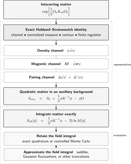
The channel, normalized measure, and contour belong to the exact identity. Integrating out quadratic matter gives an auxiliary-field effective action. Exact integration, Monte Carlo sampling, and saddle expansion are different ways of evaluating that new representation.

Density and Spin Channels in the Hubbard Model

For one spinful lattice orbital, define

$$\begin{aligned} n &= n_\uparrow+n_\downarrow, \\ m &= n_\uparrow-n_\downarrow, \\ q &= \left(n_\uparrow-\frac12\right) \left(n_\downarrow-\frac12\right). \end{aligned}$$

Using $n_\sigma^2=n_\sigma$, one obtains two exact operator identities:

$$q = \frac12(n-1)^2 - \frac14,$$

and

$$q = -\frac12m^2 + \frac14.$$

Thus the particle-hole-symmetric onsite interaction

$$H_U = Uq$$

can be written in a charge or an Ising-spin channel. The two representations are algebraically equal, including their constants.

Repulsive interaction in the spin channel

For $U>0$ and one imaginary-time step $\Delta\tau$,

$$\begin{aligned} e^{-\Delta\tau H_U} &= e^{-\Delta\tau U/4} \exp\left( \frac{\Delta\tau U}{2}m^2 \right) \\ &= \frac{e^{-\Delta\tau U/4}}{ \sqrt{2\pi\Delta\tau U} } \int_{\mathbb R} d\phi \\ &\quad\times \exp\left[ -\frac{\phi^2}{2\Delta\tau U} +\phi m \right]. \end{aligned}$$

The field is real and couples with opposite signs to up and down spin. In the charge representation,

$$\begin{aligned} e^{-\Delta\tau H_U} &= e^{+\Delta\tau U/4} \\ &\quad\times \exp\left[ -\frac{\Delta\tau U}{2}(n-1)^2 \right]. \end{aligned}$$

so a real integration variable on the original contour couples as $i\phi(n-1)$. A repulsive interaction therefore admits a real spin-channel decoupling and an imaginary-coupling charge decoupling. There is no contradiction: the exact algebra placed the same interaction on opposite sides of two squares.

The discrete Hirsch identity

The finite local Hilbert space also permits an exact sum over an Ising auxiliary variable $s=\pm1$:

$$\begin{aligned} &e^{-\Delta\tau U (n_\uparrow-\frac12) (n_\downarrow-\frac12)} \\ &\quad= \frac12 e^{-\Delta\tau U/4} \sum_{s=\pm1} e^{\lambda s (n_\uparrow-n_\downarrow)}, \end{aligned}$$

where

$$\cosh\lambda = e^{\Delta\tau U/2}.$$

Verification requires only the four local occupation states. Empty and doubly occupied states have $m=0$ and $q=1/4$; singly occupied states have $m=\pm1$ and $q=-1/4$. The right-hand side therefore produces respectively

$$\begin{gathered} e^{-\Delta\tau U/4}, \\ e^{-\Delta\tau U/4}\cosh\lambda = e^{+\Delta\tau U/4}. \end{gathered}$$

The identity is exact for the local interaction factor at every $\Delta\tau$. A finite-step factorization such as

$$e^{-\Delta\tau(K+H_U)} \approx e^{-\Delta\tau K} e^{-\Delta\tau H_U}$$

has a separate Trotter error. The exactness of the discrete decoupling does not remove that error.

An Atomic-Site Normalization Check

Set the hopping to zero and retain the shifted repulsive interaction $H_U=Uq$. The continuous spin-channel identity gives

$$\begin{aligned} Z_{\mathrm{at}} &= \operatorname{Tr} e^{-\beta Uq} \\ &= \frac{e^{-\beta U/4}}{ \sqrt{2\pi\beta U} } \int_{\mathbb R} d\phi\, e^{-\phi^2/(2\beta U)} \operatorname{Tr}e^{\phi m}. \end{aligned}$$

The trace over the four local states is

$$\operatorname{Tr}e^{\phi m} = 2+2\cosh\phi.$$

The Gaussian moments are

$$\begin{aligned} \frac{1}{\sqrt{2\pi\beta U}} \int d\phi\, e^{-\phi^2/(2\beta U)} &= 1, \\ \frac{1}{\sqrt{2\pi\beta U}} \int d\phi\, e^{-\phi^2/(2\beta U)} \cosh\phi &= e^{\beta U/2}. \end{aligned}$$

Therefore

$$Z_{\mathrm{at}} = 2e^{-\beta U/4} + 2e^{+\beta U/4},$$

which is exactly the spectral trace: two states have $q=1/4$ and two have $q=-1/4$. This small check catches a missing constant, an incorrect Gaussian width, or an omitted normalization immediately.

It also warns against interpreting the integration variable too quickly. There is no magnetic phase transition on one site. The integral sums all values of $\phi$, and its symmetry is not broken merely because $\phi$ couples to $m$.

Magnetic Auxiliary Fields

In a coherent-state action, a magnetic decoupling has the schematic form

$$\begin{aligned} S_{\mathrm{mag}} &= \int_x \left[ \frac{\mathbf M^2}{2g_m} - \mathbf M\cdot \mathbf m \right], \\ \mathbf m &= \bar\psi\, \boldsymbol\sigma \psi. \end{aligned}$$

Integrating over the three components of $\mathbf M$ generates the corresponding $\mathbf m^2$ interaction when the Grassmann-even components, normalization, and contour are treated consistently. A vector field makes spin-rotation covariance manifest. The discrete Ising decoupling instead chooses a spin axis for each auxiliary-field configuration; summing all configurations can restore the symmetry of the original partition function.

Several statements should not be collapsed:

• introducing $\mathbf M$ is an exact change of variables when the identity is exact;
• finding a stationary $\mathbf M_\star$ is an approximation unless a control limit makes the saddle exact;
• interpreting $\mathbf M_\star\neq0$ as magnetic order requires symmetry, source, volume, and stability analysis;
• interpreting fluctuations of $\mathbf M$ as magnons or paramagnons requires poles and residues of the matched response, not merely the field name.

The canonical definitions and thermodynamic-limit tests live on Order Parameters.

Operator and Grassmann identities are not interchangeable

At one time slice, different spin-operator components do not commute. A multicomponent Gaussian formula proved for commuting variables cannot be promoted blindly to $\exp(c\mathbf S^2)$ by placing $\mathbf S$ inside it. One must use:

• a verified finite-dimensional operator identity;
• an ordered product with its own discretization error; or
• a regulated coherent-state action where the relevant bilinears are Grassmann even and the quartic polynomial identity has been established.

This distinction is especially important when comparing rotationally invariant continuous fields with discrete axis-selecting transformations.

Pairing Fields

Let

$$B = \psi_\downarrow\psi_\uparrow, \qquad \bar B = \bar\psi_\uparrow\bar\psi_\downarrow.$$

For $g>0$, the normalized complex Gaussian identity is

$$\begin{aligned} e^{g\bar B B} &= \frac{1}{\pi g} \int_{\mathbb C} d(\operatorname{Re}\Delta)\, d(\operatorname{Im}\Delta) \\ &\quad\times \exp\left[ -\frac{|\Delta|^2}{g} +\Delta\bar B +\Delta^*B \right]. \end{aligned}$$

It follows by completing the square in the two real components of $\Delta$, or by expanding the nilpotent Grassmann-even sources. For an attractive onsite interaction

$$H_{\mathrm{int}} = -g\, n_\uparrow n_\downarrow = -g\,B^\dagger B,$$

the Euclidean weight contains precisely $e^{+\Delta\tau g\bar B B}$ on one time slice, with $g$ replaced by $\Delta\tau g$ in the identity.

The transformed action contains

$$S_\Delta = \int_x \left[ \frac{|\Delta|^2}{g} - \Delta\bar B - \Delta^*B \right].$$

At a stationary configuration,

$$\Delta_\star = g\langle B\rangle_{\Delta_\star}, \qquad \Delta_\star^* = g\langle\bar B\rangle_{\Delta_\star}.$$

These are the structural gap equations. Their spectrum, regularization, number equation, free-energy comparison, and physical solutions belong on BCS Mean-Field Theory.

Charge and phase

Under the global number symmetry

$$\psi \longmapsto e^{i\alpha}\psi,$$

the pair bilinear transforms as

$$B \longmapsto e^{2i\alpha}B.$$

The coupling remains invariant when

$$\Delta \longmapsto e^{2i\alpha}\Delta.$$

The auxiliary pairing field therefore carries the transformation law of a charge-two pair amplitude. That fact does not by itself prove spontaneous symmetry breaking. In a finite symmetry-preserving integral, $\langle\Delta\rangle$ vanishes unless a source or boundary prescription selects a phase, while invariant correlations may remain nonzero.

Determinant or Pfaffian?

Normal density and magnetic decouplings preserve a $\bar\psi M\psi$ quadratic form, whose Grassmann integral is a determinant. Pairing terms mix creation and annihilation variables. In a doubled Nambu notation one may write the result using a determinant with a compensating factor for doubling. In an undoubled antisymmetric Grassmann form,

$$S_{\mathrm F} = \frac12 \Psi^{\mathsf T} \mathcal A[\Delta] \Psi,$$

the integral is

$$\int\mathcal D\Psi\, e^{-\Psi^{\mathsf T}\mathcal A\Psi/2} = \operatorname{Pf}\mathcal A,$$

with

$$\bigl(\operatorname{Pf}\mathcal A\bigr)^2 = \det\mathcal A.$$

Replacing every Pfaffian by an unsigned square root of a determinant can lose a physically relevant sign or phase.

Integrating Out the Fermions

After a normal-channel decoupling, write

$$S_{\mathrm{aux}} = \frac12 \phi K^{-1}\phi + \bar\psi M[\phi] \psi,$$

where spacetime, mode, spin, and flavor indices are suppressed. The finite Grassmann Gaussian gives

$$\int \mathcal D\bar\psi\, \mathcal D\psi\, e^{-\bar\psi M[\phi]\psi} = \det M[\phi].$$

Hence

$$Z = \mathcal N_K \int\mathcal D\phi\, e^{-\phi K^{-1}\phi/2} \det M[\phi].$$

When a continuous logarithm and determinant branch have been fixed, this is often written as

$$Z = \mathcal N_K \int\mathcal D\phi\, e^{-S_{\mathrm{eff}}[\phi]},$$

with

$$S_{\mathrm{eff}}[\phi] = \frac12 \phi K^{-1}\phi - \operatorname{Tr}\ln M[\phi].$$

For $N_f$ identical fermion flavors, the trace-log is multiplied by $N_f$. That scaling is one route to a controlled large-$N$ saddle, provided the interaction and field are normalized consistently.

What the trace means

The trace in $\operatorname{Tr}\ln M$ runs over every index carried by the regulated fermion matrix:

• sites or momenta;
• imaginary-time slices or Matsubara frequencies;
• spin, orbital, band, and Nambu labels;
• any flavor multiplicity.

Its additive constants and branch are part of the definition. In infinite dimensions it generally needs regularization and, in a continuum theory, renormalization.

Hermiticity does not imply a positive weight

A Hermitian Hamiltonian ensures real physical energies and unitary real-time evolution. It does not ensure

$$\det M[\phi]\ge0$$

for every Euclidean auxiliary-field configuration. The determinant may be negative or complex because the decoupling, chemical potential, background field, or fermionic boundary conditions act on the one-body matrix in a way that does not preserve configuration-wise positivity.

Mean Field as a Saddle Point

Choose the coupling convention

$$S_{\mathrm{aux}} = \frac12\phi K^{-1}\phi - \phi_aO_a + S_0.$$

After integrating out matter, stationarity requires

$$\frac{\delta S_{\mathrm{eff}}}{ \delta\phi_a } = 0.$$

With the expectation value evaluated in the quadratic background $\phi_\star$, this becomes

$$\left(K^{-1}\phi_\star\right)_a = \langle O_a\rangle_{\phi_\star}.$$

Equivalently,

$$\phi_{\star,a} = K_{ab} \langle O_b\rangle_{\phi_\star}.$$

This is a self-consistency equation. It is the auxiliary-field version of a mean-field decoupling. The equation alone does not identify the physical solution: one must also compare stationary values of the appropriate thermodynamic potential, impose constraints, and test the fluctuation Hessian.

The exact identity and the saddle approximation occur on different lines:

$$\begin{aligned} e^{O K O/2} &= \mathcal N_K \int\mathcal D\phi \\ &\quad\times e^{-\phi K^{-1}\phi/2+\phi O}, \\[4pt] \int\mathcal D\phi\, e^{-S_{\mathrm{eff}}[\phi]} &\approx e^{-S_{\mathrm{eff}}[\phi_\star]} \\ &\quad\times \text{fluctuation factors}. \end{aligned}$$

The first equality may be exact even when the second approximation is poor.

Gaussian fluctuations

Write

$$\phi = \phi_\star+\eta.$$

The effective action expands as

$$\begin{aligned} S_{\mathrm{eff}}[\phi] &= S_{\mathrm{eff}}[\phi_\star] \\ &\quad+ \frac12 \eta_a \mathcal H_{ab} \eta_b + O(\eta^3), \end{aligned}$$

where

$$\mathcal H_{ab} = \left. \frac{\delta^2S_{\mathrm{eff}}}{ \delta\phi_a\delta\phi_b } \right|_{\phi_\star}.$$

For the convention above,

$$\mathcal H = K^{-1} - \chi_0[\phi_\star],$$

where $\chi_0$ is the connected susceptibility of the chosen bilinear in the quadratic saddle background, with all indices and signs defined by the source convention. Zeros of the analytically continued inverse fluctuation propagator can become collective modes.

A negative Hessian direction signals that the stationary point is unstable on the chosen integration cycle. A zero direction may arise from symmetry, gauge redundancy, a critical point, or an omitted constraint. Each case requires a different treatment.

Auxiliary Field Is Not Automatically an Order Parameter

The Gaussian identity itself gives exact relations between the auxiliary field and the decoupled operator. For the real-coupling matrix identity, conditional Gaussian averaging yields

$$\langle\phi_a\rangle = K_{ab} \langle O_b\rangle.$$

For connected two-point functions,

$$\begin{aligned} \langle\phi_a\phi_b\rangle_{\mathrm c} &= K_{ab} \\ &\quad+ K_{ac}K_{bd} \langle O_cO_d\rangle_{\mathrm c}. \end{aligned}$$

The first term is a contact contribution from the auxiliary Gaussian. For an imaginary coupling, the corresponding factors of $i$ change these relations. Thus even an exact auxiliary-field correlator is not numerically identical to the physical composite-operator correlator without matching.

Moreover, the rescaling

$$\phi \longmapsto c\phi$$

can be absorbed into the Gaussian kernel and Yukawa coupling. The partition function is unchanged after the Jacobian and normalization are handled, while the numerical value assigned to $\phi$ changes. A physical order parameter is defined through an operator, a source, and a symmetry transformation law, not through an arbitrary auxiliary normalization.

An auxiliary field can become a useful collective field when:

1. its source matching to a physical operator is explicit;
2. its low-energy two-point function develops the relevant pole or long-range correlation;
3. other fields have been integrated out in a controlled regime;
4. its normalization and operator mixing are tracked;
5. the effective action respects the required symmetries and Ward identities.

Channel Choice and Fierz Ambiguity

Fermionic anticommutation and completeness relations among spin or internal matrices allow one quartic interaction to be written in several bilinear channels. For the shifted one-site Hubbard operator, an explicit one-parameter family is

$$\begin{aligned} q &= \frac{\alpha}{2}(n-1)^2 - \frac{1-\alpha}{2}m^2 \\ &\quad+ \frac{1-2\alpha}{4}. \end{aligned}$$

Every value of $\alpha$ gives the same operator. At $\alpha=1$ it is the charge identity; at $\alpha=0$ it is the Ising-spin identity. If every resulting Gaussian field is integrated on the correct contour with the full normalization and constant, exact observables are independent of $\alpha$.

After a saddle, loop, local, or channel truncation, results can depend on $\alpha$. This is the Fierz ambiguity of a partially bosonized approximation. It is not an ambiguity of the original Hamiltonian. It diagnoses information discarded by the approximation.

How to use channel dependence

A careful calculation should:

• state the complete bilinear identity before decoupling;
• record constants and signs;
• identify which symmetries are manifest for each auxiliary configuration and which emerge only after integration;
• avoid introducing several fields that each reproduce the full interaction, which would double count it;
• vary an allowed channel parameter when feasible;
• treat strong channel dependence as an uncertainty signal;
• compare with symmetry constraints, weak- or strong-coupling limits, and independent methods.

Choosing a channel because it favors the desired ordered state is not evidence that the state is realized.

Determinant Quantum Monte Carlo Bridge

For a time-discretized lattice fermion model, a typical sequence is:

1. split $\beta$ into $M$ slices with $\Delta\tau=\beta/M$;
2. choose the order of kinetic and interaction factors;
3. apply an exact local auxiliary-field identity on every site and slice;
4. integrate the now-quadratic fermions;
5. sample the resulting field-dependent determinant weight.

For a discrete spin field $s_{i\ell}$, the result has the schematic form

$$\begin{aligned} Z_M &= \sum_{\{s_{i\ell}\}} W_{\mathrm B}[s]\, \det M_\uparrow[s]\, \det M_\downarrow[s] \\ &\quad+ O(\Delta\tau^p), \end{aligned}$$

where $p$ depends on the product formula. A common matrix structure is

$$M_\sigma[s] = I + B_{M,\sigma}[s_M] \cdots B_{1,\sigma}[s_1].$$

The bosonic factor $W_{\mathrm B}$ contains all discrete prefactors and any field-only action. The determinant compactly sums fermion permutations in the background $s$.

Exact, systematic, and statistical ingredients

The method combines several accuracy statements:

• the local Hirsch transformation is exact;
• the finite-$\Delta\tau$ kinetic–interaction product may have a systematic error;
• matrix products require numerical stabilization at large $\beta$;
• Monte Carlo averages have autocorrelation and sampling uncertainty;
• finite size and finite temperature require separate extrapolations;
• a sign or phase problem can produce exponentially poor signal-to-noise.

These errors should be reported separately rather than merged into one generic “Monte Carlo error.”

A standard sign-free case

For the repulsive one-band Hubbard model with real hopping on a bipartite lattice at particle-hole-symmetric half filling, the spin-channel transformation admits a particle-hole relation between the two spin determinants. In the standard formulation their product is nonnegative. This is a structural result for a specified Hamiltonian, boundary condition, and decoupling.

Generic doping, frustrating hopping, magnetic flux, spin imbalance, or other interactions can break the relation. An alternative exact decoupling may change the severity of the average sign without changing physical observables. The average sign is therefore a property of the representation and sampling measure, not an observable of the Hamiltonian.

The existence of special sign-free formulations does not contradict the computational hardness of the generic fermion sign problem.

The Sign Problem Preview owns the general cancellation and reweighting analysis, including determinant pairing, basis dependence, and the distinction between exact cures and constrained approximations.

Contours, Reality, and Convergence

A compact auxiliary-field formula should be read as an integration-cycle statement, not only an algebraic exponential.

Diagonalize the quadratic form

For a real symmetric kernel,

$$K = R^{\mathsf T} \operatorname{diag} (\kappa_1,\ldots,\kappa_r) R.$$

Each eigenmode can be inspected independently:

• $\kappa_j>0$ supports the ordinary real Gaussian for $e^{+\kappa_jJ_j^2/2}$;
• $\kappa_j<0$ supports a real Gaussian with imaginary linear coupling, or an explicitly rotated contour;
• $\kappa_j=0$ is not Gaussian-integrable through $K^{-1}$ and must be separated.

If a real field is retained while the wrong-sign quadratic term makes the weight grow at infinity, the functional integral is not defined merely because the formal completion of the square looks familiar.

Complex saddles

When the original contour produces a complex effective action, stationary points may lie off the real field space. Deforming toward steepest-descent cycles requires:

• analyticity in the region swept by the deformation;
• control of determinant zeros and logarithm branches;
• unchanged endpoints or asymptotic sectors;
• inclusion of every contributing cycle and its orientation;
• a prescription for Stokes transitions.

Selecting one visually convenient complex saddle is not equivalent to the original integral without this information.

From Auxiliary Fields to Effective Field Theory

Integrating out short-distance or gapped matter can produce an effective action for a slowly varying auxiliary field. A derivative expansion may take the form

$$\begin{aligned} S_{\mathrm{eff}}[\phi] &= \int_x \Bigg[ \frac{r}{2}\phi^2 + \frac{c}{2}(\nabla\phi)^2 \\ &\qquad+ \frac{d}{2}(\partial_\tau\phi)^2 + \frac{u}{4!}\phi^4 + \cdots \Bigg]. \end{aligned}$$

The displayed terms are schematic. Symmetry, dimensionality, conservation laws, gapless matter, and analytic continuation determine what is actually allowed. Complex or multicomponent fields can also carry symmetry-allowed first-order temporal terms. Integrating out a Fermi surface can generate nonlocal and nonanalytic kernels, so a local polynomial expansion is not automatic.

This is the bridge to statistical field theory and QFT:

• the auxiliary field supplies a bosonic variable coupled linearly to a composite operator;
• the fermion determinant generates its interactions and dynamics;
• a saddle gives a candidate mean-field phase;
• the Hessian gives a fluctuation propagator;
• coarse graining organizes relevant, marginal, and irrelevant couplings;
• source matching relates field correlators to measurable responses.

Landau–Ginzburg Theory Preview owns the static order-parameter functional, Statistical Field Theory Preview owns the regulated field measure and its fluctuation integral, while Why Many-Body Quantum Mechanics Leads to QFT places auxiliary fields among microscopic, collective, and quasiparticle fields.

A Reproducible Decoupling Ledger

Before trusting an auxiliary-field result, record the following.

Original regulated problem

• Hamiltonian or Euclidean action, including constants and chemical-potential shifts;
• spatial lattice, basis, ultraviolet cutoff, and time regulator;
• boundary and thermal conditions;
• ordering convention for fermion modes and Grassmann variables;
• exact interaction tensor and its symmetries.

Identity

• bilinear channel and any Fierz parameter;
• continuous, discrete, real, complex, or matrix auxiliary field;
• Gaussian width or discrete coupling;
• normalization and Jacobian;
• integration contour and convergence prescription;
• direct algebraic or finite-Hilbert-space verification.

Evaluation

• fields integrated exactly, sampled, or replaced by saddles;
• all saddle sectors and source limits;
• fluctuation order and expansion parameter;
• Trotter order and $\Delta\tau$ extrapolation;
• determinant or Pfaffian branch and stabilization method;
• sign or phase reweighting and average-sign diagnostics.

Validation

• free, atomic, and symmetry-protected limits;
• derivatives of the free energy against direct observables;
• Ward identities and sum rules;
• finite-size, finite-temperature, and regulator convergence;
• channel dependence after approximation;
• comparison with an independent representation or method.

Common Mistakes

• Calling the Hubbard–Stratonovich step a mean-field approximation. The integral identity can be exact; selecting a saddle is the approximation.
• Dropping normalization or constant shifts and then comparing free energies.
• Choosing a real field for a wrong-sign Gaussian without an imaginary coupling or contour prescription.
• Assuming “repulsive” always means an imaginary field; the sign depends on the algebraic channel in the Euclidean exponent.
• Treating noncommuting operator components as commuting entries of a matrix Gaussian identity.
• Equating an auxiliary field with a physical order parameter without source matching and normalization.
• Inferring spontaneous order from one finite-volume saddle while ignoring symmetry-related saddles.
• Decoupling the same interaction fully in several channels and thereby double counting it.
• Hiding Fierz-parameter dependence after a truncation.
• Replacing a Pfaffian by a positive square root of its determinant.
• Claiming that an exact discrete transformation removes finite-time-step error from a separate Trotter factorization.
• Assuming microscopic Hermiticity makes every configuration weight positive.
• Interpreting the average sign as a physical observable.
• Expanding a fermion determinant locally without checking for gapless, nonanalytic response.

Connections

• Sign Problem Preview owns average-sign collapse, sign-free mechanisms, and complexity limits.
• Hubbard Model supplies the canonical Hamiltonian, particle-hole convention, dimer, and strong-coupling physics.
• Mean-Field Theory develops the self-consistency and stability workflow used after choosing a saddle.
• Hartree–Fock Approximation treats normal density-matrix factorization.
• BCS Mean-Field Theory develops the pairing saddle and gap equation.
• Large-N and Saddle-Point Methods Preview explains when determinant scaling controls a saddle expansion.
• Susceptibilities defines the response functions entering the auxiliary-field Hessian.
• Random Phase Approximation develops the related Gaussian-response resummation.
• Thermal Green Functions fixes imaginary-time signs, boundary conditions, and Matsubara conventions.
• Order Parameters separates operators, sources, symmetry, and thermodynamic limits.
• Statistical Field Theory Preview distinguishes auxiliary variables from coarse order parameters and carries the exact field representation into sources, fluctuations, and coarse graining.

References

1. R. L. Stratonovich, “On a Method of Calculating Quantum Distribution Functions,” Soviet Physics Doklady 2, 416–419 (1958) – early Gaussian auxiliary-field representation.
2. J. Hubbard, “Calculation of Partition Functions”, Physical Review Letters 3, 77–78 (1959) – the transformation in quantum statistical mechanics.
3. R. Blankenbecler, D. J. Scalapino, and R. L. Sugar, “Monte Carlo Calculations of Coupled Boson–Fermion Systems. I”, Physical Review D 24, 2278–2286 (1981) – integrating out fermions and sampling the resulting bosonic effective action.
4. J. E. Hirsch, “Discrete Hubbard–Stratonovich Transformation for Fermion Lattice Models”, Physical Review B 28, 4059–4061 (1983), with erratum – the discrete Ising-field identity.
5. G. G. Batrouni and R. T. Scalettar, “Anomalous Decouplings and the Fermion Sign Problem”, Physical Review B 42, 2282–2289 (1990) – pairing-channel decoupling and representation dependence of the average sign.
6. M. Troyer and U.-J. Wiese, “Computational Complexity and Fundamental Limitations to Fermionic Quantum Monte Carlo Simulations”, Physical Review Letters 94, 170201 (2005) – generic complexity of the fermion sign problem.
7. F. F. Assaad and H. G. Evertz, “World-Line and Determinantal Quantum Monte Carlo Methods for Spins, Phonons and Electrons”, in Computational Many-Particle Physics, Lecture Notes in Physics 739, 277–356 (2008) – determinant algorithms, auxiliary fields, and stabilization.
8. T. Ayral, J. Vučičević, and O. Parcollet, “Fierz Convergence Criterion: A Controlled Approach to Strongly Interacting Systems with Small Embedded Clusters”, Physical Review Letters 119, 166401 (2017) – channel dependence as a truncation diagnostic.
9. S. Karakuzu, B. Cohen-Stead, C. D. Batista, S. Johnston, and K. Barros, “A Flexible Class of Exact Hubbard–Stratonovich Transformations”, Physical Review E 107, 055301 (2023) – exact continuous-to-discrete auxiliary-field families.
10. J. W. Negele and H. Orland, Quantum Many-Particle Systems, CRC Press (2018 reissue) – fermionic coherent-state integrals, auxiliary fields, and saddle expansions.
11. A. Altland and B. Simons, Condensed Matter Field Theory, 2nd ed., Cambridge University Press (2010) – partial bosonization, determinants, nonlinear field theories, and disorder decouplings.
12. P. Coleman, Introduction to Many-Body Physics, Cambridge University Press (2015) – auxiliary fields, mean-field theories, and large-component methods.

Exercises

1. Scalar Identity and Auxiliary Moments

Prove the normalized scalar identity by completing the square. Then compute the conditional mean and variance of $\phi$ at fixed $X$.

Solution

The exponent is

$$-\frac{\phi^2}{2a} +\phi X = -\frac{(\phi-aX)^2}{2a} +\frac{aX^2}{2}.$$

Shift to

$$\eta = \phi-aX.$$

The normalized integral over $\eta$ equals one, leaving $e^{aX^2/2}$. At fixed $X$, the distribution is Gaussian with center $aX$ and width squared $a$. Therefore

$$\mathbb E(\phi\mid X) = aX,$$

and

$$\operatorname{Var}(\phi\mid X) = a.$$

Averaging these conditional moments over the original degrees of freedom produces the one- and two-point matching relations quoted in the text.

2. Charge–Spin Identity

Using only $n_\sigma^2=n_\sigma$, verify both expressions for

$$q = \left(n_\uparrow-\frac12\right) \left(n_\downarrow-\frac12\right).$$

Then derive the one-parameter Fierz family.

Solution

Let $d=n_\uparrow n_\downarrow$. Then

$$q = d-\frac{n}{2}+\frac14.$$

Because

$$(n-1)^2 = n^2-2n+1 = 2d-n+1,$$

one finds

$$\frac12(n-1)^2-\frac14 = d-\frac n2+\frac14 = q.$$

Similarly,

$$m^2 = n_\uparrow+n_\downarrow-2d = n-2d,$$

so

$$-\frac12m^2+\frac14 = d-\frac n2+\frac14 = q.$$

Multiplying the charge identity by $\alpha$ and the spin identity by $1-\alpha$ gives

$$q = \frac{\alpha}{2}(n-1)^2 - \frac{1-\alpha}{2}m^2 + \frac{1-2\alpha}{4}.$$

3. Verify the Discrete Transformation

Check the Hirsch identity on all four occupation states and derive the condition on $\lambda$.

Solution

For $|0\rangle$ and $|\uparrow\downarrow\rangle$,

$$q = \frac14, \qquad m = 0.$$

The left-hand side is $e^{-\Delta\tau U/4}$, while the auxiliary sum is

$$\frac12e^{-\Delta\tau U/4} \sum_{s=\pm1}1 = e^{-\Delta\tau U/4}.$$

For $|\uparrow\rangle$ and $|\downarrow\rangle$,

$$q = -\frac14, \qquad m = \pm1.$$

The auxiliary sum becomes

$$e^{-\Delta\tau U/4} \cosh\lambda.$$

Equating this with $e^{+\Delta\tau U/4}$ gives

$$\cosh\lambda = e^{\Delta\tau U/2}.$$

Because the identity agrees on a complete occupation basis, it is an operator identity.

4. Atomic Partition Function

Evaluate the continuous spin-channel integral for the one-site shifted Hubbard interaction and compute $\langle q\rangle$ from the result.

Solution

The integral derived above gives

$$Z_{\mathrm{at}} = 4\cosh\left( \frac{\beta U}{4} \right).$$

Because

$$\langle q\rangle = -\frac{1}{\beta} \frac{\partial\ln Z_{\mathrm{at}}}{ \partial U },$$

we obtain

$$\langle q\rangle = -\frac14 \tanh\left( \frac{\beta U}{4} \right).$$

For repulsive $U$ at low temperature this tends to $-1/4$, corresponding to the two singly occupied states. At $U=0$, all four states are equally weighted and $\langle q\rangle=0$.

5. Pairing-Field Transformation Law

For the coupling

$$-\Delta\bar B-\Delta^*B,$$

derive the transformation of $\Delta$ under $\psi\mapsto e^{i\alpha}\psi$. Explain why a nonzero pairing saddle does not by itself prove finite-volume symmetry breaking.

Solution

The pair operators transform as

$$B \longmapsto e^{2i\alpha}B, \qquad \bar B \longmapsto e^{-2i\alpha}\bar B.$$

Both couplings are invariant if

$$\Delta \longmapsto e^{2i\alpha}\Delta, \qquad \Delta^* \longmapsto e^{-2i\alpha}\Delta^*.$$

Thus $\Delta$ has the same number charge as $B$. In a finite system with no symmetry-breaking source, integrating over the global phase sums all symmetry-related configurations and gives $\langle\Delta\rangle=0$. A chosen saddle fixes one phase and is a symmetry-breaking approximation or a source-selected sector. Physical order requires the appropriate source and thermodynamic limits or an invariant long-range-correlation criterion.

6. Saddle Equation and Hessian

Starting from

$$S_{\mathrm{eff}}[\phi] = \frac12\phi K^{-1}\phi - \operatorname{Tr}\ln M[\phi],$$

with

$$M[\phi] = M_0-\phi_a\Gamma_a,$$

derive the saddle equation and state the meaning of the Hessian.

Solution

Using

$$\delta\operatorname{Tr}\ln M = \operatorname{Tr} \left( M^{-1}\delta M \right),$$

one obtains

$$\frac{\delta S_{\mathrm{eff}}}{ \delta\phi_a } = \left(K^{-1}\phi\right)_a + \operatorname{Tr} \left( G[\phi]\Gamma_a \right).$$

For the Euclidean Grassmann convention,

$$\langle O_a\rangle_\phi = -\operatorname{Tr} \left( G[\phi]\Gamma_a \right).$$

Stationarity therefore gives

$$\left(K^{-1}\phi_\star\right)_a = \langle O_a\rangle_{\phi_\star}.$$

Differentiating again gives the inverse propagator for Gaussian auxiliary-field fluctuations. With the source conventions of the text it is $K^{-1}-\chi_0$. Positive directions are locally stable on a real contour, zero directions require special treatment, and negative directions show that the saddle is not a local minimum on that contour.

7. Exact Equivalence versus Channel-Dependent Saddles

Two calculations use different values of $\alpha$ in the one-parameter Hubbard identity. Both retain every auxiliary-field configuration and use correct contours. A third calculation keeps only a uniform static saddle. Which results must agree, and what does disagreement diagnose?

Solution

The first two calculations are exact representations of the same regulated operator. Their partition functions and physical observables must agree after normalizations, constants, and regulator limits are handled consistently. Disagreement between them signals an implementation error or an invalid contour manipulation.

The uniform-static saddle discards spatial, temporal, and non-Gaussian fluctuations. Its result can depend on $\alpha$ because different exact representations distribute those discarded effects differently between the saddle and fluctuations. That dependence diagnoses truncation uncertainty; it is not a physical dependence of the Hubbard model.

8. An Indefinite Kernel

Let

$$\begin{gathered} K = \begin{pmatrix} k_+ & 0 \\ 0 & -k_- \end{pmatrix}, \\ k_+>0, \quad k_->0. \end{gathered}$$

Give a convergent real-axis auxiliary representation of $\exp(J^{\mathsf T}KJ/2)$ and explain what would fail if both linear couplings were chosen real.

Solution

The exponential factors as

$$\exp\left( \frac{k_+J_+^2}{2} \right) \exp\left( -\frac{k_-J_-^2}{2} \right).$$

A convergent representation is

$$\begin{aligned} &\frac{1}{ 2\pi\sqrt{k_+k_-} } \int_{\mathbb R^2} d\phi_+\,d\phi_- \\ &\quad\times \exp\Bigg[ -\frac{\phi_+^2}{2k_+} -\frac{\phi_-^2}{2k_-} \\ &\qquad+ \phi_+J_+ +i\phi_-J_- \Bigg]. \end{aligned}$$

The negative eigenmode requires the imaginary coupling. If both couplings were real while the Gaussian widths remained positive, integrating the second field would generate $e^{+k_-J_-^2/2}$, the wrong sign. Changing the quadratic term instead would make the real-axis Gaussian divergent. A contour rotation can provide an equivalent formulation only when its Jacobian, orientation, and convergence sectors are included.