Nonrelativistic Field Theory from Many-Body QM

A nonrelativistic field theory describes particles by operators such as $\psi_a(\mathbf x,t)$ that create and remove local excitations. For a specified one-particle space, regulator, and many-body Hamiltonian, this can be an exact rewriting of ordinary many-particle quantum mechanics. When a finite-range interaction is replaced by contact operators and a derivative expansion, the same language becomes an effective field theory whose couplings must be matched to measured or microscopic scattering data.

Continue on QFT.org selects the next field-theory route once the observable, regulator, state, and required continuum limit are fixed.

The characteristic local structure is

$$\begin{aligned} H &= \int d^d x\, \mathcal H, \\ S &= \int dt\,d^d x\, \left[ i\hbar\psi^\dagger\partial_t\psi - \mathcal H \right]. \end{aligned}$$

The first-order time derivative, the equal-time field algebra, and the absence of an independent antiparticle branch distinguish a Schrödinger field from a relativistic scalar field. The resulting theory is nevertheless a genuine quantum field theory: it has local operator fields, infinitely many continuum modes, correlation functions, ultraviolet regularization, renormalized couplings, and symmetry identities.

Canonical Scope

This page owns the technical bridge from a number-conserving many-body Hamiltonian to nonrelativistic field theory. It develops:

• the relation between first-quantized, Fock-space, and local-field descriptions;
• Hamiltonian densities and Lorentzian Schrödinger-field actions;
• the global $U(1)$ symmetry, number density, current, and Galilean structure;
• free propagators and the meaning of interaction vertices;
• contact interactions as regulated low-energy operators;
• matching to scattering length and effective range;
• $z=2$ power counting and its limits;
• continuum limits of lattice models;
• representative Bose- and Fermi-gas applications;
• the boundary between an exact rewriting, an EFT truncation, a saddle-point approximation, and a nonrelativistic limit of relativistic QFT.

Several neighboring pages retain their canonical material:

• Field Operators in Many-Body Models owns the field algebra, mode expansions, and explicit conversion of model Hamiltonians.
• Many-Particle Hamiltonians owns the systematic first- to second-quantized operator derivation.
• Green Functions in Many-Body QM owns Lehmann representations, statistics-dependent orderings, and spectral sum rules.
• Coherent-State Path Integrals Preview owns the finite-slice derivation, normal symbols, Grassmann variables, and thermal boundary conditions.
• Why Many-Body QM Leads to QFT owns the conceptual route map.

Conventions and Three Levels of Description

Unless stated otherwise, $\psi$ is a single-species bosonic operator field in $d$ spatial dimensions. The potential $V(\mathbf x,t)$ is real, and the interaction is local and number conserving. Internal indices will be displayed when they matter.

It is essential to distinguish three objects often denoted by the same letter:

Object	Meaning	Algebra
$\widehat\psi(\mathbf x,t)$	Heisenberg or Schrödinger operator-valued distribution	commutes or anticommutes at equal time
$\psi(\mathbf x,t)$ in a bosonic functional integral	ordinary complex integration variable	commuting number
$\psi(\mathbf x,t)$ in a fermionic functional integral	Grassmann integration variable	anticommuting generator

An operator identity is not automatically a pointwise identity for a functional-integral variable. Conversely, a saddle-point field is not automatically the exact expectation value of the operator field.

There are also three logical levels:

1. Exact regulated rewriting. A finite mode basis or spatial lattice gives a Fock-space theory exactly equivalent to the original many-particle Hamiltonian in each number sector.
2. Continuum effective theory. Short-distance dynamics is represented by local operators with cutoff-dependent coefficients matched to low-energy data.
3. Approximate solution. Perturbation theory, a saddle point, a loop expansion, or a numerical truncation is used to calculate observables.

Calling all three steps “second quantization” hides where assumptions enter.

Local Fields Are Operator-Valued Distributions

For bosons,

$$\begin{aligned} [\psi_a(\mathbf x),\psi_b^\dagger(\mathbf y)] &= \delta_{ab}\, \delta^{(d)}(\mathbf x-\mathbf y), \\ [\psi_a(\mathbf x),\psi_b(\mathbf y)] &= 0. \end{aligned}$$

For fermions, the corresponding anticommutators are

$$\begin{aligned} \{\psi_a(\mathbf x),\psi_b^\dagger(\mathbf y)\} &= \delta_{ab}\, \delta^{(d)}(\mathbf x-\mathbf y), \\ \{\psi_a(\mathbf x),\psi_b(\mathbf y)\} &= 0. \end{aligned}$$

The delta distribution means that $\psi(\mathbf x)$ is not generally an ordinary operator at an exact point. A mathematically safer object is the smeared field

$$\psi[f] = \int d^d x\, f^*(\mathbf x)\psi(\mathbf x),$$

for a suitable one-particle wavefunction $f$. Products at coincident points require a regulator and, in a continuum theory, may require composite-operator renormalization. Symbols such as $\delta^{(d)}(\mathbf0)$ are therefore warnings about an unresolved ultraviolet limit, not large physical numbers.

With a complete orthonormal basis $\{\varphi_\alpha\}$,

$$\psi(\mathbf x) = \sum_\alpha \varphi_\alpha(\mathbf x)a_\alpha.$$

The field has spatial dimension

$$[\psi] = L^{-d/2},$$

so that

$$N = \int d^d x\, \psi^\dagger\psi$$

is dimensionless. The continuum field packages all one-particle modes; it is not a wavefunction normalized to one particle.

Exact Conversion of a Many-Particle Hamiltonian

Consider identical particles with

$$\begin{aligned} H_N &= \sum_{i=1}^{N} \left[ -\frac{\hbar^2\nabla_i^2}{2m} + V(\mathbf x_i) \right] \\ &\quad+ \frac12 \sum_{i\ne j} U(\mathbf x_i-\mathbf x_j). \end{aligned}$$

The corresponding Fock-space operator is

$$\begin{aligned} H &= H_0 + H_{\mathrm{int}}, \\ H_0 &= \int d^d x\, \psi^\dagger(\mathbf x) h_0 \psi(\mathbf x), \\ h_0 &= -\frac{\hbar^2\nabla^2}{2m} + V(\mathbf x), \\ H_{\mathrm{int}} &= \frac12 \int d^d x\,d^d y\, \psi^\dagger(\mathbf x) \psi^\dagger(\mathbf y) \\ &\quad\times U(\mathbf x-\mathbf y) \psi(\mathbf y) \psi(\mathbf x). \end{aligned}$$

Restricting this operator to the $N$-particle sector reproduces $H_N$ with the appropriate exchange symmetry. This statement is exact when:

• the one-particle Hilbert space and boundary conditions agree;
• the same regulator is used on both sides;
• the field algebra matches the particle statistics;
• domains of unbounded operators are controlled;
• interaction kernels and operator ordering are identical.

The change of language does not itself add particle creation, relativity, or vacuum polarization. A number-conserving field Hamiltonian can be block diagonal in every fixed-$N$ sector.

Hamiltonian Density

For a short-range interaction at leading order in a low-momentum expansion, a common bosonic Hamiltonian density is

$$\begin{aligned} \mathcal H &= \frac{\hbar^2}{2m} \nabla\psi^\dagger \mathbin{\cdot} \nabla\psi \\ &\quad+ V(\mathbf x,t) \psi^\dagger\psi + \frac{g_0}{2} \psi^\dagger\psi^\dagger\psi\psi. \end{aligned}$$

Here $g_0$ is a bare coupling associated with a declared spatial regulator. The subscript is not cosmetic: in dimensions where the contact theory is ultraviolet divergent, $g_0$ must vary with the cutoff so that physical scattering data remain fixed.

In a grand-canonical description, introduce

$$K = H-\mu N.$$

Its density is obtained by replacing $V$ with $V-\mu$. The thermal ensemble uses $K$ in $e^{-\beta K}$. In real time one must state whether operators evolve with $H$ or with $K$; the two conventions differ by a number-dependent phase when $[H,N]=0$.

For two fermion components, a local $s$-wave interaction instead has the form

$$\mathcal H_{\mathrm{int}} = g_0\, \psi_\uparrow^\dagger \psi_\downarrow^\dagger \psi_\downarrow \psi_\uparrow.$$

A same-component zero-range $s$-wave monomial vanishes for fermions after proper regularization because of antisymmetry. Identical fermions first interact through higher-partial-wave or derivative operators unless additional internal structure is present.

Lorentzian Schrödinger-Field Action

The operator equations can be encoded by the formal Lorentzian action

$$\begin{aligned} S &= \int dt\,d^d x\, \mathcal L, \\ \mathcal L &= i\hbar \psi^\dagger\partial_t\psi - \mathcal H. \end{aligned}$$

For the contact model,

$$\begin{aligned} \mathcal L &= i\hbar \psi^\dagger\partial_t\psi - \frac{\hbar^2}{2m} \nabla\psi^\dagger \mathbin{\cdot} \nabla\psi \\ &\quad- (V-\mu) \psi^\dagger\psi - \frac{g_0}{2} \psi^\dagger\psi^\dagger\psi\psi. \end{aligned}$$

The symmetrized kinetic term

$$\frac{i\hbar}{2} \left( \psi^\dagger\partial_t\psi - (\partial_t\psi^\dagger)\psi \right)$$

differs from $i\hbar\psi^\dagger\partial_t\psi$ by a total time derivative. That boundary term can matter for open kernels and variational endpoint data, even though it does not alter bulk equations under compatible boundary conditions.

Varying $\psi^\dagger$ gives

$$i\hbar\partial_t\psi = \left[ -\frac{\hbar^2\nabla^2}{2m} + V-\mu + g_0\psi^\dagger\psi \right]\psi.$$

At the operator level, this is the Heisenberg equation with the displayed normal ordering. In a bosonic path integral it is the stationary-field equation. Replacing the operator by a complex field and then solving this equation is a mean-field step, not an exact consequence for every state.

Why the Time Derivative Is First Order

The Schrödinger-field action is first order in time because $\psi$ and $i\hbar\psi^\dagger$ form a canonical pair. Formally,

$$\pi_\psi = \frac{\partial\mathcal L} {\partial(\partial_t\psi)} = i\hbar\psi^\dagger.$$

The conjugate momentum of $\psi^\dagger$ vanishes in the unsymmetrized convention, so a classical constrained-Hamiltonian analysis contains second-class constraints. Quantization recovers the equal-time commutator or anticommutator rather than two independent oscillator coordinates at every point.

This structure has three consequences:

• initial data specify one complex field rather than an independent field and time derivative;
• the free inverse propagator is linear in frequency;
• a number-conserving vacuum theory has a particle branch without a separate negative-frequency antiparticle branch.

None of these statements says that the Hamiltonian is first order in spatial gradients. For ordinary massive particles, the leading kinetic operator is $-\hbar^2\nabla^2/(2m)$.

Global U(1) Symmetry and Number Conservation

The number-conserving action is invariant under

$$\begin{aligned} \psi &\longmapsto e^{i\alpha}\psi, \\ \psi^\dagger &\longmapsto e^{-i\alpha}\psi^\dagger, \end{aligned}$$

for constant $\alpha$. The corresponding density and current are

$$\begin{aligned} n(\mathbf x,t) &= \psi^\dagger\psi, \\ \mathbf j_N(\mathbf x,t) &= \frac{\hbar}{2mi} \left[ \psi^\dagger\nabla\psi - (\nabla\psi^\dagger)\psi \right]. \end{aligned}$$

Using the field equation and its adjoint gives the local continuity equation

$$\partial_t n + \nabla\mathbin{\cdot}\mathbf j_N = 0.$$

If the boundary flux vanishes,

$$\frac{dN}{dt} = 0, \qquad N = \int d^d x\,n.$$

The local statement is stronger than the integrated one because it also identifies how number is transported. Coupling the theory to external scalar and vector sources promotes the bookkeeping phase to a local transformation and generates current Ward identities. The full symmetry-to-current logic is developed in From Quantum Generators to Noether Currents.

Number conservation does not require the state to have a sharp particle number. A coherent superposition of number sectors can evolve under a number-conserving Hamiltonian, although superselection or preparation constraints may limit which relative phases are observable.

A term such as

$$\Delta^*\psi\psi + \Delta\psi^\dagger\psi^\dagger$$

is not invariant under the particle-number $U(1)$ unless $\Delta$ transforms as a charge-two field. In a mean-field pairing Hamiltonian this term can break number conservation at the auxiliary level even when the underlying microscopic theory conserves total number.

Galilean Structure and the Mass Charge

In free space, with interactions depending only on relative coordinates, the theory can be invariant under Galilean boosts. An active boost by velocity $\mathbf v$ acts on a field of mass $m$ as

$$\begin{aligned} \psi_{\mathbf v}(\mathbf x,t) &= \exp \left[ \frac{im}{\hbar} \left( \mathbf v\mathbin{\cdot}\mathbf x - \frac{\mathbf v^2t}{2} \right) \right] \\ &\quad\times \psi(\mathbf x-\mathbf vt,t). \end{aligned}$$

The phase is required by the Schrödinger kinetic term. It implies

$$\begin{aligned} n_{\mathbf v}(\mathbf x,t) &= n(\mathbf x-\mathbf vt,t), \\ \mathbf j_{N,\mathbf v}(\mathbf x,t) &= \mathbf j_N(\mathbf x-\mathbf vt,t) \\ &\quad+ \mathbf v\, n(\mathbf x-\mathbf vt,t). \end{aligned}$$

The momentum and boost generators can be written

$$\begin{aligned} \mathbf P &= \int d^d x\, \psi^\dagger(-i\hbar\nabla)\psi, \\ \mathbf K(t) &= m\int d^d x\, \mathbf x\,n - t\mathbf P. \end{aligned}$$

Their algebra contains

$$[K_i,P_j] = i\hbar\delta_{ij}\,mN.$$

Thus total mass is the central charge of the Galilei algebra. A trap, an external medium, spin–orbit coupling, or a spatial lattice generally breaks boost symmetry. Particle-number conservation can survive even when Galilean invariance does not.

Free Modes and the Propagator

For a translation-invariant grand-canonical generator,

$$K_0 = \int\frac{d^d k}{(2\pi)^d}\, \xi_{\mathbf k} a_{\mathbf k}^\dagger a_{\mathbf k},$$

where

$$\xi_{\mathbf k} = \frac{\hbar^2\mathbf k^2}{2m} - \mu.$$

Define the free retarded propagator by

$$G_0^R(t,\mathbf k) = -\frac{i}{\hbar} \Theta(t) \left\langle [a_{\mathbf k}(t),a_{\mathbf k}^\dagger(0)]_\eta \right\rangle,$$

where $[A,B]_\eta$ is a commutator for bosons and an anticommutator for fermions. Fourier transformation gives

$$G_0^R(\omega,\mathbf k) = \frac{1} {\hbar\omega-\xi_{\mathbf k}+i0}.$$

For $\mu=0$, its position-space form is

$$\begin{aligned} G_0^R(t,\mathbf x) &= -\frac{i}{\hbar} \Theta(t) \left( \frac{m}{2\pi i\hbar t} \right)^{d/2} \\ &\quad\times \exp \left( \frac{im\mathbf x^2}{2\hbar t} \right). \end{aligned}$$

It is the retarded inverse of the Schrödinger operator:

$$\left( i\hbar\partial_t + \frac{\hbar^2\nabla^2}{2m} \right) G_0^R(t,\mathbf x) = \delta(t)\delta^{(d)}(\mathbf x).$$

The $i0$ prescription is not determined by the classical differential operator alone. It records the boundary condition and ordering. Time-ordered, advanced, Matsubara, lesser, and greater propagators encode different physical questions and states.

In momentum space, the quadratic Lorentzian action is schematically

$$S_0 = \int_{\omega,\mathbf k} \psi^\dagger(\omega,\mathbf k) \left( \hbar\omega-\xi_{\mathbf k} \right) \psi(\omega,\mathbf k).$$

The propagator is the inverse quadratic kernel after a contour prescription is supplied. A quartic contact term is a local four-leg vertex that conserves energy, momentum, and particle number. Diagrammatic rules are therefore a compact expansion of the same many-body evolution, not pictures of literal particle trajectories.

Contact Interactions Are Effective Operators

A microscopic potential with range $R$ can be replaced at momenta $kR\ll1$ by a derivative expansion,

$$\begin{aligned} \mathcal L_{\mathrm{int}} &= -\frac{C_0}{2} (\psi^\dagger\psi)^2 \\ &\quad- \frac{C_2}{2} \left[ \nabla(\psi^\dagger\psi) \right]^2 + \cdots. \end{aligned}$$

The ellipsis contains every operator allowed by the declared symmetries, ordered by low-energy importance. The coefficient $C_0$ reproduces leading $s$-wave scattering; derivative terms encode effective range and shape parameters. Spin, statistics, external fields, and broken symmetries change the operator basis.

A contact term is therefore not a claim that the microscopic force is a fundamental delta function at arbitrarily short distance. It is a compact description of unresolved physics below a cutoff.

Three-Dimensional Two-Body Matching

For two equal-mass particles, define the $s$-wave amplitude by

$$f_0(k) = \frac{1} {k\cot\delta_0(k)-ik}.$$

Its effective-range expansion is

$$k\cot\delta_0(k) = -\frac{1}{a_s} + \frac{r_e}{2}k^2 + \mathcal O(k^4R^3).$$

With the convention

$$T_0(k) = -\frac{4\pi\hbar^2}{m} f_0(k),$$

the low-energy result through the effective-range term is

$$T_0(k) = \frac{4\pi\hbar^2}{m} \frac{1} {a_s^{-1}-r_e k^2/2+ik}.$$

The signs in this expression depend on the stated relation between $T_0$ and $f_0$; quoting the convention prevents a common sign ambiguity.

For a sharp momentum cutoff $\Lambda$ and a leading contact coupling $g_0$, a vacuum ladder sum has the structure

$$T(E) = \frac{1} {g_0^{-1}(\Lambda)-\Pi_\Lambda(E)},$$

with

$$\Pi_\Lambda(E) = \int_{|\mathbf q|<\Lambda} \frac{d^3 q}{(2\pi)^3} \frac{1} {E+i0-\hbar^2\mathbf q^2/m}.$$

Matching the zero-energy amplitude gives

$$\frac{1}{g_0(\Lambda)} = \frac{m}{4\pi\hbar^2a_s} - \frac{m\Lambda}{2\pi^2\hbar^2}.$$

Changing the regulator changes the relation between $g_0$ and $a_s$, but it must not change a low-energy observable after matching to the same order. The often quoted expression

$$g_R = \frac{4\pi\hbar^2a_s}{m}$$

is the renormalized zero-energy two-body amplitude in this convention. It is not a regulator-independent replacement for the bare coupling inside every loop integral.

At large $|a_s|$, repeated scattering is nonperturbative even when $kR$ is small. At $a_s^{-1}=0$, the two-body system is at the unitary point. For three-dimensional identical bosons near this limit, two-body data alone do not fix all three-body observables; an additional three-body parameter is required because of Efimov physics.

Two spatial dimensions have logarithmic low-energy scattering and logarithmic running of the contact coupling. One spatial dimension has a different coupling dimension and supports the exactly solvable Lieb–Liniger model. A formula copied from $d=3$ should not be used unchanged in another dimension.

Schrödinger Scaling and Power Counting

At the free vacuum fixed point, use the anisotropic rescaling

$$\mathbf x \longmapsto b\mathbf x, \qquad t \longmapsto b^2t.$$

The dynamical exponent is

$$z=2.$$

Keeping the quadratic action invariant requires

$$\psi \longmapsto b^{-d/2}\psi.$$

The leading contact coupling then scales as

$$g \longmapsto b^{2-d}g.$$

Its engineering classification near the Gaussian vacuum fixed point is:

Dimension	Contact coupling at tree level
$d<2$	relevant
$d=2$	marginal
$d>2$	irrelevant

Equivalently, a dimensionless coupling at momentum scale $k$ can be formed as

$$\widehat g(k) = \frac{m}{\hbar^2} g(k)k^{d-2}.$$

This table is a starting point, not a universal verdict on interacting many-body matter. Near a resonant fixed point in $d=3$, the scattering length is tuned and the interaction is nonperturbative. At finite density, scaling around a Fermi surface differs from vacuum $z=2$ scaling; the BCS channel can be marginal and run logarithmically. A condensate introduces a density scale and a linear phonon regime with $z=1$ at sufficiently low momentum.

Useful engineering dimensions are

$$\begin{aligned} [\mu] &= E, & [n] &= L^{-d}, \\ [g] &= E L^d, & \left[ \frac{mg}{\hbar^2} \right] &= L^{d-2}. \end{aligned}$$

Every power-counting statement must name the fixed point, degrees of freedom, and scaling limit about which it is made.

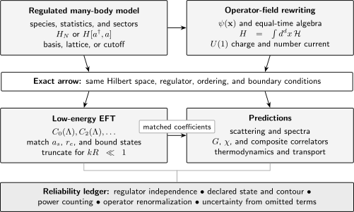
A regulated many-body Hamiltonian and its operator-field form can be exactly equivalent. Replacing short-range dynamics by local operators is an EFT step: the cutoff-dependent coefficients must be matched to scattering or microscopic data before correlators and thermodynamics become regulator-independent predictions.

From a Spatial Lattice to a Continuum Field

A lattice is both a physical model and a possible ultraviolet regulator. Consider a hypercubic Bose–Hubbard discretization with lattice spacing $a_{\mathrm L}$:

$$\begin{aligned} H_{\mathrm L} &= -t_{\mathrm h} \sum_{\langle ij\rangle} \left( a_i^\dagger a_j + a_j^\dagger a_i \right) \\ &\quad+ 2dt_{\mathrm h} \sum_i n_i + \frac{U}{2} \sum_i n_i(n_i-1). \end{aligned}$$

The one-particle dispersion measured from the band minimum is

$$\epsilon_{\mathrm L}(\mathbf k) = 2t_{\mathrm h} \sum_{\ell=1}^{d} \left[ 1-\cos(k_\ell a_{\mathrm L}) \right].$$

For $|\mathbf k|a_{\mathrm L}\ll1$,

$$\epsilon_{\mathrm L}(\mathbf k) = t_{\mathrm h}a_{\mathrm L}^2\mathbf k^2 + \mathcal O(k^4a_{\mathrm L}^4).$$

The continuum identifications are

$$\begin{aligned} a_i &\simeq a_{\mathrm L}^{d/2} \psi(\mathbf x_i), \\ t_{\mathrm h} &= \frac{\hbar^2} {2ma_{\mathrm L}^2}, \\ g_0 &\simeq Ua_{\mathrm L}^{d}. \end{aligned}$$

The first relation preserves

$$\sum_i n_i \simeq \int d^d x\, \psi^\dagger\psi.$$

The last relation is a bare tree-level identification. Quantitative continuum scattering requires matching $U$ at finite $a_{\mathrm L}$ to $a_s$ or another physical datum. The lattice cutoff is of order $\pi/a_{\mathrm L}$, and lattice artifacts appear through higher spatial derivatives.

Taking $a_{\mathrm L}\to0$ is not the same as merely considering long wavelengths in a fixed crystal. A condensed-matter lattice may be physical and retain band structure, Umklapp processes, and only discrete translations. A regulator lattice is removed while selected observables and renormalized parameters are held fixed.

Correlation Functions Are the Observable Language

The field operator itself is not usually measured directly. Experiments and calculations access correlations and responses built from it.

The equal-time one-body density matrix is

$$\rho_1(\mathbf x,\mathbf y) = \left\langle \psi^\dagger(\mathbf y) \psi(\mathbf x) \right\rangle.$$

For a homogeneous system, the momentum distribution is

$$n(\mathbf k) = \int d^d r\, e^{-i\mathbf k\cdot\mathbf r} \left\langle \psi^\dagger(\mathbf r) \psi(\mathbf0) \right\rangle.$$

Density response is controlled by

$$\chi_{nn}^R(t,\mathbf x) = -\frac{i}{\hbar} \Theta(t) \left\langle [n(t,\mathbf x),n(0,\mathbf0)] \right\rangle.$$

Pairing is probed by correlators of a composite field such as

$$\Delta(\mathbf x) = \psi_\downarrow(\mathbf x) \psi_\uparrow(\mathbf x).$$

The single-particle propagator, density response, pair susceptibility, current correlator, and higher-point functions answer different questions. A pole in one channel need not appear in another, and a field redefinition can alter off-shell Green functions without changing scattering amplitudes.

Sources organize these observables. Schematically,

$$Z[J] = \left\langle \mathcal T \exp \left[ \frac{i}{\hbar} \int dt\,d^d x\, J\,\mathcal O \right] \right\rangle.$$

Functional derivatives insert $\mathcal O$. Coupling scalar and vector sources to $n$ and $\mathbf j_N$ makes number-conservation Ward identities manifest. The state, contour, ordering, normalization, and regulator remain part of the definition of $Z[J]$.

Composite operators can require their own renormalization. For example, the short-distance pair density in a contact Fermi gas is related to Tan’s contact only after the cutoff dependence of the local product is combined with that of the coupling. Renormalizing the Hamiltonian does not automatically make every local operator finite.

Bosonic Functional Variables and the Mean-Field Limit

For an equilibrium trace, bosonic coherent states lead formally to

$$Z = \int_{\mathrm{periodic}} \mathcal D\psi^* \mathcal D\psi\, e^{-S_E/\hbar},$$

with

$$\begin{aligned} S_E &= \int_0^{\beta\hbar} d\tau \int d^d x\, \Bigg[ \hbar\psi^*\partial_\tau\psi \\ &\qquad+ \frac{\hbar^2}{2m} |\nabla\psi|^2 - \mu|\psi|^2 + \frac{g_0}{2}|\psi|^4 \Bigg]. \end{aligned}$$

Here $\psi$ is a periodic complex integration variable. For fermions, the variables are Grassmann valued and antiperiodic. The continuum expression is shorthand for a regulated time-sliced construction with a declared operator symbol.

A stationary complex field $\Phi$ obeys

$$i\hbar\partial_t\Phi = \left[ -\frac{\hbar^2\nabla^2}{2m} + V + g_R|\Phi|^2 \right]\Phi.$$

This is the Gross–Pitaevskii equation for a weak dilute Bose gas under its usual assumptions. It is not the exact operator equation with $\psi^\dagger\psi\psi$ replaced freely by $|\langle\psi\rangle|^2\langle\psi\rangle$. The replacement is controlled by condensate occupation, diluteness, dimensionality, and the observable and time scale under study.

Three Representative Theories

Dilute Three-Dimensional Bose Gas

For number density $n$ and positive scattering length $a_s$, the dilute parameter is

$$n a_s^3 \ll 1.$$

At leading order,

$$\frac{E}{V} = \frac{g_Rn^2}{2}, \qquad g_R = \frac{4\pi\hbar^2a_s}{m}.$$

Quantum fluctuations produce the Lee–Huang–Yang correction, whose relative size is proportional to $\sqrt{na_s^3}$. The field theory separates universal low-energy dependence on $a_s$ from short-distance corrections involving effective range and higher-body operators. Bogoliubov Theory owns the fluctuation spectrum and quasiparticle transformation.

One-Dimensional Contact Bosons

The Lieb–Liniger Hamiltonian is

$$\begin{aligned} H &= \int dx\, \Bigg[ \frac{\hbar^2}{2m} \partial_x\psi^\dagger \partial_x\psi \\ &\qquad+ \frac{g_{\mathrm{1D}}}{2} \psi^\dagger\psi^\dagger\psi\psi \Bigg]. \end{aligned}$$

At density $n$, its dimensionless coupling is

$$\gamma = \frac{mg_{\mathrm{1D}}} {\hbar^2n}.$$

The same local field Hamiltonian covers weakly interacting bosons $\gamma\ll1$ and approaches the strongly correlated Tonks–Girardeau regime as $\gamma\to\infty$. The existence of one compact field expression does not imply that perturbation theory about $g_{\mathrm{1D}}=0$ works across both regimes.

Lieb–Liniger Model Preview owns the factor-of-two coupling dictionary, cusp condition, finite-volume Bethe equations, exact-status map, and two-boson ring benchmark. This page owns why the same operator is a nonrelativistic field theory and how its coupling fits the dimensional EFT discussion.

Two-Component Fermi Gas

A minimal zero-range theory is

$$\begin{aligned} \mathcal L &= \sum_{\sigma=\uparrow,\downarrow} \psi_\sigma^\dagger \left( i\hbar\partial_t + \frac{\hbar^2\nabla^2}{2m} + \mu \right) \psi_\sigma \\ &\quad- g_0\, \psi_\uparrow^\dagger \psi_\downarrow^\dagger \psi_\downarrow \psi_\uparrow. \end{aligned}$$

At unitarity,

$$a_s^{-1} = 0, \qquad k_FR \ll 1.$$

The zero-range theory has no two-body length scale, but the many-body density introduces $k_F^{-1}$. Dimensional analysis and nonrelativistic conformal symmetry constrain observables, yet they do not determine all dimensionless many-body constants. The strongly coupled ground-state energy, pairing gap, and transport coefficients require nonperturbative input.

Exact Rewriting Versus Effective Approximation

The same notation can describe steps with very different status.

Operation	Status	Required check
mode expansion in a complete regulated basis	exact change of representation	basis completeness and field algebra
restriction to a fixed-$N$ sector	exact projection if $[H,N]=0$	sector and boundary conditions
replacing $U(r)$ by $g_0\delta^{(d)}(r)$	EFT truncation	$kR\ll1$ and scattering-data matching
removing a cutoff	continuum limit	regulator-independent observables
replacing $\widehat\psi$ by $\Phi$	saddle or mean-field approximation	control parameter and fluctuation test
integrating out a gapped mode	effective theory	energy separation and induced operators
retaining only particles from a relativistic field	nonrelativistic expansion	$E_{\mathrm{kin}}\ll mc^2$ and suppressed pair creation

An approximation can be excellent while the underlying field representation is exact, or a field representation can be exact while a chosen perturbation series is uncontrolled. These are independent judgments.

Nonrelativistic Limit of a Relativistic Field

The reverse bridge starts from relativistic QFT and isolates modes whose kinetic energies are small compared with the rest energy. Set $\hbar=c=1$ in this subsection. A complex relativistic scalar can be decomposed schematically as

$$\begin{aligned} \Phi(\mathbf x,t) &= \frac{1}{\sqrt{2m}} \Bigg[ e^{-imt}\psi(\mathbf x,t) \\ &\qquad+ e^{+imt}\chi^\dagger(\mathbf x,t) \Bigg]. \end{aligned}$$

The slowly varying field $\psi$ annihilates particles and $\chi$ annihilates antiparticles. At external energies and momenta satisfying

$$|E-m| \ll m, \qquad |\mathbf p| \ll m,$$

antiparticle production is kinematically suppressed. Integrating out the antiparticle sector and removing rapidly oscillating terms yields

$$\begin{aligned} \mathcal L_{\mathrm{NR}} &= i\psi^\dagger\partial_t\psi - \frac{|\nabla\psi|^2}{2m} \\ &\quad- \frac{C_0}{2} (\psi^\dagger\psi)^2 + \cdots. \end{aligned}$$

The ellipsis includes relativistic corrections such as higher spatial derivatives and number-changing operators allowed by the underlying theory. For one particle,

$$\sqrt{m^2+\mathbf p^2}-m = \frac{\mathbf p^2}{2m} - \frac{\mathbf p^4}{8m^3} + \cdots.$$

This derivation explains why a nonrelativistic theory can possess an emergent particle-number symmetry even when the relativistic parent does not conserve particle number separately. For a complex scalar, the exact relativistic $U(1)$ charge counts particles minus antiparticles; within the low-energy particle sector it reduces to particle number. A real scalar has no exact $U(1)$ charge, so number conservation in its nonrelativistic EFT is only approximate.

The nonrelativistic limit is not obtained by setting $c=\infty$ inside final relativistic formulas without reorganizing fields, phases, normalization, and operators. Matching determines the coefficients of the resulting EFT.

A Reliability Workflow

Before using a nonrelativistic field theory, record:

1. Degrees of freedom. Species, masses, internal labels, and statistics.
2. Hilbert space. Fixed number sector, Fock space, or grand-canonical ensemble.
3. Symmetries. Global charges, spatial symmetries, time reversal, and any explicit breaking by traps, lattices, or sources.
4. Regulator. Momentum cutoff, lattice spacing, finite basis, dimensional regularization, or another prescription.
5. Operator basis. All local terms required to the intended order.
6. Matching data. Scattering length, effective range, bound-state energy, or microscopic matrix elements.
7. State and contour. Vacuum, ground state, thermal state, or nonequilibrium density operator.
8. Expansion parameter. Diluteness, weak coupling, large component number, derivative order, or scale separation.
9. Observable renormalization. Especially for local composite operators.
10. Stability and limits. Volume, density, cutoff, and long-time order of limits.

A calculation is not reproducible if it quotes only a formal action but omits the regulator, matching prescription, state, and observable definition.

Common Mistakes

1. Calling the field a many-particle wavefunction. It is an operator-valued distribution or a functional-integration coordinate.
2. Equating field notation with relativistic QFT. Nonrelativistic theories have a preferred time and usually Galilean or lattice kinematics.
3. Treating $g_0$ as an observable. A bare contact coupling depends on the regulator.
4. Using $g_R=4\pi\hbar^2a_s/m$ inside divergent loops as though it were bare. Matching and loop regularization must use one scheme consistently.
5. Copying the three-dimensional contact formula into one or two dimensions. Low-energy scattering and running are dimension dependent.
6. Ignoring Pauli antisymmetry. Identical fermions have no local same-component $s$-wave contact interaction.
7. Assuming number conservation means fixed particle number. It means that number sectors do not mix under the Hamiltonian.
8. Confusing chemical potential with explicit number violation. The term $-\mu N$ commutes with $N$.
9. Forgetting that a lattice breaks Galilean boosts. A quadratic band minimum is only a low-momentum approximation.
10. Reading the action without a contour prescription. Retarded, time-ordered, Matsubara, and Schwinger–Keldysh propagators are not interchangeable.
11. Replacing an operator by a saddle field without naming an approximation. Mean-field factorization has a domain of validity.
12. Renormalizing couplings but not composite observables. Coincident-point products can need additional subtractions.
13. Using tree-level power counting at the wrong fixed point. Vacuum, resonance, Fermi-surface, and Goldstone scaling differ.
14. Assuming a zero-range attractive boson model is stable at all densities. Three-body and finite-range physics can become essential.
15. Taking the continuum limit without a matching trajectory. Sending a cutoff to infinity while holding a bare coupling fixed usually changes the physics.

Connections

• Occupation-Number Representation supplies the Fock-space sectors on which the fields act.
• Normal Ordering in Many-Body QM explains reference states and contractions.
• Diagrammatic Methods Preview organizes propagators and vertices into controlled expansions.
• Linear Response and the Kubo Formula connects retarded correlators to measured response.
• Path Integrals for Statistical Mechanics develops thermal traces and imaginary time.
• Path Integrals for Many-Body Systems compares fixed-$N$ worldlines, coherent fields, and lattice-basis histories.
• Coherent-State Path Integrals derives the first-order field term from coherent-state overlap geometry.
• Sources to Generating Functionals develops source derivatives and connected correlators.
• Renormalization Group Preview develops scale-dependent couplings and fixed points.
• Second Quantization: Bridge to QFT compares fixed-particle and Fock-space descriptions.
• QFT Bridge Reference maps the continuation to relativistic fields.

References

1. A. L. Fetter and J. D. Walecka, Quantum Theory of Many-Particle Systems, Dover (2003 reprint) – operator fields, propagators, and many-body perturbation theory.
2. J. W. Negele and H. Orland, Quantum Many-Particle Systems, CRC Press (2018 reissue) – second-quantized actions, coherent-state integrals, and finite-density methods.
3. A. Altland and B. Simons, Condensed Matter Field Theory, Cambridge University Press (2010) – nonrelativistic fields, symmetries, functional methods, and effective theories.
4. D. B. Kaplan, M. J. Savage, and M. B. Wise, “A New Expansion for Nucleon–Nucleon Interactions”, Physics Letters B 424, 390–396 (1998) – contact-EFT power counting and nonperturbative scattering.
5. H.-W. Hammer and R. J. Furnstahl, “Effective Field Theory for Dilute Fermi Systems”, Nuclear Physics A 678, 277–294 (2000) – EFT matching and finite-density expansion.
6. E. Braaten and H.-W. Hammer, “Universality in Few-Body Systems with Large Scattering Length”, Physics Reports 428, 259–390 (2006) – zero-range universality, renormalization, and the three-body parameter.
7. T. D. Lee, K. Huang, and C. N. Yang, “Eigenvalues and Eigenfunctions of a Bose System of Hard Spheres and Its Low-Temperature Properties”, Physical Review 106, 1135–1145 (1957) – dilute Bose-gas expansion and the leading quantum correction.
8. J. O. Andersen, “Theory of the Weakly Interacting Bose Gas”, Reviews of Modern Physics 76, 599–639 (2004) – effective-field-theory treatment of dilute Bose gases.
9. E. H. Lieb and W. Liniger, “Exact Analysis of an Interacting Bose Gas. I. The General Solution and the Ground State”, Physical Review 130, 1605–1616 (1963) – exact one-dimensional contact-boson theory.
10. D. T. Son and M. Wingate, “General Coordinate Invariance and Conformal Invariance in Nonrelativistic Physics: Unitary Fermi Gas”, Annals of Physics 321, 197–224 (2006) – symmetry constraints and effective theory at unitarity.
11. S. Tan, “Energetics of a Strongly Correlated Fermi Gas”, Annals of Physics 323, 2952–2970 (2008) – universal relations and the renormalized short-distance contact.
12. M. H. Namjoo, A. H. Guth, and D. I. Kaiser, “Relativistic Corrections to Nonrelativistic Effective Field Theories”, Physical Review D 98, 016011 (2018) – systematic low-energy reduction of relativistic scalar theories.

Exercises

1. Sector Equivalence for a One-Body Operator

Let

$$H_1 = \int d^d x\, \psi^\dagger(\mathbf x) h(\mathbf x) \psi(\mathbf x).$$

Define

$$\begin{aligned} X_N &\equiv (\mathbf x_1,\ldots,\mathbf x_N), \\ dX_N &\equiv \prod_{r=1}^{N}d^d x_r. \end{aligned}$$

For the normalized $N$-particle state

$$\begin{aligned} |\Psi_N\rangle &= \frac{1}{\sqrt{N!}} \int dX_N\, \Psi_N(X_N) \\ &\quad\times \prod_{j=1}^{N} \psi^\dagger(\mathbf x_j) |0\rangle, \end{aligned}$$

show that $H_1$ acts as $\sum_{j=1}^{N}h_j$ on $\Psi_N$.

Solution

Commute $\psi(\mathbf x)$ through the product of creation fields. Each commutation or anticommutation produces one delta distribution:

$$\begin{aligned} & \psi(\mathbf x) \prod_{j=1}^{N} \psi^\dagger(\mathbf x_j)|0\rangle \\ &\quad= \sum_{\ell=1}^{N} \eta^{\ell-1} \delta^{(d)}(\mathbf x-\mathbf x_\ell) \\ &\qquad\times \prod_{j\ne\ell} \psi^\dagger(\mathbf x_j)|0\rangle, \end{aligned}$$

where $\eta=+1$ for bosons and $\eta=-1$ for fermions, with the remaining creation operators kept in their original order. The exchange symmetry of $\Psi_N$ cancels the corresponding fermionic reorder signs. Acting with $h(\mathbf x)$ and then recreating a particle at $\mathbf x$ gives

$$H_1|\Psi_N\rangle \longleftrightarrow \left( \sum_{\ell=1}^{N}h_\ell \right) \Psi_N.$$

Thus the field operator is exactly the familiar sum of one-particle operators inside the fixed-$N$ sector.

2. Derive the Number Current

Starting from

$$i\hbar\partial_t\psi = \left[ -\frac{\hbar^2\nabla^2}{2m} + V + g_0\psi^\dagger\psi \right]\psi,$$

derive the continuity equation for $n=\psi^\dagger\psi$.

Solution

The adjoint equation is

$$\begin{aligned} -i\hbar\partial_t\psi^\dagger &= -\frac{\hbar^2}{2m} \nabla^2\psi^\dagger + V\psi^\dagger \\ &\quad+ g_0\psi^\dagger\psi^\dagger\psi. \end{aligned}$$

Use

$$\partial_t n = (\partial_t\psi^\dagger)\psi + \psi^\dagger(\partial_t\psi).$$

The real potential and local interaction terms cancel between the two contributions. The kinetic terms give

$$\begin{aligned} \partial_t n &= -\frac{\hbar}{2mi} \left[ \psi^\dagger\nabla^2\psi - (\nabla^2\psi^\dagger)\psi \right] \\ &= -\nabla\mathbin{\cdot}\mathbf j_N, \\ \mathbf j_N &= \frac{\hbar}{2mi} \left[ \psi^\dagger\nabla\psi - (\nabla\psi^\dagger)\psi \right]. \end{aligned}$$

The expression in braces is $\mathbf j_N$, so

$$\partial_t n+\nabla\mathbin{\cdot}\mathbf j_N=0.$$

3. Check the Galilean Boost Phase

Let $\psi$ solve the free Schrödinger equation. Verify that

$$\psi_{\mathbf v}(\mathbf x,t) = e^{im(\mathbf v\cdot\mathbf x-\mathbf v^2t/2)/\hbar} \psi(\mathbf x-\mathbf vt,t)$$

is also a solution, and find its current.

Solution

Write

$$\begin{aligned} \theta(\mathbf x,t) &= \frac{m}{\hbar} \left( \mathbf v\mathbin{\cdot}\mathbf x - \frac{\mathbf v^2t}{2} \right), \\ \mathbf y &= \mathbf x-\mathbf vt. \end{aligned}$$

Then

$$\begin{aligned} \partial_t\psi_{\mathbf v} &= e^{i\theta} \Bigg[ -\frac{im\mathbf v^2}{2\hbar}\psi \\ &\qquad- \mathbf v\mathbin{\cdot}\nabla_{\mathbf y}\psi + \partial_t\psi \Bigg], \\ \nabla_{\mathbf x}\psi_{\mathbf v} &= e^{i\theta} \left[ \frac{im\mathbf v}{\hbar}\psi + \nabla_{\mathbf y}\psi \right]. \end{aligned}$$

Substituting these expressions into $i\hbar\partial_t\psi_{\mathbf v} =-\hbar^2\nabla^2\psi_{\mathbf v}/(2m)$ cancels the terms linear and quadratic in $\mathbf v$, leaving the original equation for $\psi$.

Using the transformed gradient in the current gives

$$\mathbf j_{N,\mathbf v}(\mathbf x,t) = \mathbf j_N(\mathbf y,t) + \mathbf v\,n(\mathbf y,t).$$

The extra term is the convective transport of number density.

4. Determine the Contact Coupling Dimension

Use $z=2$ scaling to derive the field dimension and the scaling of a quartic contact coupling in $d$ dimensions.

Solution

Under

$$\mathbf x\to b\mathbf x, \qquad t\to b^2t,$$

the measure scales as $b^{d+2}$. If $\psi\to b^{-\Delta_\psi}\psi$, the term

$$\int dt\,d^d x\, \psi^\dagger i\hbar\partial_t\psi$$

scales as $b^{d+2-2\Delta_\psi-2}$. Invariance requires

$$\Delta_\psi = \frac d2.$$

The quartic operator contributes $b^{-2d}$, so

$$\int dt\,d^d x\, g(\psi^\dagger\psi)^2$$

scales with $g\,b^{2-d}$. Therefore

$$g' = b^{2-d}g.$$

It is relevant for $d<2$, marginal at $d=2$, and irrelevant for $d>2$ at the Gaussian vacuum fixed point.

5. Match a Sharp-Cutoff Contact Coupling

At zero energy, show that

$$\Pi_\Lambda(0) = -\frac{m\Lambda}{2\pi^2\hbar^2}.$$

Then impose $T(0)=4\pi\hbar^2a_s/m$ to obtain the running of $g_0(\Lambda)$.

Solution

At $E=0$,

$$\begin{aligned} \Pi_\Lambda(0) &= -\frac{m}{\hbar^2} \int_{|\mathbf q|<\Lambda} \frac{d^3q}{(2\pi)^3} \frac{1}{\mathbf q^2} \\ &= -\frac{m}{\hbar^2} \frac{4\pi}{(2\pi)^3} \int_0^\Lambda dq \\ &= -\frac{m\Lambda}{2\pi^2\hbar^2}. \end{aligned}$$

Since

$$T(0)^{-1} = g_0(\Lambda)^{-1} - \Pi_\Lambda(0),$$

matching gives

$$\frac{m}{4\pi\hbar^2a_s} = \frac{1}{g_0(\Lambda)} + \frac{m\Lambda}{2\pi^2\hbar^2}.$$

Hence

$$\frac{1}{g_0(\Lambda)} = \frac{m}{4\pi\hbar^2a_s} - \frac{m\Lambda}{2\pi^2\hbar^2}.$$

The cutoff dependence of the bare coupling cancels that of the loop integral.

6. Recover the Continuum Dispersion from a Lattice

Expand the hypercubic lattice dispersion

$$\epsilon_{\mathrm L}(\mathbf k) = 2t_{\mathrm h} \sum_{\ell=1}^{d} \left[ 1-\cos(k_\ell a_{\mathrm L}) \right]$$

through order $k^4$ and identify the continuum mass.

Solution

Use

$$1-\cos x = \frac{x^2}{2} - \frac{x^4}{24} + \mathcal O(x^6).$$

Then

$$\begin{aligned} \epsilon_{\mathrm L}(\mathbf k) &= t_{\mathrm h}a_{\mathrm L}^2 \mathbf k^2 \\ &\quad- \frac{t_{\mathrm h}a_{\mathrm L}^4}{12} \sum_{\ell=1}^{d}k_\ell^4 + \mathcal O(k^6a_{\mathrm L}^6). \end{aligned}$$

Matching the leading term to $\hbar^2\mathbf k^2/(2m)$ gives

$$t_{\mathrm h} = \frac{\hbar^2}{2ma_{\mathrm L}^2}.$$

The quartic correction is anisotropic because the lattice has only hypercubic, not continuous rotational, symmetry. It vanishes relative to the quadratic term when $|\mathbf k|a_{\mathrm L}\to0$.

7. Uniform Bose Saddle

For $V=0$ and $g_R>0$, find a homogeneous stationary solution of the Gross–Pitaevskii equation with density $n_0$. Explain which conclusion is exact and which is mean field.

Solution

Take

$$\Phi(t) = \sqrt{n_0}\, e^{-i\mu_{\mathrm B}t/\hbar}.$$

Substitution into

$$i\hbar\partial_t\Phi = g_R|\Phi|^2\Phi$$

gives

$$\mu_{\mathrm B} = g_Rn_0.$$

The operator Hamiltonian and its $U(1)$ symmetry are exact within the regulated contact model. Replacing the operator field by $\Phi$ and factorizing the quartic interaction is the mean-field approximation. The relation $\mu_{\mathrm B}=g_Rn_0$ is its leading dilute-gas prediction; fluctuation corrections modify it.

8. Number-Charged Expectation Values

Suppose

$$[H,N]=0, \qquad [\rho,N]=0,$$

and an operator $O_q$ obeys

$$[N,O_q] = -qO_q.$$

Show that $\operatorname{Tr}(\rho O_q)=0$ for $q\ne0$. Why can a symmetry-breaking treatment nevertheless use $\langle\psi\rangle\ne0$?

Solution

Let

$$U(\alpha) = e^{i\alpha N}.$$

The commutator implies

$$U(\alpha)O_qU^\dagger(\alpha) = e^{-iq\alpha}O_q.$$

Because $\rho$ commutes with $U(\alpha)$ and the trace is cyclic,

$$\begin{aligned} \operatorname{Tr}(\rho O_q) &= \operatorname{Tr} \left[ \rho U(\alpha)O_qU^\dagger(\alpha) \right] \\ &= e^{-iq\alpha} \operatorname{Tr}(\rho O_q). \end{aligned}$$

For $q\ne0$, one can choose $\alpha$ so that the phase is not one. The only consistent result is

$$\operatorname{Tr}(\rho O_q) = 0.$$

A symmetry-breaking treatment introduces a small charge-selecting source, takes the thermodynamic limit before removing it, or works in a phase-fixed effective description. Then $\langle\psi\rangle$ can serve as an order parameter even though a finite, exactly number-symmetric density operator has zero one-point function. Number-conserving observables and correlation functions remain available in either formulation.