Path Integrals for Statistical Mechanics

A thermal path integral represents a quantum partition function as a sum over configurations that close around a compact imaginary-time direction.

For a particle with

$$H = \frac{P^2}{2m} + V(Q),$$

the canonical partition function has the formal representation

$$\begin{aligned} Z(\beta) &= \operatorname{Tr}e^{-\beta H} \\ &= \int_{q(\beta\hbar)=q(0)} \mathcal Dq\, e^{-S_{\mathrm E}[q]/\hbar}, \end{aligned}$$

with Euclidean action

$$S_{\mathrm E}[q] = \int_0^{\beta\hbar} d\tau\, \left[ \frac{m}{2}\dot q(\tau)^2 + V\big(q(\tau)\big) \right].$$

Three pieces of this formula carry most of its meaning:

1. the trace identifies the two endpoints, so the paths are closed;
2. the circumference of the imaginary-time circle is $\beta\hbar$;
3. the weight is $e^{-S_{\mathrm E}/\hbar}$, not the real-time phase $e^{iS/\hbar}$.

The continuum expression is compact, but its measure and boundary condition are defined by a regulated time-sliced limit. That finite approximation is where normalization, exchange sectors, discretization error, and numerical algorithms become concrete.

Canonical Scope

This page is the canonical home for:

• deriving a closed coordinate path integral from $\operatorname{Tr}e^{-\beta H}$;
• the cyclic finite-slice measure and its continuum limit;
• the imaginary-time circle and its coordinate boundary conditions;
• closure up to a permutation for identical particles;
• the ring-polymer representation of a quantum partition function;
• coordinate insertions and source-dependent thermal functionals;
• the periodic-mode determinant of the thermal harmonic oscillator;
• discretization, sampling, and sign-problem diagnostics.

Neighboring pages retain distinct ownership:

• Partition Functions owns basis-independent traces, thermodynamic derivatives, convergence, factorization, and ensemble bookkeeping.
• Imaginary Time owns the operator semigroup, spectral damping, open-versus-closed operator dictionary, and projection limit.
• Euclidean and Imaginary-Time Path Integrals owns Wick rotation, open Euclidean kernels, elementary time slicing, and ground-state projection.
• Matsubara Formalism Preview owns the compact-time Fourier workflow and frequency-sum techniques.
• Coherent-State Path Integrals Preview owns bosonic and fermionic Fock-space traces, Grassmann labels, determinant checks, and ordering caveats.
• Thermal Green Functions owns imaginary-time ordering, equal-time jumps, and free thermal propagators.
• From Euclidean Time to Euclidean QFT owns the promotion from particle coordinates to fields, reflection positivity, and Lorentzian reconstruction.

Coherent-State Path Integrals Preview changes both the integration variables and the boundary-condition logic. This page therefore keeps its main derivation in ordinary first-quantized coordinates.

Assumptions and Conventions

Unless stated otherwise:

1. $H=P^2/(2m)+V(Q)$ is self-adjoint and bounded below;

2. $e^{-\beta H}$ is trace class, or the system is placed in a finite box before a thermodynamic limit is taken;

3. $\beta=(k_{\mathrm B}T)^{-1}$;

4. $\hbar$ is kept explicit;

5. imaginary time is denoted by $\tau$ and has units of time;

6. the thermal circumference is

   $$L_\tau = \beta\hbar;$$

7. $M$ is the number of imaginary-time slices, with

   $$\epsilon_\tau = \frac{L_\tau}{M} = \frac{\beta\hbar}{M}.$$

For several coordinates, $q$ becomes a vector and the scalar mass becomes a mass matrix or a list of particle masses. Potentials with singularities, magnetic terms, constrained configuration spaces, or velocity dependence require refinements of the elementary short-time kernel.

From a Trace to a Closed Path

Begin with the coordinate-space trace:

$$Z(\beta) = \int dq_0\, \langle q_0| e^{-\beta H} |q_0\rangle.$$

The repeated coordinate is not decorative. It is the trace condition.

Write the Gibbs operator as $M$ short imaginary-time steps:

$$e^{-\beta H} = \left( e^{-\epsilon_\tau H/\hbar} \right)^M.$$

Insert $M-1$ coordinate resolutions of the identity,

$$I = \int dq_j\, |q_j\rangle\langle q_j|,$$

between successive factors. The result is

$$\begin{aligned} Z_M &= \int \prod_{j=0}^{M-1}dq_j \prod_{j=0}^{M-1} \langle q_{j+1}| e^{-\epsilon_\tau H/\hbar} |q_j\rangle, \\ q_M &= q_0. \end{aligned}$$

Every coordinate is integrated, including the coordinate at which the trace was written. There are no externally fixed endpoints. Relabeling the beads

$$q_j \longmapsto q_{j+r\ {\rm mod}\ M}$$

leaves the exact cyclic expression invariant. This discrete symmetry becomes translation around the thermal circle in the continuum limit.

The Product Formula

Let

$$T = \frac{P^2}{2m}, \qquad H=T+V.$$

Because $T$ and $V$ generally do not commute, the short-time operator cannot simply be split as an exact product. The Lie–Trotter formula gives

$$e^{-\epsilon_\tau(T+V)/\hbar} = e^{-\epsilon_\tau T/\hbar} e^{-\epsilon_\tau V/\hbar} + \mathcal O(\epsilon_\tau^2)$$

at the local operator level under suitable domain and commutator assumptions. Multiplying $M=L_\tau/\epsilon_\tau$ steps produces a primitive global error of order $\epsilon_\tau$.

A symmetric factorization is usually preferable:

$$\begin{aligned} e^{-\epsilon_\tau(T+V)/\hbar} &= e^{-\epsilon_\tau V/(2\hbar)} e^{-\epsilon_\tau T/\hbar} e^{-\epsilon_\tau V/(2\hbar)} \\ &\quad + \mathcal O(\epsilon_\tau^3). \end{aligned}$$

When the required commutators are controlled, the accumulated error is then $\mathcal O(\epsilon_\tau^2)$. Singular interactions can invalidate a naive pointwise error estimate even when an operator product formula still converges. Numerical work should verify the observed continuum scaling.

The Short-Time Coordinate Kernel

Define the short-time normalization

$$\mathcal N_{\epsilon_\tau} = \left( \frac{m}{2\pi\hbar\epsilon_\tau} \right)^{1/2}.$$

The kinetic factor then has the exact Gaussian kernel

$$\begin{aligned} K_0 &\equiv \langle q'\rvert e^{-\epsilon_\tau P^2/(2m\hbar)} \lvert q\rangle \\ K_0 &= \mathcal N_{\epsilon_\tau} \exp\left[ -\frac{m}{2\hbar\epsilon_\tau} (q'-q)^2 \right]. \end{aligned}$$

For compact notation, set

$$\begin{aligned} \delta q_j &= q_{j+1}-q_j, \\ \overline V_j &= \frac{V(q_{j+1})+V(q_j)}{2}. \end{aligned}$$

Using the symmetric factorization gives

$$\begin{aligned} K_j &\equiv \langle q_{j+1}\rvert e^{-\epsilon_\tau H/\hbar} \lvert q_j\rangle, \\ K_j &\simeq \mathcal N_{\epsilon_\tau} \\ &\quad\times \exp\left[ -\frac{m(\delta q_j)^2} {2\hbar\epsilon_\tau} \right] \\ &\quad\times \exp\left[ -\frac{\epsilon_\tau}{\hbar} \overline V_j \right]. \end{aligned}$$

In a cyclic product, every potential value appears in two adjacent half steps. Introduce

$$\begin{aligned} \Delta_\tau q_j &= \frac{q_{j+1}-q_j}{\epsilon_\tau}, \\ \mathcal L_j &= \frac{m}{2} (\Delta_\tau q_j)^2 + V(q_j), \\ S_{{\mathrm E},M} &= \epsilon_\tau \sum_{j=0}^{M-1} \mathcal L_j. \end{aligned}$$

The finite-slice partition function is then

$$\begin{aligned} Z_M &= \mathcal N_{\epsilon_\tau}^{\,M} \int \prod_{j=0}^{M-1}dq_j \\ &\quad\times \exp\left[ -\frac{S_{{\mathrm E},M}}{\hbar} \right], \\ q_M &= q_0, \end{aligned}$$

up to the chosen factorization error.

This expression is the operational definition of the coordinate path integral. It specifies:

• the number of integration variables;
• the normalization of the measure;
• the cyclic boundary condition;
• the nearest-neighbor kinetic term;
• the local potential weight;
• the limiting procedure $M\to\infty$.

Dropping the Gaussian prefactor may be harmless in a normalized expectation value whose numerator and denominator use the same measure. It is not harmless for an absolute partition function or free energy.

Continuum Notation

With the discrete action and measure specified above, the time-sliced limit is abbreviated as

$$\begin{aligned} Z &= \lim_{M\to\infty}Z_M \\ &= \int_{\mathrm{periodic}} \mathcal Dq\, e^{-S_{\mathrm E}[q]/\hbar}, \\ q(L_\tau) &= q(0). \end{aligned}$$

The symbol $\mathcal Dq$ is not an infinite-dimensional Lebesgue measure. Its meaning comes from a limiting construction, a mathematically equivalent Wiener-measure formulation where available, or another declared regulator.

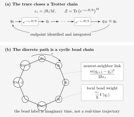
The trace identifies the final coordinate with the initial one and integrates it. After time slicing, the kinetic action couples neighboring beads while the potential acts locally on each bead. The bead index labels imaginary time; it is not a sequence of real-time positions.

The Imaginary-Time Circle

The path lives on

$$\tau \sim \tau+L_\tau, \qquad L_\tau=\beta\hbar.$$

This compact direction has no preferred starting point in an equilibrium trace. For a time-independent Hamiltonian, shifting every insertion by the same imaginary time leaves a thermal correlator unchanged, provided the ordering and wraparound are handled consistently.

Temperature changes the circumference:

• high temperature means a short imaginary-time circle;
• low temperature means a long imaginary-time circle;
• the zero-temperature limit sends $L_\tau\to\infty$.

Compactness produces discrete Fourier modes. A real periodic coordinate may be expanded as

$$q(\tau) = \sum_{\ell\in\mathbb Z} q_\ell e^{i\nu_\ell\tau},$$

where

$$\nu_\ell = \frac{2\pi\ell}{\beta\hbar}, \qquad q_{-\ell}=q_\ell^*.$$

The $\ell=0$ component is the centroid

$$\bar q = \frac{1}{\beta\hbar} \int_0^{\beta\hbar} d\tau\,q(\tau).$$

Nonzero modes describe variation around the circle. They are quantum fluctuation modes in the equilibrium representation, not harmonics of a real-time orbit.

Bosonic and Fermionic Matsubara Frequencies develops the general boundary-condition-to-frequency dictionary.

Boundary Conditions Are Part of the Quantity

Several superficially similar Euclidean constructions compute different objects.

• Open coordinate kernel: fix $q(0)=q_i$ and $q(\tau_f)=q_f$ to compute $\langle q_f\rvert e^{-\tau_fH/\hbar}\lvert q_i\rangle$.
• Coordinate thermal trace: impose $q(L_\tau)=q(0)$ and integrate that coordinate to compute $\operatorname{Tr}e^{-\beta H}$.
• Distinguishable many-particle trace: close every labeled coordinate around the thermal circle.
• Identical-particle trace: close the endpoint configuration up to a permutation, with the statistical weight of that permutation.
• Bosonic coherent-state field: use a periodic field in the thermal functional integral.
• Fermionic coherent-state field: use an antiperiodic Grassmann field in the thermal functional integral.

The last two cases do not mean that an ordinary fermion position coordinate obeys

$$q(\beta\hbar) = -q(0).$$

That statement would confuse first-quantized coordinate paths with fermionic coherent-state variables. In a coordinate worldline formulation, identical-particle statistics enters through permutation sectors and their signs.

Twisted traces provide a useful generalization. If a symmetry operator $U$ is inserted,

$$Z_U = \operatorname{Tr} \left( Ue^{-\beta H} \right),$$

then the path may close with a corresponding twist. The boundary condition must be derived from the trace insertion; it should not be guessed from the particle’s label.

Identical Particles and Permutation Closure

Let

$$\mathbf q = (\mathbf r_1,\ldots,\mathbf r_N)$$

denote a labeled coordinate representative of an $N$-particle configuration. Projection onto the symmetric or antisymmetric Hilbert space gives

$$\begin{aligned} Z_N^{(\pm)} &= \frac{1}{N!} \sum_{P\in S_N} (\pm1)^P \\ &\quad\times \int_{\mathbf q(L_\tau)=P\mathbf q(0)} \mathcal D\mathbf q\, e^{-S_{\mathrm E}[\mathbf q]/\hbar}. \end{aligned}$$

Here:

• every permutation has weight $+1$ for bosons;
• a fermionic permutation has the parity sign $(-1)^P$;
• the factor $1/N!$ compensates for labeled coordinate representatives;
• a permutation cycle joins particle worldlines into a longer exchange loop.

For bosons with a nonnegative coordinate action, exchange sectors enlarge the positive configuration sum. For fermions, even and odd sectors cancel. That cancellation is one origin of the fermion sign problem.

This formula is exact for the canonical trace once spin, internal states, and the interaction are included consistently. It does not imply that particles follow identifiable trajectories. Worldline connectivity is a representation of the trace over the symmetrized or antisymmetrized Hilbert space.

The Symmetrization Postulate owns the Hilbert-space statement behind the permutation projector.

The Ring-Polymer Isomorphism

The finite-slice expression can be rewritten as a classical configurational integral in an enlarged space. Define

$$\beta_M = \frac{\beta}{M}, \qquad \omega_M = \frac{M}{\beta\hbar}.$$

Then

$$\frac{m(q_{j+1}-q_j)^2} {2\hbar\epsilon_\tau} = \beta_M \frac{m\omega_M^2}{2} (q_{j+1}-q_j)^2.$$

Consequently,

$$\begin{aligned} Z_M &= \left( \frac{mM}{2\pi\beta\hbar^2} \right)^{M/2} \int \prod_{j=0}^{M-1}dq_j\, e^{-\beta_M U_M}, \\ U_M &= \sum_{j=0}^{M-1} \left[ \frac{m\omega_M^2}{2} (q_{j+1}-q_j)^2 + V(q_j) \right]. \end{aligned}$$

The quantum particle maps to a cyclic chain of $M$ replicas:

• neighboring replicas are joined by harmonic springs;
• each replica feels the physical potential;
• the centroid is the zero mode of the spring network;
• internal ring modes encode imaginary-time fluctuations.

This is an equilibrium configurational isomorphism. The bead index is not physical time, and a fictitious molecular-dynamics trajectory used to sample the beads is not the quantum particle’s real-time trajectory.

The representation nevertheless has major practical value. Normal-mode and staging transformations can reduce sampling stiffness, path-integral Monte Carlo can sample the equilibrium distribution, and ring-polymer-based approximations can be constructed for selected dynamical questions. Those dynamical approximations require separate justification.

The Classical Limit in the Bead Picture

At fixed $\beta$, the spring frequency grows as $\hbar\to0$:

$$\omega_M = \frac{M}{\beta\hbar} \longrightarrow \infty.$$

The beads collapse toward a common coordinate. The one-slice expression is

$$Z_1 = \left( \frac{m}{2\pi\beta\hbar^2} \right)^{1/2} \int dq\, e^{-\beta V(q)}.$$

This equals the classical phase-space partition function

$$\begin{aligned} Z_{\mathrm{cl}} &= \frac{1}{h} \int dp\,dq\, e^{-\beta[p^2/(2m)+V(q)]} \\ &= \left( \frac{m}{2\pi\beta\hbar^2} \right)^{1/2} \int dq\, e^{-\beta V(q)}. \end{aligned}$$

The equality does not mean $M=1$ is generally an accurate quantum approximation. It identifies the collapsed-bead limit. At finite $\hbar$, convergence requires enough slices to resolve the fastest relevant imaginary-time variation.

Classical Limit of Quantum Statistics develops the separate issues of dilute statistics, exchange suppression, and phase-space counting.

Thermal Observables as Insertions

For a coordinate-diagonal observable $A(Q)$,

$$\langle A\rangle_\beta = \frac{1}{Z} \operatorname{Tr} \left( e^{-\beta H}A \right).$$

Insertion at a particular bead gives

$$\langle A\rangle_{\beta,M} = \frac{1}{Z_M} \int d\mu_M(\mathbf q)\, A(q_j),$$

where $d\mu_M$ denotes the full normalized cyclic weight. Cyclic symmetry permits the lower-variance bead average

$$A_M = \frac{1}{M} \sum_{j=0}^{M-1}A(q_j).$$

For an imaginary-time ordered coordinate correlator,

$$C_{AB}(\tau) = \left\langle \mathcal T_\tau A\big(q(\tau)\big) B\big(q(0)\big) \right\rangle_\beta,$$

the two functions are inserted at the corresponding points of the circle.

Momentum, kinetic energy, and off-diagonal operators are subtler. They act on short-time kernels rather than simply multiplying each bead configuration. Thermodynamic, primitive, virial, and centroid-virial estimators can be algebraically equivalent in the continuum limit while having very different finite-$M$ variance.

A Source-Dependent Functional

Introduce a periodic source $J(\tau)$ and define the source-shifted action

$$S_{{\mathrm E},J}[q] = S_{\mathrm E}[q] - \int_0^{L_\tau} d\tau\, J(\tau)q(\tau).$$

The generating functional is

$$Z[J] = \int_{\mathrm{periodic}} \mathcal Dq\, e^{-S_{{\mathrm E},J}[q]/\hbar}.$$

Then

$$\frac{\delta\ln Z[J]} {\delta J(\tau)} = \frac{1}{\hbar} \langle q(\tau)\rangle_J,$$

and

$$\frac{\delta^2\ln Z[J]} {\delta J(\tau)\delta J(\tau')} = \frac{1}{\hbar^2} \langle q(\tau)q(\tau')\rangle_{J,c}.$$

Functional derivatives therefore generate connected Euclidean correlations. Replacing a finite list of coordinates by a spatial field produces the basic architecture of a statistical field theory. Statistical Field Theory Preview develops its regulated measure, coarse-field weight, and fluctuation integral; From Euclidean Time to Euclidean QFT develops continuum and Lorentzian reconstruction questions specific to Euclidean quantum fields.

Exact Benchmark: The Thermal Harmonic Oscillator

Consider

$$H = \frac{P^2}{2m} + \frac{m\omega^2Q^2}{2}.$$

Its Euclidean action is quadratic:

$$S_{\mathrm E}[q] = \frac{m}{2} \int_0^{\beta\hbar} d\tau\, \left[ \dot q(\tau)^2 + \omega^2q(\tau)^2 \right],$$

with

$$q(\beta\hbar) = q(0).$$

Expand in periodic modes,

$$q(\tau) = \sum_{\ell\in\mathbb Z} q_\ell e^{i\nu_\ell\tau}, \qquad \nu_\ell = \frac{2\pi\ell}{\beta\hbar}.$$

Orthogonality diagonalizes the action:

$$S_{\mathrm E} = \frac{\beta\hbar m}{2} \sum_{\ell\in\mathbb Z} \left( \nu_\ell^2+\omega^2 \right) |q_\ell|^2.$$

The path integral is therefore a product of Gaussian mode integrals. After fixing the absolute normalization by the time-sliced measure, the zero mode and paired nonzero modes give

$$Z_{\mathrm{ho}} = \frac{1}{\beta\hbar\omega} \prod_{\ell=1}^{\infty} \frac{\nu_\ell^2} {\nu_\ell^2+\omega^2}.$$

Let

$$x = \frac{\beta\hbar\omega}{2}.$$

Euler’s product

$$\frac{\sinh x}{x} = \prod_{\ell=1}^{\infty} \left( 1+\frac{x^2}{\pi^2\ell^2} \right)$$

implies

$$\prod_{\ell=1}^{\infty} \frac{\nu_\ell^2} {\nu_\ell^2+\omega^2} = \frac{x}{\sinh x}.$$

Hence

$$Z_{\mathrm{ho}} = \frac{1} {2\sinh(\beta\hbar\omega/2)}.$$

This agrees with the spectral sum

$$\begin{aligned} Z_{\mathrm{ho}} &= \sum_{n=0}^{\infty} e^{-\beta\hbar\omega(n+1/2)} \\ &= \frac{e^{-\beta\hbar\omega/2}} {1-e^{-\beta\hbar\omega}}. \end{aligned}$$

The two derivations organize the same physics differently. The spectral sum resolves energy eigenstates; the path integral resolves periodic imaginary-time modes.

The Quantum Harmonic Oscillator owns the spectrum and stationary-state solution. Harmonic-Oscillator Path Integral owns the real-time and open-kernel Gaussian construction.

Oscillator Checks

High temperature

For $x\ll1$,

$$\sinh x = x+\frac{x^3}{6}+\cdots,$$

so

$$Z_{\mathrm{ho}} = \frac{1}{\beta\hbar\omega} \left[ 1-\frac{(\beta\hbar\omega)^2}{24} +\cdots \right].$$

The leading term is the classical oscillator partition function.

Low temperature

For $x\gg1$,

$$Z_{\mathrm{ho}} = e^{-\beta\hbar\omega/2} \left[ 1+e^{-\beta\hbar\omega} +\cdots \right].$$

The ground-state Boltzmann factor dominates, while excited states are exponentially suppressed.

Internal energy

Differentiation gives

$$\begin{aligned} U &= -\frac{\partial\ln Z_{\mathrm{ho}}} {\partial\beta} \\ &= \frac{\hbar\omega}{2} \coth\left( \frac{\beta\hbar\omega}{2} \right). \end{aligned}$$

Thus

$$U \longrightarrow \begin{cases} k_{\mathrm B}T, & \beta\hbar\omega\ll1, \\ \hbar\omega/2, & \beta\hbar\omega\gg1. \end{cases}$$

Position variance

Differentiating with respect to $\omega^2$ yields

$$\langle Q^2\rangle_\beta = \frac{\hbar}{2m\omega} \coth\left( \frac{\beta\hbar\omega}{2} \right).$$

The centroid mode alone has variance

$$\langle |q_0|^2\rangle = \frac{1}{\beta m\omega^2}.$$

At high temperature this becomes the full classical variance. At low temperature, nonzero imaginary-time modes supply the additional quantum width.

Many Coordinates and Many Particles

For coordinates $\mathbf q$ with positive mass matrix $\mathsf M$,

$$H = \frac{1}{2} \mathbf P^{\mathsf T} \mathsf M^{-1} \mathbf P + V(\mathbf Q),$$

the Euclidean action becomes

$$S_{\mathrm E}[\mathbf q] = \int_0^{\beta\hbar} d\tau\, \left[ \frac{1}{2} \dot{\mathbf q}^{\mathsf T} \mathsf M \dot{\mathbf q} + V(\mathbf q) \right].$$

Each coordinate produces its own cyclic bead chain, while interactions couple coordinates within the same imaginary-time slice. For pair interactions,

$$V(\mathbf q_j) = \sum_a V_{\mathrm{ext}}(\mathbf r_{a,j}) + \sum_{a<b} v(\mathbf r_{a,j}-\mathbf r_{b,j}).$$

The imaginary-time springs connect $(a,j)$ to $(a,j+1)$; physical interactions connect particles at a common slice. Exchange sectors can reconnect worldlines across the thermal boundary.

In a grand-canonical coordinate formulation,

$$\Xi = \sum_{N=0}^{\infty} z^N Z_N, \qquad z=e^{\beta\mu}.$$

Changing particle number is often handled more naturally with worldline updates or coherent-state fields. The finite-$N$ coordinate derivation remains useful because it makes exchange topology explicit.

What the Path Integral Makes Visible

The representation reorganizes equilibrium quantum mechanics in several productive ways.

Quantum fluctuations become geometry in imaginary time

Rapid variation of $q(\tau)$ costs kinetic action. The competition between that stiffness and the potential determines the distribution of closed paths.

Low temperature exposes low-energy structure

As $\beta$ grows, the circle lengthens. Correlations can decay over a larger imaginary-time range, making excitation gaps visible through exponential behavior.

Exchange becomes worldline connectivity

Permutation cycles translate symmetrization into topology of the thermal boundary. Long cycles are especially important in Bose statistics, but their interpretation depends on dimension, interactions, and the observable.

Collective descriptions become natural

Auxiliary fields, order-parameter fields, and density fields can replace or supplement microscopic coordinates. This creates a direct bridge to statistical field theory and saddle-point methods; Landau–Ginzburg Theory Preview develops the resulting static order-parameter functional and its fluctuation integral.

Positivity is conditional

For a distinguishable particle with a real scalar potential, the coordinate weight is nonnegative. Fermionic exchange, magnetic phases, chemical potentials in some field formulations, frustration, and topological terms can make the effective weight signed or complex.

Numerical Workflow

A reliable finite-temperature path-integral calculation should make the following choices explicit.

1. Define the ensemble and regulator

State whether the calculation is canonical or grand canonical, whether volume is finite, and how singular interactions or continuum ultraviolet behavior are regulated.

2. Choose a factorization

Record the primitive, symmetric, pair-action, or higher-order approximation. The formal order alone does not guarantee a smaller error at the accessible slice numbers.

3. Converge the slice number

Repeat the calculation for increasing $M$. For a symmetric action, an extrapolation of the form

$$O_M = O_\infty + \frac{a}{M^2} + \frac{b}{M^4} +\cdots$$

may be appropriate after the asymptotic regime is demonstrated. It should not be assumed from two points.

4. Resolve the fastest scale

For an oscillator, the relevant dimensionless stiffness is $\beta\hbar\omega$. Interacting systems may contain much larger local frequencies than their low-energy collective scale. A slice count adequate for long-distance observables can still underresolve short-range structure.

5. Sample the cyclic modes efficiently

Local bead updates become slow when the springs are stiff. Normal-mode moves, staging transformations, multilevel methods, hybrid Monte Carlo, and problem-specific cluster or worm updates can reduce autocorrelation.

6. Match the estimator to the observable

Coordinate-diagonal averages are straightforward. Kinetic energy, free-energy differences, off-diagonal density matrices, superfluid response, and real-frequency spectra require specialized estimators or additional inference.

7. Quantify signs and phases

If weights are written as

$$w(q) = |w(q)|e^{i\theta(q)},$$

reweighting gives

$$\langle O\rangle_w = \frac{ \langle Oe^{i\theta}\rangle_{|w|} }{ \langle e^{i\theta}\rangle_{|w|} }.$$

An exponentially small denominator produces exponentially poor signal. Reporting only accepted samples or nominal Monte Carlo steps hides this loss of information.

8. Separate statistical and systematic error

Quote Monte Carlo uncertainty, autocorrelation treatment, finite-$M$ error, finite-volume error, model truncation, and any analytic-continuation uncertainty separately.

Discretization and Measure Caveats

The elementary derivation is robust, but several refinements matter in research calculations.

• Singular potentials: Coulomb cores and hard constraints may require exact or improved short-time density matrices.
• Curved configuration spaces: the measure and action can acquire metric determinants and ordering-dependent terms.
• Magnetic fields: vector potentials produce phase-sensitive Euclidean actions; gauge covariance must be preserved.
• Nonlocal interactions: the action can couple different imaginary times rather than remaining bead-local.
• Operator ordering: momentum-dependent Hamiltonians cannot be converted by substituting $p\to m\dot q$ without checking the discretization prescription.
• Thermodynamic limit: a finite-volume trace may exist even when the infinite-volume partition function diverges; intensive limits must be taken after normalization.
• Continuum fields: infinitely many spatial modes introduce a second regulator in addition to the imaginary-time slicing.

The continuum symbol conceals these choices. A trustworthy calculation states them.

Common Mistakes

1. Treating $q(\tau)$ as a measured trajectory. It is an integration variable in an equilibrium representation.
2. Forgetting the endpoint integral. Setting $q_M=q_0$ closes the path; integrating $q_0$ performs the trace.
3. Using a real-time phase. Thermal Euclidean weights are $e^{-S_{\mathrm E}/\hbar}$.
4. Dropping the measure normalization in an absolute $Z$. Free energies depend on it.
5. Calling every coordinate path periodic for identical particles. Exchange sectors close only up to a permutation.
6. Making fermion coordinates antiperiodic. Antiperiodicity belongs to fermionic coherent-state fields; coordinate statistics is implemented by permutation signs.
7. Assuming a Euclidean weight is positive. Fermion signs and complex phases can remain.
8. Equating the ring-polymer sampling time with real time. The sampling dynamics is algorithmic.
9. Taking $M$ large without a convergence study. A large integer is not an error estimate.
10. Ignoring the zero mode. Static and centroid contributions can dominate infrared behavior.
11. Using the oscillator determinant without fixing normalization. Ratios of determinants do not by themselves determine the absolute partition function.
12. Analytically continuing noisy data as a routine Fourier transform. Analytic Continuation explains why the inverse problem is ill-conditioned.

Practical Decision Guide

Use a coordinate thermal path integral when:

• the Hamiltonian has a natural coordinate-space kinetic-plus-potential form;
• equilibrium coordinate observables are central;
• semiclassical saddles or tunneling paths are informative;
• stochastic sampling of a nonnegative or manageable weight is possible;
• exchange can be handled through worldline sectors.

Prefer another representation when:

• a small exact spectrum is already available;
• fermionic cancellation overwhelms coordinate sampling;
• creation and annihilation processes make Fock-space fields more natural;
• the target is genuine real-time nonequilibrium evolution;
• an operator or tensor-network method controls the relevant structure more directly.

The path integral is a representation, not automatically an approximation and not automatically a good numerical method.

Connections

• Finite-Temperature QM Overview places path integrals alongside spectral, operator, and Matsubara methods.
• Imaginary Time supplies the semigroup and trace interpretation before any path-integral representation is chosen.
• Partition Functions develops thermodynamic generation and ensemble structure.
• Thermal Density Operators develops normalization and mixed-state meaning.
• Matsubara Formalism Preview turns compact-time dependence into discrete frequency sums.
• Thermal Green Functions develops ordered operator correlators and their boundary conditions.
• Path Integrals for Many-Body Systems compares coordinate worldlines with Fock-space fields and lattice-basis histories.
• Euclidean and Imaginary-Time Path Integrals develops open kernels, Wick rotation, and projection.
• From Euclidean Time to Euclidean QFT continues from particle paths to regulated field configurations.

References

1. H. F. Trotter, “On the Product of Semi-Groups of Operators”, Proceedings of the American Mathematical Society 10, 545–551 (1959) – operator product formula underlying imaginary-time slicing.
2. M. Kac, “On Distributions of Certain Wiener Functionals”, Transactions of the American Mathematical Society 65, 1–13 (1949) – probabilistic foundation related to the Feynman–Kac representation.
3. R. P. Feynman and A. R. Hibbs, Quantum Mechanics and Path Integrals, McGraw–Hill (1965) – foundational physical treatment of real- and imaginary-time path integrals.
4. L. S. Schulman, Techniques and Applications of Path Integration, Springer (1981) – detailed path-integral methods, kernels, and boundary conditions.
5. D. Chandler and P. G. Wolynes, “Exploiting the Isomorphism between Quantum Theory and Classical Statistical Mechanics of Polyatomic Fluids”, Journal of Chemical Physics 74, 4078–4095 (1981) – ring-polymer isomorphism and molecular applications.
6. D. M. Ceperley, “Path Integrals in the Theory of Condensed Helium”, Reviews of Modern Physics 67, 279–355 (1995) – permutation cycles, estimators, and path-integral Monte Carlo.
7. M. Suzuki, “Generalized Trotter’s Formula and Systematic Approximants of Exponential Operators and Inner Derivations with Applications to Many-Body Problems”, Progress of Theoretical Physics 56, 1454–1469 (1976) – higher-order product formulas.
8. J. W. Negele and H. Orland, Quantum Many-Particle Systems, CRC Press (2018 reissue) – coherent-state functionals, finite-temperature many-body theory, and field-theory methods.

Exercises

1. Trace closure

Starting from

$$Z = \int dq_0\, \langle q_0|e^{-\beta H}|q_0\rangle,$$

insert three short-time factors and the required coordinate identities. Write the complete integral and state the endpoint condition.

Solution

For $M=3$, let

$$\epsilon_\tau = \frac{\beta\hbar}{3}.$$

Then

$$\begin{aligned} Z &= \int dq_0\,dq_1\,dq_2\, \langle q_0| e^{-\epsilon_\tau H/\hbar} |q_2\rangle \\ &\quad\times \langle q_2| e^{-\epsilon_\tau H/\hbar} |q_1\rangle \langle q_1| e^{-\epsilon_\tau H/\hbar} |q_0\rangle. \end{aligned}$$

Equivalently, with $q_3=q_0$,

$$Z = \int \prod_{j=0}^{2}dq_j \prod_{j=0}^{2} \langle q_{j+1}| e^{-\epsilon_\tau H/\hbar} |q_j\rangle.$$

All three coordinates are integrated. The equality $q_3=q_0$ closes the chain, while the $dq_0$ integral performs the trace.

2. Constant energy shift

Let

$$V(q) \longmapsto V(q)+C.$$

Show from both the operator trace and the path integral that

$$Z \longmapsto e^{-\beta C}Z.$$

Solution

At the operator level,

$$e^{-\beta(H+C)} = e^{-\beta C}e^{-\beta H},$$

because $C$ multiplies the identity. Taking the trace gives the result.

In the path integral,

$$\Delta S_{\mathrm E} = \int_0^{\beta\hbar} d\tau\,C = \beta\hbar C.$$

Therefore

$$e^{-(S_{\mathrm E}+\Delta S_{\mathrm E})/\hbar} = e^{-S_{\mathrm E}/\hbar} e^{-\beta C}.$$

The same factor multiplies every path and hence the full partition function.

3. Symmetric-product error

Suppose the local symmetric factorization error is $\mathcal O(\epsilon_\tau^3)$. Explain why the global fixed-$\beta$ error is expected to scale as $\mathcal O(M^{-2})$.

Solution

There are

$$M = \frac{\beta\hbar}{\epsilon_\tau}$$

short-time factors. Accumulating $M$ local errors of order $\epsilon_\tau^3$ gives

$$M\epsilon_\tau^3 = \beta\hbar\,\epsilon_\tau^2.$$

At fixed $\beta$,

$$\epsilon_\tau = \frac{\beta\hbar}{M},$$

so the global scaling is

$$\mathcal O(\epsilon_\tau^2) = \mathcal O(M^{-2}).$$

This counting assumes the relevant commutators and stability bounds are controlled. It is an asymptotic expectation, not a substitute for a convergence study.

4. Frequencies on the thermal circle

Derive the allowed frequencies of a periodic coordinate on $0\leq\tau\leq\beta\hbar$. What condition do the Fourier coefficients satisfy when $q(\tau)$ is real?

Solution

For a mode

$$e^{i\nu\tau},$$

periodicity requires

$$e^{i\nu\beta\hbar} = 1.$$

Thus

$$\nu\beta\hbar = 2\pi\ell, \qquad \ell\in\mathbb Z,$$

and

$$\nu_\ell = \frac{2\pi\ell}{\beta\hbar}.$$

Reality implies

$$q_{-\ell} = q_\ell^*.$$

The $\ell=0$ mode is real and equals the imaginary-time average of the path.

5. Oscillator determinant

Use

$$\frac{\sinh x}{x} = \prod_{\ell=1}^{\infty} \left( 1+\frac{x^2}{\pi^2\ell^2} \right)$$

to evaluate

$$\frac{1}{\beta\hbar\omega} \prod_{\ell=1}^{\infty} \frac{\nu_\ell^2} {\nu_\ell^2+\omega^2}, \qquad \nu_\ell = \frac{2\pi\ell}{\beta\hbar}.$$

Solution

Set

$$x = \frac{\beta\hbar\omega}{2}.$$

Then

$$\frac{\omega^2}{\nu_\ell^2} = \frac{x^2}{\pi^2\ell^2},$$

so

$$\begin{aligned} \prod_{\ell=1}^{\infty} \frac{\nu_\ell^2} {\nu_\ell^2+\omega^2} &= \prod_{\ell=1}^{\infty} \left( 1+\frac{x^2}{\pi^2\ell^2} \right)^{-1} \\ &= \frac{x}{\sinh x}. \end{aligned}$$

Since

$$\beta\hbar\omega = 2x,$$

the partition function is

$$Z_{\mathrm{ho}} = \frac{1}{2x} \frac{x}{\sinh x} = \frac{1}{2\sinh x}.$$

6. Oscillator thermodynamics

Starting from

$$Z_{\mathrm{ho}} = \frac{1}{2\sinh x}, \qquad x = \frac{\beta\hbar\omega}{2},$$

derive the internal energy and heat capacity.

Solution

The internal energy is

$$\begin{aligned} U &= -\frac{\partial\ln Z_{\mathrm{ho}}} {\partial\beta} \\ &= \frac{\hbar\omega}{2} \coth x. \end{aligned}$$

Using

$$\frac{dx}{dT} = -\frac{x}{T},$$

the heat capacity is

$$C = \frac{\partial U}{\partial T} = k_{\mathrm B}x^2 \operatorname{csch}^2x.$$

As $x\to0$, $C\to k_{\mathrm B}$, the classical one-dimensional oscillator value. As $x\to\infty$, $C\to0$ exponentially because the excitation gap freezes out thermal occupation.

7. Two identical noninteracting particles

Let $Z_1(\beta)$ be the one-particle partition function. Show that two noninteracting identical particles have

$$Z_2^{(\pm)} = \frac{1}{2} \left[ Z_1(\beta)^2 \pm Z_1(2\beta) \right].$$

Interpret the two terms as permutation sectors.

Solution

The two permutations in $S_2$ are the identity and the transposition.

The identity sector closes each worldline onto itself. The two one-particle traces factorize:

$$Z_{\mathrm{id}} = Z_1(\beta)^2.$$

The transposition joins the two thermal segments into one cycle of total imaginary-time length $2\beta\hbar$. Its contribution is

$$Z_{\mathrm{ex}} = Z_1(2\beta).$$

Projection onto symmetric or antisymmetric states gives

$$Z_2^{(\pm)} = \frac{1}{2} \left( Z_{\mathrm{id}} \pm Z_{\mathrm{ex}} \right).$$

Bosons add the exchange cycle; fermions subtract it.

8. Bead estimator and cyclic symmetry

For a coordinate-diagonal observable, show that every single-bead estimator $A(q_j)$ has the same expectation value. Explain why averaging over all beads can reduce variance without changing the mean.

Solution

The finite-slice action and measure are invariant under the cyclic relabeling

$$q_j \longmapsto q_{j+r\ {\rm mod}\ M}.$$

Changing integration variables by this relabeling shows

$$\langle A(q_j)\rangle_M = \langle A(q_{j+r})\rangle_M$$

for every $r$. Therefore

$$\left\langle \frac{1}{M} \sum_{j=0}^{M-1}A(q_j) \right\rangle_M = \langle A(q_0)\rangle_M.$$

The mean is unchanged. The average often has lower variance because it uses all symmetry-related insertion points in each sampled cyclic configuration. The amount of reduction depends on correlations among beads.