What Is a Scattering Experiment?

A scattering experiment prepares an incident ensemble, lets it interact with a target, and records how often specified outgoing channels reach a detector. The raw observable is therefore a set of counts, currents, arrival times, deposited energies, or detector images. A cross section is inferred only after those records are normalized by the incident exposure and corrected for what the apparatus could detect.

The essential chain is

$$\begin{gathered} \text{prepared beam} \longrightarrow \text{target interaction} \\ \longrightarrow \text{detector records} \longrightarrow \text{cross section}. \end{gathered}$$

This page is the canonical home for that apparatus-to-data chain. Scattering Amplitude owns the asymptotic amplitude convention, while Differential and Total Cross Sections derives the flux-to-cross-section formulas.

The Experimental Question

A useful scattering measurement begins with a sharply stated conditional question:

Given an incident channel $\alpha$, how frequently does the apparatus observe an outgoing channel $\beta$ in a specified region of final-state phase space?

A channel includes every asymptotic label needed to define the preparation or outcome: particle species, relative momentum, internal state, spin or polarization, and any target quantum numbers that are experimentally resolved. The incident ensemble need not be a perfect plane wave. Real beams have finite transverse size, angular divergence, energy spread, pulse duration, and coherence length.

Likewise, a detector never measures an infinitesimal direction. It accepts a finite range of angles and energies, responds with less than unit efficiency, and blurs true kinematic variables through finite resolution. Scattering theory supplies the probability law for ideal asymptotic outcomes; experimental analysis connects that law to finite detector bins.

Beam, Target, and Detector

The three basic elements carry different physical information.

Element	Quantities that must be controlled or calibrated	Why they matter
beam	particle species, rate, energy distribution, direction, polarization, profile	defines the incident channel and exposure
target	composition, areal density, thickness, temperature, orientation, initial state	fixes the scattering centers and possible final channels
detector	position, solid angle, efficiency, energy and time resolution, dead time	determines which outgoing events become records

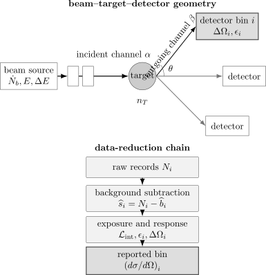
A scattering apparatus selects an incident channel $\alpha$, exposes a target with areal density $n_T$, and counts an outgoing channel $\beta$ in a detector bin with acceptance $\Delta\Omega_i$ and efficiency $\epsilon_i$. Background subtraction and exposure corrections are part of the map from records to $d\sigma_{\beta\leftarrow\alpha}/d\Omega$.

The beam and detector geometry also fixes the frame in which an angle is reported. For a light projectile scattering from a heavy fixed target, the laboratory and center-of-mass angles may nearly agree. For comparable masses they can differ substantially. A published angular distribution is incomplete unless its frame and angle convention are stated.

The target should usually be thin enough that a projectile undergoes at most one relevant collision. A thicker target raises the event rate, but it can also introduce energy loss, absorption, secondary interactions, and multiple scattering. More material is therefore not automatically more information.

Incident Flux and Luminosity

The incident flux density $j_b$ is the number of beam particles crossing unit area per unit time:

$$[j_b] = \frac{1}{\text{area}\,\text{time}}.$$

For a one-particle wavefunction, the corresponding quantum object is the probability current. For a beam, source intensity and particle number convert probability flux into particle flux. The local current and its normalization are developed in Probability Current.

Let $n_T(\mathbf x_\perp)$ be the target areal density, meaning the number of scattering centers per unit transverse area. The instantaneous luminosity is the beam–target overlap

$$\mathcal L(t) = \int_A d^2x_\perp\, j_b(\mathbf x_\perp,t) n_T(\mathbf x_\perp).$$

It has dimensions

$$[\mathcal L] = \frac{1}{\text{area}\,\text{time}}.$$

For a uniform beam fully covering a uniform thin target,

$$\mathcal L = \dot N_b\,n_T,$$

where $\dot N_b$ is the number of incident beam particles per unit time. The integrated luminosity, or total exposure, is

$$\mathcal L_{\mathrm{int}} = \int_{\text{run}}dt\,\mathcal L(t), \qquad [\mathcal L_{\mathrm{int}}] = \frac{1}{\text{area}}.$$

This language is not restricted to colliders. A radioactive source and foil, an electron gun and crystal, a molecular beam and gas jet, or a neutron beam and condensed-matter sample all require an exposure normalization, even when different communities use names such as fluence, monitor counts, incident charge, or beam current.

Differential Counting Rate

In an ideal detector resolving outgoing channel $\beta$ and solid angle $d\Omega$, the expected differential event rate is

$$\frac{dR_\beta}{d\Omega} = \mathcal L\, \frac{d\sigma_{\beta\leftarrow\alpha}}{d\Omega}.$$

A small detector of projected area $A_{\mathrm{det}}\cos\chi$ at distance $r$ subtends approximately

$$\Delta\Omega \simeq \frac{A_{\mathrm{det}}\cos\chi}{r^2},$$

where $\chi$ is the angle between the detector normal and the line from the target. If the cross section varies little across that bin, the expected signal count is

$$s_i \simeq \mathcal L_{\mathrm{int}}\, \epsilon_i\, \Delta\Omega_i \left( \frac{d\sigma_\beta}{d\Omega} \right)_i.$$

Here $\epsilon_i$ includes the probability that an event inside the accepted bin triggers, is reconstructed, and passes the analysis selection. Solving for the bin-averaged cross section gives

$$\left( \frac{d\sigma_\beta}{d\Omega} \right)_i \simeq \frac{s_i}{ \mathcal L_{\mathrm{int}} \epsilon_i \Delta\Omega_i }.$$

The narrow-bin formula is an approximation. A more faithful prediction folds the cross section through the apparatus response. Define

$$W_{i\beta}(t,E_f,\Omega) \equiv \mathcal L(t)\, \mathcal R_{i\beta}(E_f,\Omega),$$

where $\mathcal R_{i\beta}$ describes acceptance, efficiency, migration between bins, and event selection. Then

$$\begin{aligned} \mu_i&=s_i+b_i, \\ s_i ={}& \sum_\beta \int dt\,dE_f\,d\Omega \\ &\quad\times W_{i\beta}(t,E_f,\Omega) \frac{d^2\sigma_\beta}{dE_f\,d\Omega}. \end{aligned}$$

The expected count $\mu_i$ includes background $b_i$. This form assumes a fixed incident-energy setting; a beam with appreciable energy spread adds an integral over the calibrated incident-energy distribution. The equation expresses a central experimental fact: theory usually predicts a distribution in true kinematic variables, while the apparatus reports reconstructed bins.

Cross Section as Effective Area

For a uniform thin target with areal density $n_T$, the probability that one incident particle undergoes a process of total cross section $\sigma$ is

$$P_{\mathrm{int}} \simeq n_T\sigma, \qquad n_T\sigma\ll 1.$$

This gives the “effective area” interpretation. Each target center presents an interaction area $\sigma$, and the areal density determines how much of the incident ensemble is intercepted in the probabilistic sense.

If the interaction probability per unit depth is constant and scattered particles are simply removed from the incident beam, attenuation gives

$$P_{\mathrm{int}} = 1-e^{-n_T\sigma}.$$

The linear thin-target expression is its leading term. The exponential model is still idealized: energy loss, changing cross sections, secondary processes, and multiple scattering require transport theory or a detector simulation.

A cross section is not generally the literal geometric area of the target or constituent. Quantum interference, long-range forces, threshold enhancement, and resonances can make it much larger or smaller than a naive geometric estimate. The unit called a barn is

$$1\,\mathrm{b} = 10^{-28}\,\mathrm{m}^2.$$

Its convenience is historical; the physics lies in how $\sigma$ depends on energy, angle, spin, and channel.

Elastic and Inelastic Scattering

In elastic scattering, the asymptotic internal states of projectile and target are unchanged. Total energy and momentum are conserved, but kinetic energy can be redistributed between recoil partners in the laboratory frame. In the center-of-mass frame for one elastic channel,

$$\lvert\mathbf k_f\rvert = \lvert\mathbf k_i\rvert.$$

In inelastic scattering, some incident kinetic energy changes internal excitation, creates a different asymptotic channel, or produces additional particles when the theory permits it. A channel opens only when the incident energy exceeds its threshold. Different outgoing channel speeds then enter the flux normalization of the cross section.

For a probe that transfers momentum and energy,

$$\mathbf q = \mathbf p_i-\mathbf p_f, \qquad \hbar\omega = E_i-E_f.$$

An energy-resolving detector can therefore map a double-differential distribution such as

$$\frac{d^2\sigma}{d\Omega\,dE_f}.$$

For weak scattering from a many-body target, Structure Factors explains how this distribution factors into density or spin correlations, probe form factors, polarization projectors, kinematics, and resolution.

Elastic events lie on the kinematic elastic condition after recoil is included. Inelastic features identify target excitations or reaction channels. Whether the experiment is exclusive or inclusive depends on how completely the final state is specified:

• an exclusive measurement resolves a particular final channel and enough kinematics to identify it;
• an inclusive measurement sums over unobserved final states consistent with the recorded variables.

Calling a peak “elastic” solely because it is near zero measured energy transfer can be unsafe when the resolution is broader than low-energy excitations.

Acceptance, Resolution, and Background

Raw counts are not cross sections. At minimum, an analysis must consider:

• acceptance: the region of true phase space from which events can reach the detector;
• efficiency: the probability that an accepted event is triggered, recorded, reconstructed, and selected;
• resolution: the distribution of reconstructed values around the true values;
• background: counts from unrelated particles, detector noise, target supports, accidental coincidences, or competing channels;
• dead time and pileup: losses or distortions when events arrive too close together;
• normalization: uncertainty in beam exposure, target density, and live time;
• multiple scattering: angular and energy changes caused by more than one interaction in the target.

For observed counts $N_i$ and an independently estimated background $\widehat b_i$, a schematic signal estimate is

$$\widehat s_i = N_i-\widehat b_i.$$

If $N_i$ is a Poisson count with negligible background uncertainty, its statistical scale is $\sqrt{N_i}$. That does not include systematic uncertainty from efficiency, acceptance, calibration, background modeling, or luminosity. Reporting only counting statistics can therefore give a misleading impression of precision.

Finite resolution causes bin migration: an event generated in one true bin may be reconstructed in another. One can compare theory after forward-folding it through the response, or attempt to unfold the data. Forward-folding is often more stable because unfolding can amplify statistical fluctuations and introduce regularization dependence. Any unfolded result should state the response model and covariance matrix.

Worked Counting Example

Suppose a uniform beam has rate

$$\dot N_b = 2.0\times10^8\,\mathrm{s}^{-1}$$

and illuminates a thin target with

$$n_T = 5.0\times10^{22}\,\mathrm{m}^{-2}.$$

The luminosity is

$$\mathcal L = 1.0\times10^{31}\, \mathrm{m}^{-2}\mathrm{s}^{-1}.$$

For one angular bin, take

$$\begin{aligned} \frac{d\sigma}{d\Omega} &= 3.0\,\mathrm{b\,sr}^{-1}, \\ \Delta\Omega &= 2.0\times10^{-3}\,\mathrm{sr}, \\ \epsilon &= 0.60. \end{aligned}$$

The expected signal rate is

$$\begin{aligned} R_{\mathrm{sig}} &= \mathcal L\epsilon\Delta\Omega \frac{d\sigma}{d\Omega} \\ &= 3.6\,\mathrm{s}^{-1}. \end{aligned}$$

A $100\,\mathrm{s}$ run therefore gives an expected signal of $360$ events. The Poisson relative scale is approximately

$$\frac{\sqrt{360}}{360} \simeq 5.3\%.$$

If the luminosity has a $4\%$ calibration uncertainty and the efficiency has a $3\%$ uncertainty, those systematic contributions remain even if the run is made long enough to reduce the counting uncertainty.

The thin-target check for a $3\,\mathrm{b}$ process is

$$n_T\sigma = 1.5\times10^{-5},$$

so attenuation by that process is negligible. This check would have to include all important interaction channels, not only the angular bin being studied.

Historical Experiments

Two foundational experiments show how the same beam–target–detector logic can answer very different questions.

Rutherford scattering

Geiger and Marsden directed alpha particles from radioactive sources onto thin metal foils and counted scintillations at different angles. The rare large-angle events were decisive because a diffuse positive-charge model could not naturally produce them. Rutherford interpreted the angular distribution as evidence for a compact nuclear charge.

The historical apparatus, inference, and division of experimental labor are treated in Rutherford Scattering. The Coulomb amplitude and long-range asymptotics belong in Coulomb Scattering.

Davisson–Germer diffraction

Davisson and Germer used an electron gun, a nickel crystal, and a movable collector that measured scattered electron current versus angle and beam energy. Ordinary deflection was not the key result. Sharp angular maxima tied to the crystal spacing and electron momentum supplied the matter-wave evidence.

The apparatus and historical interpretation are treated in Davisson–Germer Experiment. This example also shows why a scattering experiment can measure phase information indirectly: amplitudes from different lattice planes interfere before the detector records an intensity.

These cases illustrate two durable uses of scattering:

Experimental pattern	Inference
rare events at large momentum transfer	localized structure at short distance
coherent angular maxima	wavelength, periodic order, and relative phase
resolved energy loss	internal excitations and available channels
energy-dependent enhancement	resonance or threshold structure

Scattering is therefore a form of controlled inference, not merely a way to make particles change direction.

From Data Back to Dynamics

The forward problem begins with a Hamiltonian and predicts a detector-level distribution after the apparatus response is included. The inverse problem begins with finite, noisy data and asks what interactions or target structure are compatible with them.

That inverse step is rarely unique. Cross sections often discard an overall amplitude phase, experiments cover finite angles and energies, and detector corrections can be model dependent. A fitted potential is therefore not automatically the uniquely reconstructed microscopic interaction. Inverse Scattering Preview develops these limitations.

A trustworthy comparison should state:

1. the incident and detected channels;
2. the laboratory or center-of-mass frame;
3. the exposure or luminosity normalization;
4. detector acceptance, efficiency, and resolution;
5. background treatment and uncertainty;
6. whether the theory was folded to detector level or the data were unfolded;
7. which parameters were inferred and which were externally constrained.

Common Mistakes

• Treating the number of detected events as an intrinsic property of the interaction without dividing by exposure, acceptance, and efficiency.
• Calling a cross section the physical size of the target. It is an interaction probability expressed as an effective area.
• Using detector area in place of solid angle without the distance and projection factor.
• Comparing a laboratory-angle distribution with a center-of-mass calculation without a kinematic transformation.
• Ignoring target thickness when multiple scattering or attenuation is appreciable.
• Assuming every event at the incident energy is elastic despite finite energy resolution.
• Subtracting a background estimate without propagating its uncertainty.
• Reading a potential directly from an angular histogram without addressing phase loss, finite coverage, and nonuniqueness.

Cross-Links

• How Quantum Matter Is Measured compares scattering counts with transport, spectroscopy, imaging, thermodynamic, and pump–probe records under one measurement-contract framework.
• Scattering Theory
• Probability Current
• Scattering Amplitude
• Differential and Total Cross Sections
• Coulomb Scattering
• Multichannel Scattering Preview
• Inverse Scattering Preview
• Structure Factors
• Rutherford Scattering
• Davisson–Germer Experiment

References

• J. R. Taylor, Scattering Theory: The Quantum Theory of Nonrelativistic Collisions, Wiley, 1972, Chapters 1–3.
• C. J. Joachain, Quantum Collision Theory, North-Holland, 1975, Chapters 1–3.
• R. G. Newton, Scattering Theory of Waves and Particles, 2nd ed., Springer, 1982.
• W. R. Leo, Techniques for Nuclear and Particle Physics Experiments, 2nd ed., Springer, 1994.
• G. Cowan, Statistical Data Analysis, Clarendon Press, 1998.
• H. Geiger and E. Marsden, “On a Diffuse Reflection of the α-Particles,” Proceedings of the Royal Society A 82, 495–500 (1909), DOI: 10.1098/rspa.1909.0054.
• E. Rutherford, “The Scattering of α and β Particles by Matter and the Structure of the Atom,” Philosophical Magazine 21, 669–688 (1911), DOI: 10.1080/14786440508637080.
• C. Davisson and L. H. Germer, “Diffraction of Electrons by a Crystal of Nickel,” Physical Review 30, 705–740 (1927), DOI: 10.1103/PhysRev.30.705.

Exercises

1. Luminosity dimensions

A beam of rate $\dot N_b$ uniformly illuminates a target with areal density $n_T$. Derive $\mathcal L=\dot N_b n_T$ from the overlap integral and verify its dimensions.

Solution

If the beam covers area $A$ uniformly, then $j_b=\dot N_b/A$. For constant $n_T$,

$$\mathcal L = \int_A d^2x_\perp\, \frac{\dot N_b}{A}n_T = \dot N_b n_T.$$

Because $[\dot N_b]=\mathrm{time}^{-1}$ and $[n_T]=\mathrm{area}^{-1}$,

$$[\mathcal L] = \mathrm{area}^{-1}\mathrm{time}^{-1}.$$

2. Thin-target limit

Starting from $P_{\mathrm{int}}=1-e^{-n_T\sigma}$, find the first two nonzero terms in the thin-target expansion. What dimensionless quantity controls the approximation?

Solution

Expanding the exponential gives

$$P_{\mathrm{int}} = n_T\sigma - \frac{(n_T\sigma)^2}{2} + \mathcal O\!\left((n_T\sigma)^3\right).$$

The dimensionless optical thickness $n_T\sigma$ controls the approximation. The linear expression is accurate when $n_T\sigma\ll1$ and when energy loss and secondary interactions can also be neglected.

3. One detector bin

A run has $\mathcal L_{\mathrm{int}}=4.0\times10^{32}\,\mathrm{m}^{-2}$, efficiency $\epsilon=0.50$, and solid angle $\Delta\Omega=5.0\times10^{-3}\,\mathrm{sr}$. After background subtraction, the bin contains $250$ signal events. Estimate $d\sigma/d\Omega$ in barns per steradian.

Solution

Using the narrow-bin formula,

$$\begin{aligned} \frac{d\sigma}{d\Omega} &\simeq \frac{250}{ (4.0\times10^{32}) (0.50) (5.0\times10^{-3}) } \\ &= 2.5\times10^{-28}\, \mathrm{m}^2\mathrm{sr}^{-1} \\ &= 2.5\,\mathrm{b\,sr}^{-1}. \end{aligned}$$

4. Elastic or inelastic?

A detector sees a narrow peak at the recoil-corrected elastic energy and a broader peak corresponding to a known target excitation. Classify the two features. Why can finite resolution complicate the classification?

Solution

The recoil-corrected peak belongs to the elastic channel because the target and projectile retain their internal states. The second peak is inelastic because energy is transferred into a target excitation. If the detector resolution is comparable to the excitation energy, the peaks overlap and events from the inelastic channel can migrate into the nominal elastic bin. Classification then requires a response model rather than a simple energy cut.

5. Acceptance bias

An angular distribution falls rapidly with $\theta$, but an analyst evaluates the theory only at the center of a wide detector bin. Explain the possible bias and give the correct comparison.

Solution

The value at the bin center need not equal the acceptance-weighted average when the cross section is curved or steep across the bin. The prediction should be integrated over the detector acceptance and folded with efficiency and angular resolution:

$$s_i = \int_{\text{bin}}d\Omega\, \mathcal L_{\mathrm{int}} \mathcal R_i(\Omega) \frac{d\sigma}{d\Omega}.$$

The folded count can then be compared directly with the observed bin.