Probability Current and Flux

Scattering observables are ratios of probability fluxes. The incoming beam supplies probability per unit area per unit time, while an outgoing spherical wave carries probability through distant surface elements. Their ratio has dimensions of area and becomes a cross section.

For a conservative one-particle Hamiltonian with real scalar potential, the current is

$$\begin{aligned} \mathbf j &= \frac{\hbar}{2\mu i} \left( \psi^*\nabla\psi - \psi\nabla\psi^* \right), \\ &= \frac{\hbar}{\mu} \operatorname{Im} \left( \psi^*\nabla\psi \right). \end{aligned}$$

where $\mu$ is the relevant mass or reduced mass. The general derivation and phase interpretation belong in Probability Current. This page is the canonical home for using that current in three-dimensional scattering, including the interference term that a quick derivation often hides.

Conservation Law

Probability density and current satisfy

$$\frac{\partial\rho}{\partial t} + \nabla\cdot\mathbf j = 0, \qquad \rho=\lvert\Psi\rvert^2.$$

For a stationary state

$$\Psi(\mathbf r,t) = e^{-iEt/\hbar} \psi(\mathbf r),$$

the density is time independent, so

$$\nabla\cdot\mathbf j=0$$

where the Hamiltonian is conservative and the wavefunction is regular. Integrating over a volume $\mathcal V$ gives

$$\oint_{\partial\mathcal V} \mathbf j\cdot d\mathbf S = 0.$$

The net current through any closed surface enclosing the interaction region therefore vanishes. This does not say that every part of the surface carries zero current. Incoming probability can cross one part of the surface and leave through another.

The integral conservation law is developed generally in Continuity Equation. Scattering turns it into a quantitative bookkeeping rule for channels and angles.

Incident Plane-Wave Flux

Let the incident beam point along $\hat{\mathbf z}$ and use the asymptotic plane wave

$$\phi_{\mathrm{in}}(\mathbf r) = A e^{ikz}.$$

Its current is

$$\mathbf j_{\mathrm{inc}} = \frac{\hbar k}{\mu} \lvert A\rvert^2 \hat{\mathbf z}.$$

Define the relative speed

$$v = \frac{\hbar k}{\mu}.$$

Then the incident flux magnitude is

$$j_{\mathrm{inc}} = v\lvert A\rvert^2.$$

The normalization amplitude $A$ may represent a box-normalized state, a delta-normalized basis state, or a beam intensity after an external conversion. The cross section will not depend on its overall magnitude because the outgoing wave carries the same factor.

A unit-flux plane wave uses an amplitude proportional to $v^{-1/2}$. This is particularly convenient when different channels have different velocities.

Current of an Outgoing Spherical Wave

For one elastic channel, write the leading scattered field as

$$\psi_{\mathrm{sc}}(\mathbf r) = A f(\hat{\mathbf r}) \frac{e^{ikr}}{r}.$$

Its radial derivative is

$$\partial_r\psi_{\mathrm{sc}} = \left( ik-\frac{1}{r} \right) \psi_{\mathrm{sc}}.$$

The radial current follows immediately:

$$\begin{aligned} j_r^{\mathrm{sc}} &= \frac{\hbar}{\mu} \operatorname{Im} \left( \psi_{\mathrm{sc}}^* \partial_r\psi_{\mathrm{sc}} \right) \\ &= \frac{\hbar k}{\mu} \lvert A\rvert^2 \frac{\lvert f(\hat{\mathbf r})\rvert^2}{r^2}. \end{aligned}$$

Thus the $1/r$ amplitude decay produces a $1/r^2$ flux density. Multiplication by the spherical area element

$$dS = r^2d\Omega$$

cancels the geometric dilution:

$$d\Phi_{\mathrm{sc}} = j_r^{\mathrm{sc}}r^2d\Omega = v\lvert A\rvert^2 \lvert f(\hat{\mathbf r})\rvert^2 d\Omega.$$

Angular variation also produces a tangential current of order $r^{-3}$:

$$\mathbf j_{\perp}^{\mathrm{sc}} = \frac{\hbar\lvert A\rvert^2}{\mu r^3} \operatorname{Im} \left[ f^*\nabla_\Omega f \right].$$

It is subleading compared with the radial $r^{-2}$ term and does not change the far-field differential cross section, but it is a useful reminder that an angle-dependent complex amplitude can carry transverse phase flow.

Differential Cross Section From Flux

The differential cross section is the scattered rate into $d\Omega$ divided by incident flux:

$$\frac{d\sigma}{d\Omega} = \lim_{r\to\infty} \frac{ r^2\, \hat{\mathbf r}\cdot \mathbf j_{\mathrm{sc}} }{ j_{\mathrm{inc}} }.$$

For the elastic convention above,

$$\frac{d\sigma}{d\Omega} = \lvert f(\hat{\mathbf r})\rvert^2.$$

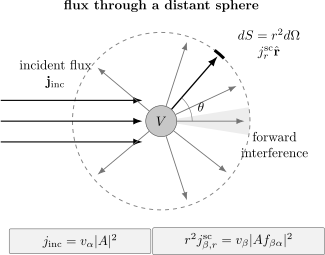
At large radius, the scattered current through $dS=r^2d\Omega$ remains finite because $j_r^{\mathrm{sc}}\propto r^{-2}$. Dividing that rate by the incident flux gives $d\sigma/d\Omega$. The total current also contains incident–scattered interference, concentrated into the forward limit after angular integration.

The definition uses the current assigned to the outgoing scattered component. It does not divide the total radial current by the incident current point by point. The total current also contains the incident plane wave and its interference with the scattered wave.

Differential and Total Cross Sections owns cross-section definitions, integration over final variables, and identical-particle conventions. The derivation here isolates the current structure behind those formulas.

Incident–Scattered Interference

For

$$\psi = \phi_{\mathrm{in}} + \psi_{\mathrm{sc}},$$

the current decomposes as

$$\mathbf j = \mathbf j_{\mathrm{inc}} + \mathbf j_{\mathrm{sc}} + \mathbf j_{\mathrm{int}},$$

where

$$\begin{aligned} \mathbf j_{\mathrm{int}} = \frac{\hbar}{\mu} \operatorname{Im} \Big( & \phi_{\mathrm{in}}^* \nabla\psi_{\mathrm{sc}} \\ &+ \psi_{\mathrm{sc}}^* \nabla\phi_{\mathrm{in}} \Big). \end{aligned}$$

Locally, $\mathbf j_{\mathrm{int}}$ is of order $1/r$, while the scattered current is of order $1/r^2$. This does not make the far-field cross section ill-defined. The interference term oscillates with phase

$$k(r-z) = kr(1-\cos\theta).$$

At fixed nonzero angle, those oscillations cancel under realistic angular averaging and in the large-$r$ distributional limit. Near $\theta=0$, however, the phase is stationary and the interference contribution survives.

This forward interference is essential. The incident plane wave by itself has zero net flux through a closed sphere:

$$\oint \mathbf j_{\mathrm{inc}} \cdot d\mathbf S = 0.$$

The scattered field carries positive outward flux, so conservation requires

$$\oint \left( \mathbf j_{\mathrm{sc}} + \mathbf j_{\mathrm{int}} \right) \cdot d\mathbf S = 0.$$

The negative integrated interference flux is the extinction of the incident beam. Evaluating it carefully gives the Optical Theorem. Dropping $\mathbf j_{\mathrm{int}}$ is harmless for deriving the differential cross section away from the forward cone, but it destroys the global conservation argument.

Surface Flux and Radial Wronskians

Current conservation becomes especially simple in a partial-wave channel. Let

$$\psi_{\ell m}(\mathbf r) = \frac{u_\ell(r)}{r} Y_{\ell m}(\hat{\mathbf r}),$$

with the spherical harmonic normalized to one. The integrated radial flux is

$$\Phi_\ell(r) = r^2 \int d\Omega\, j_r = \frac{\hbar}{\mu} \operatorname{Im} \left( u_\ell^* \frac{du_\ell}{dr} \right).$$

For a real potential and real energy, the radial equation implies

$$\frac{d\Phi_\ell}{dr} = 0.$$

Equivalently, the Wronskian of $u_\ell$ and $u_\ell^*$ is constant. If

$$u_\ell(r) \sim A_{\mathrm{out}}e^{ikr} + A_{\mathrm{in}}e^{-ikr},$$

then

$$\Phi_\ell = v \left( \lvert A_{\mathrm{out}}\rvert^2 - \lvert A_{\mathrm{in}}\rvert^2 \right).$$

Cross terms cancel in the radial current. For one conservative elastic channel, equal incoming and outgoing magnitudes imply

$$\lvert S_\ell\rvert=1.$$

This is the current-level origin of partial-wave unitarity. S-Matrix constructs the operator, Unitarity derives its channel constraints and bounds, and Phase Shifts expresses the elastic result as $S_\ell=e^{2i\delta_\ell}$.

Multichannel Flux

Suppose an incident channel $\alpha$ has speed $v_\alpha$, and an outgoing open channel $\beta$ has speed $v_\beta$. A common asymptotic convention is

$$\begin{aligned} \psi_\beta^{(\alpha)}(\mathbf r) \sim{}& \delta_{\beta\alpha} A_\alpha e^{i\mathbf k_\alpha\cdot\mathbf r} \\ &+ A_\alpha f_{\beta\alpha}(\hat{\mathbf r}) \frac{e^{ik_\beta r}}{r}. \end{aligned}$$

Orthogonal internal channel states do not interfere after the unresolved internal labels are traced or summed. The outgoing radial current in channel $\beta$ is

$$j_{\beta,r}^{\mathrm{sc}} = v_\beta \lvert A_\alpha\rvert^2 \frac{ \lvert f_{\beta\alpha}\rvert^2 }{r^2}.$$

Dividing by

$$j_{\alpha,\mathrm{inc}} = v_\alpha \lvert A_\alpha\rvert^2$$

gives

$$\frac{ d\sigma_{\beta\leftarrow\alpha} }{ d\Omega } = \frac{v_\beta}{v_\alpha} \lvert f_{\beta\alpha}\rvert^2.$$

The velocity ratio is not optional. Equal amplitude magnitudes can carry different fluxes when the channel momenta or reduced masses differ. A closed channel has imaginary $k_\beta$ and an evanescent asymptotic wave; it carries no flux to infinity even though it can modify open-channel scattering inside the interaction region.

With unit-flux channel functions, the factors $v_\alpha^{-1/2}$ and $v_\beta^{-1/2}$ are absorbed into state normalization. The resulting channel $S$-matrix is unitary when all open channels of a conservative theory are included.

Packets and Detector Probabilities

Stationary scattering states provide a steady flux rather than a normalized probability for one finite event. A normalizable packet restores the direct probability interpretation. If an outgoing packet crosses a distant detector surface $\Sigma_D$, then under clean one-way propagation its detection probability is represented by

$$P_D \simeq \int_{-\infty}^{\infty}dt \int_{\Sigma_D} \mathbf j(\mathbf r,t) \cdot d\mathbf S.$$

For a narrow packet, this time-integrated probability reproduces the stationary cross section after division by the integrated incident exposure. What Is a Scattering Experiment? develops the additional detector efficiency, acceptance, resolution, and background factors.

The approximation sign matters. Probability current is not a universal time-of-arrival probability density. Quantum backflow can make the current locally opposite to the momentum support, and a realistic detector is described by an interaction and a measurement model. In the far-field scattering regime with separated outward packets, the flux integral is the appropriate leading description.

Complex Potentials and Missing Channels

Let an effective optical potential be

$$V = V_R+iV_I.$$

The ordinary current then obeys

$$\frac{\partial\rho}{\partial t} + \nabla\cdot\mathbf j = \frac{2}{\hbar} V_I \rho.$$

If $V_I\lt0$, probability is removed from the explicitly modeled channel. Integrating over a volume gives

$$\oint_{\partial\mathcal V} \mathbf j\cdot d\mathbf S = \frac{2}{\hbar} \int_{\mathcal V} V_I \rho\,d^3r$$

for a stationary state. The right side is negative for absorption.

This does not mean fundamental probability conservation has failed. An optical potential represents channels that have been projected out. In the enlarged Hermitian theory, their outgoing flux restores unitarity. The reduced elastic $S$-matrix is subunitary because it does not contain those channels.

Scope and Caveats

• Vector potentials: with electromagnetic minimal coupling, use the gauge-covariant current

  $$\mathbf j = \frac{1}{\mu} \operatorname{Re} \left[ \psi^* \left( -i\hbar\nabla-q\mathbf A \right) \psi \right].$$

  Dropping the $\mathbf A$ term gives a gauge-dependent answer.

• Spinors: for a spin-independent Schrödinger kinetic term, replace $\psi^*\nabla\psi$ by the spinor inner product $\psi^\dagger\nabla\psi$. Spin-resolved cross sections then require explicit sums and averages.

• Nonlocal interactions: a nonlocal Hermitian potential need not admit the same simple local current equation with only the kinetic current. Integrated unitarity remains, but nonlocal transfer terms require care.

• Long-range forces: unscreened Coulomb scattering changes the asymptotic phase and produces a forward-divergent cross section. The simple separation into a plane wave and a short-range outgoing correction must be modified.

• Relativistic equations: Klein–Gordon and Dirac currents have different structures. The nonrelativistic current here should not be transplanted without rederivation.

Practical Checks

For an analytic or numerical scattering solution:

1. state the wavefunction and channel normalization;
2. compute incident and outgoing velocities;
3. verify that $r^2j_r^{\mathrm{sc}}$ approaches an $r$-independent angular distribution;
4. verify radial Wronskian or total flux conservation for a real potential;
5. include every open channel before testing unitarity;
6. inspect absorber, box-size, and matching-radius dependence in numerical work;
7. keep the forward interference term when testing the optical theorem.

These checks often catch missing velocity factors, wrong outgoing-wave signs, and imperfect numerical boundary conditions before they contaminate a reported cross section.

Common Mistakes

• Using $\lvert\psi\rvert^2$ instead of current to identify incident and outgoing rates.
• Dividing the total radial current by incident flux without separating the incident, scattered, and interference pieces.
• Discarding the interference term and then expecting global flux conservation or the optical theorem.
• Forgetting the factor $r^2$ when converting a radial current density into flux per solid angle.
• Omitting $v_\beta/v_\alpha$ in an inelastic or reaction channel.
• Calling an evanescent closed-channel tail an outgoing flux.
• Testing elastic-channel flux conservation when a complex optical potential or omitted open channels absorb probability.
• Using the zero-field current formula in the presence of a vector potential.
• Assuming a stationary density implies zero current.

Cross-Links

• Probability Current
• Continuity Equation
• Scattering States and Boundary Conditions
• Scattering Amplitude
• Differential and Total Cross Sections
• Optical Theorem
• Phase Shifts
• Multichannel Scattering Preview
• What Is a Scattering Experiment?
• Coulomb Scattering

References

• J. R. Taylor, Scattering Theory: The Quantum Theory of Nonrelativistic Collisions, Wiley, 1972, Chapters 3–5.
• R. G. Newton, Scattering Theory of Waves and Particles, 2nd ed., Springer, 1982.
• C. J. Joachain, Quantum Collision Theory, North-Holland, 1975.
• M. L. Goldberger and K. M. Watson, Collision Theory, Wiley, 1964.
• L. D. Landau and E. M. Lifshitz, Quantum Mechanics: Non-Relativistic Theory, 3rd ed., Pergamon, 1977.
• J. J. Sakurai and J. Napolitano, Modern Quantum Mechanics, 3rd ed., Cambridge University Press, 2020.
• H. Feshbach, “Unified Theory of Nuclear Reactions,” Annals of Physics 5, 357–390 (1958), DOI: 10.1016/0003-4916(58)90007-1.

Exercises

1. Plane-wave and spherical-wave currents

For $\phi=Ae^{ikz}$ and $\chi=Af(\hat{\mathbf r})e^{ikr}/r$, compute the incident current and the leading radial scattered current.

Solution

For the plane wave,

$$\nabla\phi = ik\hat{\mathbf z}\phi,$$

so

$$\mathbf j_{\mathrm{inc}} = \frac{\hbar k}{\mu} \lvert A\rvert^2 \hat{\mathbf z}.$$

For the scattered wave,

$$\partial_r\chi = \left( ik-\frac{1}{r} \right)\chi.$$

The real $-1/r$ term does not contribute to the imaginary part, giving

$$j_r^{\mathrm{sc}} = \frac{\hbar k}{\mu} \lvert A\rvert^2 \frac{\lvert f\rvert^2}{r^2}.$$

2. Recover the elastic cross section

Use the currents from Exercise 1 to derive $d\sigma/d\Omega=\lvert f\rvert^2$.

Solution

The scattered rate through $r^2d\Omega$ is

$$d\Phi_{\mathrm{sc}} = \frac{\hbar k}{\mu} \lvert A\rvert^2 \lvert f\rvert^2d\Omega.$$

Dividing by the incident flux

$$j_{\mathrm{inc}} = \frac{\hbar k}{\mu} \lvert A\rvert^2$$

gives

$$\frac{d\sigma}{d\Omega} = \lvert f\rvert^2.$$

Both the normalization amplitude and velocity cancel.

3. Multichannel velocity factor

An outgoing channel has speed $v_\beta=0.40v_\alpha$ and amplitude magnitude $\lvert f_{\beta\alpha}\rvert=3.0\,\mathrm{fm}$. Find the differential cross section in $\mathrm{fm}^2\mathrm{sr}^{-1}$.

Solution

The channel formula gives

$$\begin{aligned} \frac{d\sigma_{\beta\leftarrow\alpha}}{d\Omega} &= \frac{v_\beta}{v_\alpha} \lvert f_{\beta\alpha}\rvert^2 \\ &= 0.40(3.0\,\mathrm{fm})^2 \\ &= 3.6\,\mathrm{fm}^2\mathrm{sr}^{-1}. \end{aligned}$$

Using only $\lvert f\rvert^2$ would overestimate the outgoing flux by a factor of $2.5$.

4. Closed-surface balance

Why can the scattered current have positive outward flux through a large sphere even though the total flux through that sphere must vanish for a real one-channel potential?

Solution

The total current contains three pieces:

$$\mathbf j = \mathbf j_{\mathrm{inc}} + \mathbf j_{\mathrm{sc}} + \mathbf j_{\mathrm{int}}.$$

The incident plane wave has zero net flux through the closed sphere because as much enters one side as leaves the other. The scattered part has positive outward flux. The integrated interference term is negative in the forward region and exactly balances the scattered flux in a conservative one-channel problem. That balance is the current-space origin of the optical theorem.

5. Sign of an optical potential

For $V=V_R+iV_I$, determine which sign of $V_I$ represents absorption and explain how the missing flux is interpreted.

Solution

The continuity equation is

$$\frac{\partial\rho}{\partial t} + \nabla\cdot\mathbf j = \frac{2V_I}{\hbar}\rho.$$

Thus $V_I\lt0$ is a sink. In a stationary problem the outward surface flux is negative, meaning more probability enters the region than leaves through the explicitly retained channel. An optical potential summarizes channels that were projected out; in the full Hermitian theory, probability exits through those omitted channels rather than disappearing.