Phases of Matter in Many-Body QM

A phase of matter is a robust pattern of macroscopic organization shared by many microscopic states and Hamiltonians.

The word robust is essential. Small admissible changes to couplings, lattice details, or local basis choices should not erase the qualitative structure used to identify the phase. The word admissible is equally essential: the spatial dimension, locality class, symmetries, conservation laws, equilibrium setting, and spectral assumptions must be stated.

There is no single scalar test that classifies every many-body phase. A useful phase fingerprint can involve:

• thermodynamic potentials and their analyticity;
• symmetry and order parameters;
• long-distance correlation functions;
• spectral gaps and low-energy excitations;
• stiffnesses, susceptibilities, and quantized responses;
• topology, boundary structure, and defects;
• many-body entanglement.

Different phases require different subsets of this information. A ferromagnet is naturally described by broken symmetry and magnetic order. A Chern insulator can have no local symmetry-breaking order parameter but a quantized topological response. A Luttinger liquid is a stable gapless phase characterized by its low-energy theory and algebraic correlations rather than by a nonzero local order parameter.

Scope and Canonical Ownership

This page owns the general many-body concept of a phase:

• phase as stable qualitative behavior rather than one microscopic wavefunction;
• the relation among phase, state, regime, crossover, and transition;
• thermal and zero-temperature definitions;
• gapped adiabatic continuity and its assumptions;
• the special status of gapless phases;
• a multi-diagnostic phase fingerprint;
• robustness under allowed local perturbations;
• finite-size evidence standards;
• representative symmetry-breaking, superfluid, topological, and gapless examples.

Focused pages retain narrower ownership:

• Thermodynamic Limit owns bulk limiting sequences, boundary conditions, and noncommuting limits.
• Quantum Phase Transitions owns zero-temperature phase boundaries, gap closing, quantum critical scaling, and benchmark transitions.
• Finite-Temperature Phase Transitions owns thermal nonanalyticities, first-order and continuous transitions, critical temperatures, fluctuations, and finite-size rounding.
• Critical Exponents and Scaling owns the exponent dictionary, scaling relations, dynamic exponent, correction terms, and finite-size inference.
• Spontaneous Symmetry Breaking owns Hamiltonian versus state symmetry, source-selected infinite-volume phases, and finite-size spectral precursors.
• Symmetry-Protected Structure Preview owns protected degeneracies, boundary modes, and the hypotheses behind symmetry protection.
• Topological Invariants owns the mathematical definition and limitations of topological invariants.
• Entanglement Entropy in Many-Body Systems owns spatial scaling, area laws, critical logarithms, and topological corrections.

Universality owns the equivalence of critical points after microscopic metric factors are removed. Companion pages in this chapter own order parameters, long-range order, Goldstone modes, renormalization-group language, and Landau theory. Topological Order Preview owns the first integrated treatment of local indistinguishability, topology-dependent ground sectors, anyons, and long-range entanglement. Detailed material and model realizations belong to their dedicated Quantum Matter treatments.

Phase Is a Coarse-Grained Concept

A microscopic state is specified by a vector, density operator, or positive functional. A phase is an equivalence class or stable region containing many such states.

For a family of local Hamiltonians

$$H(\boldsymbol\lambda) = \sum_X h_X(\boldsymbol\lambda),$$

the parameters $\boldsymbol\lambda$ can include couplings, fields, pressure proxies, density, chemical potential, or interaction-to-hopping ratios. A phase occupies a region in this parameter space where a declared collection of bulk properties changes smoothly and remains qualitatively stable.

The phase concept deliberately forgets microscopic detail. Two samples can differ in lattice constants, short-range interactions, disorder realization, or quasiparticle velocities and still realize the same phase. Conversely, two Hamiltonians with identical microscopic symmetries can realize distinct phases if their long-distance structure cannot be connected under the allowed deformations.

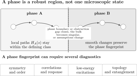
A phase is represented schematically as a connected region under admissible local deformations. Crossing to another phase requires an obstruction such as a bulk singularity, a closing of the relevant gap, or failure of a defining symmetry or constraint. No one diagnostic is universal; the phase fingerprint can combine order, correlations, response, excitations, topology, and entanglement.

State, Pure Phase, and Phase of Matter

The word phase is used at several levels.

Microscopic state

A finite-system density operator $\rho_L$ is one state. It can be changed continuously without defining a new phase every time an expectation value changes.

Infinite-volume equilibrium phase

In algebraic statistical mechanics, a pure thermodynamic phase is often represented by an extremal infinite-volume equilibrium state. A ferromagnet below its ordering temperature can have two symmetry-related extremal states with opposite magnetization. A convex mixture of them is also an equilibrium state but is not extremal.

Broad phase-of-matter label

In condensed-matter language, the symmetry-related positive- and negative-magnetization states are often called two broken-symmetry states within the same ferromagnetic phase of matter. Other authors call them distinct pure phases. Both usages occur.

The ambiguity is manageable if the object is named:

• state: one density operator or infinite-volume functional;
• pure thermodynamic phase: one extremal equilibrium state;
• phase of matter: a robust organizational class, often containing symmetry-related states.

Thermal Phases

For a finite region $\Lambda_L$ with Hamiltonian $H_L(\boldsymbol\lambda)$, define

$$Z_L(T,\boldsymbol\lambda) = \operatorname{Tr} \exp \left[ -\beta H_L(\boldsymbol\lambda) \right].$$

The finite-volume free-energy density is

$$f_L(T,\boldsymbol\lambda) = -\frac{k_{\mathrm B}T}{|\Lambda_L|} \ln Z_L(T,\boldsymbol\lambda).$$

For ordinary finite systems with finite matrix elements and $T\gt0$, $Z_L$ is positive and analytic in regular real coupling parameters. A sharp equilibrium transition therefore requires a bulk limit:

$$f(T,\boldsymbol\lambda) = \lim_{L\to\infty} f_L(T,\boldsymbol\lambda).$$

A conventional thermal phase is a connected region where the bulk thermodynamic functions and relevant local equilibrium properties are analytic, while phase boundaries are associated with nonanalytic behavior in the limit.

What analyticity captures

This language naturally captures:

• first-order coexistence surfaces;
• continuous ordering transitions;
• critical endpoints;
• singular response coefficients;
• latent heat and discontinuous densities;
• diverging correlation lengths.

What analyticity does not classify by itself

Knowing that $f$ is analytic inside a region does not tell the reader:

• which symmetry is broken;
• which quasiparticles exist;
• whether a response is quantized;
• whether boundary modes are protected;
• whether two zero-temperature gapped states are topologically distinct;
• how a stable gapless phase is organized.

Thermodynamics identifies sharp boundaries. The phase fingerprint supplies the physical content on either side.

Zero-Temperature Gapped Phases

At zero temperature, a powerful definition applies to local gapped Hamiltonians.

Consider a continuous path

$$H(s), \qquad 0\leq s\leq1,$$

with local or sufficiently rapidly decaying interactions. Suppose the relevant ground-state sector is separated from all higher excitations by a size-independent bulk gap:

$$\Delta_L(s) \geq \Delta_{\min} \gt 0$$

for sufficiently large $L$ and all $s$.

If the path also preserves the declared symmetries, dimensionality, locality class, and other defining constraints, then $H(0)$ and $H(1)$ are said to lie in the same gapped phase.

Ground-state manifolds

The phrase the gap remains open must specify the sector. A symmetry-breaking phase or intrinsically topological phase can have a ground-state manifold whose internal splitting vanishes with system size. The relevant gap is then the gap above that entire low-energy manifold, not necessarily

$$E_1-E_0$$

for one finite sample.

Let $P_L(s)$ project onto the chosen low-energy sector. A uniform spectral separation means that states outside the range of $P_L(s)$ remain at least $\Delta_{\min}$ higher in energy in the bulk limit.

Quasi-adiabatic continuation

Under locality and gap assumptions, quasi-adiabatic continuation constructs a quasi-local unitary $U(s)$ that transports the ground-state sector:

$$P(s) = U(s)P(0)U^\dagger(s).$$

The generator is built so that distant degrees of freedom are affected only through rapidly decaying tails. This makes the phase relation local in physical space rather than an arbitrary unitary equivalence of Hilbert spaces.

Every two normalized pure states in the same finite-dimensional Hilbert space are related by some global unitary. That statement is too weak to define a phase. The unitary must be local or quasi-local in a controlled sense.

Local-unitary viewpoint

For broad classes of gapped lattice states, the same-phase relation can also be expressed through finite-depth local circuits, possibly up to controlled approximation, stable ancillas, and symmetry constraints. Short-range entanglement can be rearranged locally; long-range entanglement cannot be removed by a finite-depth local circuit.

The exact equivalence among gapped paths, quasi-local evolutions, and circuit definitions depends on the setting. Gauge constraints, fermionic parity, crystalline structure, long-range interactions, and fracton geometry require additional care.

What Must Be Held Fixed?

A phase statement is incomplete until its admissible deformations are defined.

Spatial dimension

A one-dimensional chain and a two-dimensional layer are not normally compared as points in one phase space. Topological classifications and fluctuation effects depend strongly on dimension.

Locality class

For

$$H = \sum_X h_X,$$

the interaction norm and spatial decay matter. Stability theorems for short-range local Hamiltonians do not automatically apply to arbitrary all-to-all couplings.

Symmetry

Two states can be connected if symmetry breaking is allowed but remain distinct when a symmetry must be preserved. A symmetry-protected topological phase is defined only relative to its protecting symmetry and its action on the Hilbert space.

Conserved quantities and superselection

Particle-number conservation, fermion parity, gauge constraints, and charge sectors change the allowed paths. A superconducting mean-field Hamiltonian and an exactly number-conserving Hamiltonian require an explicit dictionary before their phases are compared.

Microscopic degrees of freedom

Adding a completely decoupled trivial ancilla should not usually create a new phase. This motivates stable equivalence. Adding a nontrivial topological layer, changing on-site symmetry representation, or changing filling can alter the classification.

Equilibrium or dynamical setting

An equilibrium phase, a metastable regime, a prethermal plateau, and a periodically driven phase are not interchangeable. This page concerns equilibrium thermal phases and ground-state phases unless stated otherwise.

Robustness Is Conditional

Let

$$H(\lambda) = H_0+\lambda V.$$

If $V$ is an allowed local perturbation and a defining bulk gap remains open for

$$|\lambda| \lt \lambda_c,$$

then the perturbed Hamiltonian stays in the same gapped phase.

This statement does not mean:

• every observable is unchanged;
• the gap has the same numerical value;
• quasiparticle masses and velocities are fixed;
• boundary spectra are independent of termination;
• disorder of arbitrary strength is harmless;
• a protecting symmetry may be broken freely.

Within one phase, nonuniversal quantities can vary substantially. Robustness means that the qualitative phase fingerprint and the stated obstruction do not disappear under allowed small changes.

Energy-scale criterion

For a gapped phase, a rough operational hierarchy is

$$\|V\|_{\mathrm{local}} \ll \Delta,$$

where $\|V\|_{\mathrm{local}}$ denotes a suitable local interaction scale rather than the extensive operator norm of the full perturbation. An extensive perturbation can have norm proportional to volume while still being weak per site.

The inequality is intuition, not a universal theorem. Rigorous stability depends on locality, interaction norms, ground-space structure, and additional hypotheses.

Gapless Phases

A gap-preserving definition cannot classify a phase whose bulk spectrum is gapless throughout a finite parameter region.

Examples include:

• a Fermi liquid with a stable Fermi surface;
• a one-dimensional Luttinger liquid;
• a superfluid with a Goldstone mode;
• a Coulomb phase with an emergent gauge mode;
• a critical phase with algebraic correlations.

For a gapless phase, stability is instead encoded by low-energy structure. Relevant descriptors can include:

• symmetry and conserved charges;
• the dimension and topology of a gapless manifold;
• central charge or other universal data;
• emergent gauge constraints;
• quasiparticle statistics;
• anomaly or Lieb–Schultz–Mattis-type obstructions;
• scaling exponents and operator content;
• the set of perturbations that are relevant, marginal, or irrelevant.

Same phase with varying exponents

In a Luttinger liquid, a continuous parameter $K$ can change correlation exponents while the system remains in the same broad gapless phase:

$$C_O(r) \sim \frac{\cos(qr)}{r^{\eta_O(K)}}.$$

The velocity and exponents vary, but the low-energy structure remains a compact bosonic mode with central charge $c=1$ over the stable region.

Boundaries inside gapless matter

A change in Fermi-surface topology, number of gapless modes, central charge, or allowed low-energy operator content can mark a phase transition even when both sides are gapless. The absence of a gap does not imply the absence of distinct phases.

There is no universal gapless classification comparable in simplicity to the gapped-path definition. The admissible low-energy theory must be stated.

The Phase Fingerprint

No single diagnostic should be promoted beyond its domain.

Thermodynamic structure

Useful quantities include:

$$f, \qquad s=-\frac{\partial f}{\partial T}, \qquad c_V = -T\frac{\partial^2 f}{\partial T^2},$$

and derivatives with respect to fields, pressure, or chemical potential.

Discontinuities or divergences can locate a boundary. Smooth values inside a phase characterize it but rarely classify it alone.

Symmetry and order

Let $G$ be a symmetry group of the Hamiltonian. A symmetry-breaking phase preserves only a subgroup

$$H\subset G.$$

An order parameter $M$ transforms nontrivially under $G$ and may satisfy

$$\lim_{h\to0^+} \lim_{L\to\infty} \langle M\rangle_{L,h} \ne 0.$$

The source $h$ selects one broken-symmetry state. Reversing the limits can return the symmetric finite-volume result.

Order parameters are powerful but not universal. Two phases can preserve the same symmetry and still differ topologically, in their excitation content, or in their pattern of entanglement.

Correlations

For a local observable $O$, define the connected equal-time correlation

$$C_O(\mathbf r) = \langle O(\mathbf r)O(\mathbf0) \rangle - \langle O(\mathbf r)\rangle \langle O(\mathbf0)\rangle.$$

Common long-distance patterns include:

$$C_O(r) \sim e^{-r/\xi}$$

for an ordinary short-range-correlated gapped phase,

$$C_O(r) \sim \frac{1}{r^\eta}$$

for a scale-invariant or stable algebraic phase, and

$$\lim_{r\to\infty} \langle O(\mathbf r)O(\mathbf0) \rangle \ne 0$$

for long-range order in the relevant channel.

These forms require qualifications for long-range interactions, disorder, finite temperature, conserved hydrodynamic modes, and operators with vanishing overlap on the slow sector.

Excitation spectrum

The spectral gap is

$$\Delta = \lim_{L\to\infty} \left[ E_{\mathrm{exc}}(L)-E_0(L) \right],$$

where the excitation sector must be declared.

Phase identity can also involve:

• Goldstone modes;
• magnons, phonons, or quasiparticles;
• particle and hole gaps;
• Fermi surfaces or nodal points;
• anyonic excitations and braiding;
• confined versus deconfined charges;
• protected boundary or defect modes.

Two phases can have the same ground-state symmetry but different elementary excitations.

Response

Response coefficients connect phase structure to probes. Examples include the compressibility

$$\kappa = \frac{\partial n}{\partial\mu},$$

the superfluid stiffness

$$\rho_s = \frac{1}{|\Lambda|} \left. \frac{\partial^2 F(\phi)}{\partial\phi^2} \right|_{\phi=0},$$

and a Hall conductance

$$\sigma_{xy} = C\frac{e^2}{h}$$

for an appropriate integer quantum Hall or Chern-insulator setting.

A response can vanish, remain finite, diverge, or become quantized. The relevant boundary conditions, order of limits, and units must be stated.

Topology

A topological invariant can distinguish phases that share local symmetry and bulk energy-gap properties. A change in an integer invariant cannot occur continuously while all assumptions defining it remain valid.

The safe inference is:

$$\begin{gathered} \text{different valid invariant} \\ \Longrightarrow \\ \text{a defining gap, symmetry,} \\ \text{or bundle hypothesis fails} \end{gathered}$$

along every interpolation.

The converse is not automatic. Equal values of one invariant do not prove that two interacting many-body states are in the same phase.

Entanglement

Entanglement can reveal organization invisible to local expectation values.

For a spatial region $A$,

$$S_A = -\operatorname{Tr} \left( \rho_A\ln\rho_A \right).$$

Broad one-dimensional gapped phases obey an area law, while critical one-dimensional phases often show logarithmic growth. Intrinsic topological order can contribute a universal subleading term in suitable geometries.

But:

• an area law alone does not classify a phase;
• two distinct gapped phases can have the same leading entropy scaling;
• finite-size entanglement spectra depend on the cut and symmetry sector;
• mixed-state and finite-temperature entanglement require different diagnostics.

Symmetry Is Central but Not Complete

Landau’s organizing principle classifies many phases by symmetry breaking.

Suppose

$$U(g)HU(g)^{-1} = H$$

for $g\in G$, while an ordered state is invariant only under $H_{\mathrm{unbroken}}\subset G$. Then the pattern

$$G \longrightarrow H_{\mathrm{unbroken}}$$

organizes order-parameter components, degeneracy, defects, and low-energy modes.

This framework explains magnets, crystals, superfluids, density waves, and many superconducting states. It does not exhaust quantum phases.

Same symmetry, distinct phase

Two charge-conserving two-dimensional insulators can preserve the same microscopic symmetries while having different Chern number. They cannot be connected while preserving the bulk gap and the assumptions behind that invariant.

Different symmetry does not specify everything

Knowing that spin rotation is broken does not by itself identify:

• whether the order is ferromagnetic or antiferromagnetic;
• the ordering wavevector;
• whether excitations are confined;
• whether another topological sector coexists;
• the transport and boundary response.

The full phase fingerprint remains necessary.

Topology and Long-Range Entanglement

Intrinsic topological order describes gapped many-body phases not reducible to local symmetry breaking. Depending on dimension and setting, signatures can include:

• topology-dependent ground-state degeneracy;
• anyonic quasiparticles;
• nontrivial braiding and fusion;
• long-range entanglement;
• topological entanglement entropy;
• robust boundary or defect structure.

Symmetry-protected topological phases are different. Their nontriviality requires specified symmetry protection. If that symmetry may be broken, a short-range-entangled SPT state can sometimes be connected to a trivial product-like state without closing the bulk gap.

This page uses these distinctions only to show why local order parameters are not universal classifiers. Topological Order Preview develops the diagnostic package; detailed classifications and realizations belong to Quantum Matter.

Low-Energy Excitations Are Part of the Phase

A phase is not merely its ground-state expectation values.

Ordered magnets

A ferromagnet and antiferromagnet can both break spin-rotation symmetry but have different ordering wavevectors and low-energy spin dynamics. Continuous symmetry breaking produces gapless collective modes under the appropriate assumptions.

Superfluids

A neutral superfluid has phase stiffness and a gapless sound mode. A charged superconductor couples the phase mode to electromagnetism, changing the low-energy spectrum through the Anderson–Higgs mechanism.

Insulators

Two insulators can both have vanishing zero-temperature compressibility and a bulk charge gap while differing in spin excitations, topology, polarization, or boundary states.

Fractionalized phases

The low-energy excitations can carry quantum numbers or statistics unavailable to microscopic particles. Fractionalization is then part of the emergent phase structure, not merely a small correction to a product state.

Example: Ising Ferromagnet and Paramagnet

Consider the transverse-field Ising family

$$H = -J \sum_j \sigma_j^z\sigma_{j+1}^z - h \sum_j \sigma_j^x.$$

It has a global spin-flip symmetry generated in a finite chain by

$$\mathcal P = \prod_j\sigma_j^x.$$

The two broad regimes are:

Diagnostic	Ferromagnetic regime	Paramagnetic regime
symmetry	broken in the thermodynamic pure states	preserved
order	long-range $\sigma^z$ correlations	no $\sigma^z$ long-range order
excitations	domain-wall-like sector	spin-flip-like sector
finite chain	symmetric parity eigenstates possible	symmetric ground state

A finite periodic chain can have

$$\langle\sigma_j^z\rangle=0$$

even when its correlation function and near-degenerate low-energy sector approach the ordered phase. One finite-size expectation value is therefore not a phase classifier.

The exact model, its finite-size spectrum, and its critical boundary are developed in Transverse-Field Ising Model and Quantum Phase Transitions.

Example: Mott Insulator and Superfluid

The Bose–Hubbard Hamiltonian is

$$\begin{aligned} H ={}& -t \sum_{\langle ij\rangle} \left( b_i^\dagger b_j + b_j^\dagger b_i \right) \\ &+ \frac{U}{2} \sum_i n_i(n_i-1) - \mu \sum_i n_i. \end{aligned}$$

At appropriate integer filling, two phases can be distinguished by several linked diagnostics.

Mott phase

In an idealized bulk Mott region:

$$\kappa=0$$

at zero temperature, particle and hole excitations are gapped, and the one-body density matrix has no off-diagonal long-range order.

Superfluid phase

The superfluid has nonzero stiffness,

$$\rho_s\gt0,$$

long-range or dimension-dependent quasi-long-range phase coherence, and a gapless collective phase mode in the thermodynamic limit.

The order parameter, compressibility, stiffness, gap, and correlation structure tell a consistent story. No one of them should be transplanted without its dimensional and finite-temperature qualifications.

Bose–Hubbard Model owns the model-specific phase diagram and conventions.

Example: Trivial and Chern Insulators

Two two-dimensional band insulators can share:

• charge conservation;
• a unique bulk ground state on a simple finite geometry;
• a nonzero bulk single-particle gap;
• exponentially decaying bulk correlations.

They can nevertheless differ by a Chern number

$$C = \frac{1}{2\pi} \int_{\mathrm{BZ}} d^2k\, \Omega_{xy}(\mathbf k),$$

when a noninteracting isolated-band description applies.

If

$$C_A\ne C_B,$$

there is no interpolation between the two band structures that keeps the relevant band gap open everywhere in the Brillouin zone while preserving the defining assumptions.

This is the cleanest reason symmetry labels alone do not classify all phases. The Berry-curvature and bundle construction belongs to Chern Numbers; interacting topological phases require broader many-body diagnostics.

Example: A Stable Gapless Liquid

The XXZ and spinless-fermion chains contain parameter regimes described at low energy by a Luttinger liquid.

Characteristic features include:

$$\Delta=0,$$

algebraic correlations,

$$C(r) \sim r^{-\eta},$$

linear low-energy dispersion,

$$E(k)-E_0 \sim \hbar v|k|,$$

and one compact gapless mode with

$$c=1.$$

The exponents and velocity vary continuously with interactions. This does not force a new phase at every value. A phase boundary appears when a relevant perturbation changes the stable low-energy structure, opens a gap, changes the number of modes, or produces a distinct ordered state.

See XXZ Spin Chain and Spinless-Fermion Chains for model-specific conventions and finite-size evidence.

Phase, Transition, and Crossover

These terms answer different questions.

Phase

A phase is a stable region with one declared qualitative organization.

Phase transition

A transition is the boundary or obstruction separating phases. It may be:

• first order;
• continuous;
• topological;
• a gap-opening transition;
• a transition between two gapless phases;
• driven by temperature, field, pressure, density, or a quantum coupling.

Crossover

A crossover is a smooth change in behavior with no sharp bulk singularity or protected obstruction in the stated parameter space.

For example, gas-like and liquid-like regimes above a liquid–gas critical endpoint can be connected without crossing a phase boundary. Their local structure changes substantially, but they belong to one analytic supercritical region.

Regime

A regime is a useful scale-dependent description. Terms such as quantum critical, hydrodynamic, collisionless, prethermal, or incoherent can describe behavior over a window without naming a distinct equilibrium phase.

Phase Diagrams Need Declared Axes

A phase diagram is a map only after its coordinates and ensemble are specified.

Common axes include:

$$T, \quad \mu, \quad h, \quad \frac{U}{t}, \quad \text{density}, \quad \text{pressure}.$$

Changing ensemble can change which variable is controlled and which thermodynamic potential is appropriate.

Lines, surfaces, and points

In a two-dimensional parameter plot:

• a phase boundary is commonly a line;
• a first-order line can end at a critical endpoint;
• several boundaries can meet at a multicritical point;
• a coexistence region can appear when an extensive density rather than its conjugate field is controlled;
• dashed lines often denote crossovers rather than transitions.

Graphical style is not physics. The caption must say which curves are singular boundaries, stability limits, or crossover estimates.

Finite Systems Do Not Contain Sharp Bulk Singularities

Every experiment and numerical calculation has finite size, finite resolution, finite time, and nonzero noise. The thermodynamic phase is inferred from systematic scaling.

Finite-temperature analyticity

For finite Hilbert space and $T\gt0$,

$$Z_L = \sum_n e^{-\beta E_n} \gt 0.$$

The real-axis free energy is analytic under ordinary parameter dependence. A sharp nonanalyticity appears only after a limiting sequence.

Finite zero-temperature smoothness

If a finite Hamiltonian depends analytically on $\lambda$ and has an isolated nondegenerate ground state with nonzero gap, its ground-state projector varies analytically near that point.

An avoided crossing can become increasingly sharp with size, but one narrow avoided crossing is not by itself a phase transition.

Useful finite-size evidence

Evidence can include:

• order-parameter scaling;
• Binder ratios;
• correlation-length ratios;
• gap scaling by symmetry sector;
• stiffness or compressibility scaling;
• entanglement scaling;
• topological response under twisted boundaries;
• collapse onto a controlled scaling form;
• stability under boundary-condition and truncation changes.

The correct evidence depends on the proposed phase.

Operational Phase Identification

A reliable classification proceeds in layers.

Step 1: Specify the system

State:

• microscopic degrees of freedom;
• dimensionality and geometry;
• interaction range;
• symmetries and conserved quantities;
• equilibrium ensemble;
• boundary conditions;
• thermodynamic sequence.

Step 2: State the candidate distinction

Examples:

• broken versus unbroken symmetry;
• gapped versus gapless;
• incompressible versus compressible;
• topologically trivial versus nontrivial;
• confined versus deconfined;
• one versus several gapless modes.

Step 3: Choose independent diagnostics

Use at least two conceptually distinct probes when feasible. For a proposed superfluid, for example:

• one-body correlations test coherence;
• stiffness tests response to a twist;
• the low-energy spectrum tests the phase mode;
• compressibility distinguishes some neighboring insulators.

Step 4: Perform scaling

Compare several sizes, shapes, and boundary conditions. Identify the scaling variable and leading corrections rather than reading a label from one finite plot.

Step 5: Stress-test robustness

Perturb the microscopic Hamiltonian within the allowed class. A feature that disappears under an arbitrarily small allowed perturbation may be accidental rather than phase-defining.

Step 6: State the obstruction

Explain why the candidate phases cannot be connected. The obstruction can be a bulk singularity, gap closing, symmetry change, topological invariant, long-range-entanglement distinction, or stable change in low-energy content.

Evidence Table

Claim	Minimum useful evidence	Important caveat
symmetry breaking	source or correlation scaling and order-of-limits statement	finite symmetric states can have zero one-point order
gapped phase	sector-resolved gap extrapolation and correlation behavior	the smallest finite-size splitting may lie inside the ground manifold
stable gapless phase	low-energy scaling over a parameter interval	one small gap at one size is not enough
topological phase	valid invariant or many-body response plus gap and symmetry hypotheses	edge states alone can depend on termination
superfluid	stiffness and coherence diagnostics	condensate fraction and superfluid density are not identical
first-order boundary	coexistence, hysteresis protocol, latent quantity, or volume scaling	metastability can mimic discontinuity
crossover	smooth bulk observables with no demonstrated obstruction	finite resolution cannot prove analyticity

Common Mistakes

• Calling every visually distinct parameter regime a phase.
• Defining a phase by one microscopic wavefunction.
• Saying “adiabatically connected” without requiring locality and a protected gap or low-energy structure.
• Using the extensive operator norm of a weak per-site perturbation as the only stability measure.
• Assuming a local order parameter exists for every phase.
• Treating equal symmetry as proof of equal phase.
• Treating different symmetry labels as a complete phase fingerprint.
• Calling every boundary state topologically protected.
• Quoting a topological invariant without its gap, symmetry, dimensional, and band or many-body assumptions.
• Using $E_1-E_0$ as the bulk excitation gap when $E_0$ and $E_1$ both belong to a collapsing ground-state manifold.
• Inferring spontaneous symmetry breaking from one arbitrarily chosen state in a small degenerate subspace.
• Inferring a phase transition from one finite-size level crossing.
• Confusing a finite-temperature crossover with a zero-temperature quantum phase transition.
• Calling a long-lived prethermal state an equilibrium phase without a dynamical definition.
• Assuming every gapless parameter point is a separate phase.
• Using entanglement entropy scaling alone to classify all gapped phases.
• Ignoring boundary conditions, aspect ratio, ensemble, or order of limits.

Exercises

Exercise 1: Product states and local equivalence

Consider spin-$1/2$ product states

$$|\Psi_0\rangle = |0\rangle^{\otimes L}$$

and

$$|\Psi_\theta\rangle = \left[ e^{-i\theta\sigma_y/2}|0\rangle \right]^{\otimes L}.$$

Show that a depth-one local unitary connects them. Construct a gapped on-site Hamiltonian path with these states as unique ground states.

Solution

Define

$$U_\theta = \bigotimes_{j=1}^{L} e^{-i\theta\sigma_j^y/2}.$$

All gates act on different sites, so they form a depth-one circuit. Directly,

$$|\Psi_\theta\rangle = U_\theta|\Psi_0\rangle.$$

Start from

$$H_0 = -\sum_j\sigma_j^z,$$

whose unique ground state is $|\Psi_0\rangle$. Let

$$U(s) = \bigotimes_j e^{-is\theta\sigma_j^y/2}$$

and define

$$H(s) = U(s)H_0U^\dagger(s).$$

Every $H(s)$ is a sum of on-site terms and has the same spectrum as $H_0$. The many-body gap is therefore constant:

$$\Delta(s)=2$$

in the units used here. The endpoint ground state is $|\Psi_\theta\rangle$. The states differ microscopically but lie in the same trivial gapped phase when no symmetry restriction forbids the rotation.

Exercise 2: Symmetry changes the answer

Suppose the path in Exercise 1 must preserve

$$U_z = \prod_j\sigma_j^z.$$

For generic $\theta$, does the rotation preserve this symmetry? What lesson follows for phase classification?

Solution

For one site,

$$\sigma_z e^{-i\theta\sigma_y/2} \sigma_z = e^{+i\theta\sigma_y/2},$$

which differs from the original rotation for generic $\theta$. Thus

$$[U_\theta,U_z]\ne0$$

in general.

The depth-one circuit proves equivalence only when arbitrary local basis rotations are allowed. If $U_z$ must be preserved, this particular path is inadmissible. Phase equivalence depends on the symmetry class and its on-site action, not only on the endpoint vectors.

Exercise 3: Why finite temperature is smooth at finite size

Let a finite Hamiltonian $H(\lambda)$ have eigenvalues $E_n(\lambda)$ that are analytic near $\lambda_0$. Show why

$$Z(\lambda) = \sum_n e^{-\beta E_n(\lambda)}$$

cannot vanish for real $\lambda$ and $\beta\gt0$. What does this imply for the finite-system free energy?

Solution

For real energies and positive $\beta$,

$$e^{-\beta E_n(\lambda)} \gt 0.$$

Therefore their finite sum satisfies

$$Z(\lambda)\gt0.$$

Each term is analytic, so $Z$ is analytic. Because it stays positive on the real axis, one can choose the ordinary real logarithm smoothly:

$$F(\lambda) = -k_{\mathrm B}T\ln Z(\lambda).$$

Thus the finite-system free energy has no real-axis thermodynamic singularity under these assumptions. Sharp phase transitions arise when a thermodynamic sequence converges nonuniformly and zeros or singular structures approach the physical axis in the limit.

Exercise 4: The correct gap in a broken-symmetry phase

A finite Ising-like chain has two lowest states with splitting

$$\delta_L \sim e^{-L/\ell},$$

while the next excitation lies an energy $\Delta_{\mathrm{bulk}}$ higher with

$$\Delta_{\mathrm{bulk}}\gt0$$

as $L\to\infty$. Which scale diagnoses the gap above the ordered ground-state manifold?

Solution

The two lowest states become the symmetry-related ground-state sector in the thermodynamic limit. Their internal splitting

$$\delta_L \longrightarrow 0$$

does not mean that the ordered phase lacks a bulk excitation gap.

Let $P_L$ project onto those two low-energy states. The relevant phase-protecting bulk gap is the separation from the range of $P_L$ to the rest of the spectrum:

$$\Delta_L^{\mathrm{out}} = E_2(L)-E_1(L) \longrightarrow \Delta_{\mathrm{bulk}}.$$

Using only $E_1-E_0$ would confuse the collapsing ground-state manifold with a gapless bulk mode.

Exercise 5: Same symmetry, different topology

Two two-dimensional noninteracting insulators preserve charge conservation and have Chern numbers

$$C_A=0, \qquad C_B=1.$$

Why can they not be connected through a path of isolated occupied bands that remains gapped everywhere in the Brillouin zone?

Solution

For an isolated occupied bundle, the Chern number is integer-valued and continuous under smooth deformations. A continuous integer-valued function is constant.

If a path connected $C_A=0$ to $C_B=1$ while the occupied subspace remained isolated and smooth for every $\mathbf k$, then $C$ would have to change continuously between two integers, which is impossible.

Therefore some defining hypothesis must fail. Typically the occupied and unoccupied bands touch at some momentum, closing the band gap. The two insulators preserve the same listed symmetry but belong to distinct gapped phases within this noninteracting class.

Exercise 6: Identify the Bose–Hubbard phase

A sequence of zero-temperature calculations gives

$$\kappa_L\longrightarrow0, \qquad \rho_{s,L}\longrightarrow0,$$

and a nonzero extrapolated particle-addition gap. Is this evidence for a superfluid or a Mott insulator at integer filling? What additional check is useful?

Solution

The vanishing compressibility, vanishing stiffness, and nonzero charge gap support a Mott-insulating phase rather than a superfluid.

A useful independent check is the one-body density matrix:

$$\langle b_i^\dagger b_j \rangle.$$

It should decay without off-diagonal long-range order in an ordinary Mott phase. One should also verify integer density, size convergence, and that the apparent gap is not a boundary or truncation artifact.

Exercise 7: Varying exponents inside one gapless phase

Suppose a one-dimensional model has, over an interval of coupling $g$,

$$C(r;g) \sim r^{-\eta(g)},$$

with continuously varying $\eta(g)$, one linearly dispersing mode, and central charge $c=1$. Must every value of $g$ define a distinct phase?

Solution

No. A gapless phase can contain continuously varying nonuniversal or marginally controlled parameters. In a Luttinger liquid, the Luttinger parameter changes correlation exponents while the stable low-energy structure remains one compact gapless bosonic mode with $c=1$.

A distinct phase requires a qualitative obstruction or change in the declared low-energy data, such as:

• opening a gap;
• changing the number of gapless modes;
• changing symmetry or an anomaly constraint;
• developing long-range order;
• changing Fermi or nodal topology;
• entering a different stable fixed-point family.

Continuous variation of $\eta$ alone does not force a phase boundary.

Exercise 8: Phase transition or crossover?

A finite system shows a rapidly changing density near $\lambda_\star$, but:

• the curve remains smooth;
• the peak susceptibility saturates with size;
• the correlation length remains much shorter than the system;
• no protected invariant or level-sector change is found.

What is the conservative interpretation?

Solution

The conservative interpretation is a crossover on the available evidence. A steep finite-size change can result from competing energy scales without converging to a bulk singularity.

To claim a transition, one would seek size-dependent evidence such as:

• susceptibility growth with a controlled scaling law;
• correlation length approaching the system size;
• latent-quantity or coexistence scaling;
• a sector-resolved gap closing;
• a topological invariant change under valid assumptions;
• a stable nonanalytic limit.

Failure to find such evidence does not mathematically prove analyticity at all scales, but it does not justify a phase-transition claim.

Cross-Links

• Symmetry-Protected Topological Phases — symmetry-restricted gapped paths, symmetric finite-depth circuits, projective edges, stacking, and anomaly inflow.

• Topological Order — long-range-entangled classification through anyon, modular, ground-space, entanglement, and response data.

• Thermodynamic Limit – bulk limits, boundary conditions, and orders of limits.

• Why Many-Body Physics Is Different – emergence, collective behavior, and the conceptual role of large systems.

• Quantum Phase Transitions – zero-temperature boundaries, critical scaling, and model benchmarks.

• Correlation Functions Overview – the general correlation dictionary.

• Connected Correlation Functions – subtraction of disconnected order and clustering diagnostics.

• Structure Factors – momentum-resolved density, spin, bond, and pair spectra.

• Susceptibilities – static and dynamic response channels.

• Spectral Functions – gaps, poles, continua, and evidence from line shapes.

• Spontaneous Symmetry Breaking – source selection, finite-size restoration, and broken-symmetry states.

• Symmetry-Protected Structure Preview – gap and symmetry protection.

• Topological Invariants – mathematical invariants and their domain of validity.

• Chern Numbers – Berry-curvature topology of isolated bands.

• Entanglement Entropy in Many-Body Systems – area laws, critical scaling, and topological terms.

• Lieb–Robinson Bound – locality bounds underlying quasi-local propagation and stability arguments.

• Transverse-Field Ising Model – symmetry-breaking benchmark.

• Bose–Hubbard Model – superfluid and Mott benchmark.

• XXZ Spin Chain – ordered, gapped, and Luttinger-liquid regimes.

• Spinless-Fermion Chains – fermionic gapless and charge-ordered regimes.

• Condensed-Matter Roadmap – a study path through phases and quantum matter.

References

1. P. W. Anderson, “More Is Different”, Science 177, 393–396 (1972).
2. L. D. Landau and E. M. Lifshitz, Statistical Physics, Part 1, 3rd ed., Butterworth–Heinemann (1980).
3. L. P. Kadanoff, “Scaling Laws for Ising Models Near $T_c$”, Physics Physique Fizika 2, 263–272 (1966).
4. N. Goldenfeld, Lectures on Phase Transitions and the Renormalization Group, CRC Press (2018).
5. S. Sachdev, Quantum Phase Transitions, 2nd ed., Cambridge University Press (2011).
6. C. N. Yang, “Concept of Off-Diagonal Long-Range Order and the Quantum Phases of Liquid He and of Superconductors”, Reviews of Modern Physics 34, 694–704 (1962).
7. M. B. Hastings and X.-G. Wen, “Quasi-Adiabatic Continuation of Quantum States”, Physical Review B 72, 045141 (2005).
8. X. Chen, Z.-C. Gu, and X.-G. Wen, “Local Unitary Transformation, Long-Range Quantum Entanglement, Wave Function Renormalization, and Topological Order”, Physical Review B 82, 155138 (2010).
9. X.-G. Wen, “Colloquium: Zoo of Quantum-Topological Phases of Matter”, Reviews of Modern Physics 89, 041004 (2017).
10. M. Z. Hasan and C. L. Kane, “Colloquium: Topological Insulators”, Reviews of Modern Physics 82, 3045–3067 (2010).
11. X.-L. Qi and S.-C. Zhang, “Topological Insulators and Superconductors”, Reviews of Modern Physics 83, 1057–1110 (2011).
12. M. P. A. Fisher, P. B. Weichman, G. Grinstein, and D. S. Fisher, “Boson Localization and the Superfluid–Insulator Transition”, Physical Review B 40, 546–570 (1989).
13. D. Ruelle, Statistical Mechanics: Rigorous Results, World Scientific (1999).
14. O. Bratteli and D. W. Robinson, Operator Algebras and Quantum Statistical Mechanics 2, 2nd ed., Springer (1997).