Precision Molecular Measurements

A precision molecular measurement uses resolved molecular states as a calibrated transducer between a microscopic interaction and a laboratory observable. Molecules are valuable because their electronic, vibrational, rotational, parity-doublet, and hyperfine structure can provide several resources at once:

• relativistically enhanced sensitivity to short-range electron interactions;
• large molecule-frame electric dipole moments that permit strong laboratory orientation;
• closely spaced opposite-parity levels that polarize in modest electric fields;
• internal reversals that change the signal sign without moving the apparatus;
• nuclear-spin and deformation sensitivity unavailable in a simple electronic transition; and
• long-lived states whose relative phase can be interrogated coherently.

An enhancement factor is not itself a measurement. A defensible result also requires a prepared state, a defined orientation convention, a protected comparison, calibrated molecular response coefficients, a systematic-error model, and a statistically identified mapping from the measured phase to microscopic parameters.

As of the review date, molecular experiments have set stringent null limits on symmetry-violating interactions, but no molecular experiment has established a nonzero electron electric dipole moment, nuclear Schiff moment, nuclear magnetic quadrupole moment, or parity-violating energy difference between enantiomers.

Canonical Scope

Tests of Fundamental Symmetries is the canonical home for the full EDM and parity-violation inference chain, reversal algebra, blinding, representative limits across molecular, atomic, neutron, and nuclear systems, and effective-operator interpretation. Cold Molecules owns molecular production, direct cooling, assembly, trapping, state preparation, and platform-level control. Rotations of Molecules derives rotor states, parity, Stark mixing, and rotational spectroscopy. Precision Spectroscopy owns line-centre estimation, correction budgets, and anomaly validation.

This page owns the molecule as sensor:

• how body-fixed structure becomes a laboratory-frame response;
• why the internal effective electric field is a matrix-element coefficient rather than an applied classical field;
• how molecular states probe electron-sector and nuclear-sector symmetry violation;
• what chiral spectroscopy would have to measure to isolate weak-interaction parity violation;
• how cold and trapped samples change the sensitivity and systematic budgets; and
• how molecular-structure theory enters calibration and global multi-operator fits.

The page emphasizes observable-first reporting. Particle-physics interpretations are important, but they come after the experiment has specified the measured channel and the molecular and nuclear conventions used to interpret it.

Knowledge Status

It is useful to separate four levels of claim.

• Established molecular physics: opposite-parity levels can be mixed by an electric field; heavy polar molecules can have large calculated relativistic response coefficients; and internal-state comparisons can reject common-mode fields.
• Established experimental result: several molecular platforms have measured frequency or phase channels consistent with zero symmetry-violating signal and have placed quantitative limits.
• Active development: trapped ions, laser-cooled beams, trapped polyatomics, nuclear-sensitive species, and enantiomer-resolved interferometers are extending coherence, count rate, internal comagnetometry, and operator complementarity.
• Theory-dependent interpretation: a system-level frequency bound becomes a bound on $d_e$, a semileptonic coupling, a nuclear moment, or a more fundamental operator only through declared electronic, molecular, nuclear, and sometimes hadronic calculations.

The distinction matters whenever a proposal, a demonstrated control technique, and a completed symmetry measurement are discussed together. A long coherence time or a large calculated enhancement can establish experimental capability without yet establishing a competitive limit.

The Molecular Inference Chain

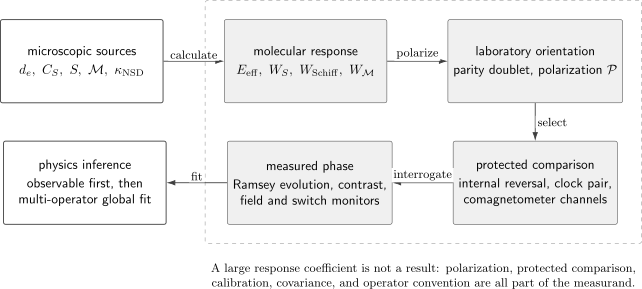
A molecular measurement is an inference chain, not a single enhancement factor. Molecular response coefficients such as $E_{\rm eff}$ become useful only after state orientation, protected comparison, phase calibration, and covariance-aware inference are specified.

Let $c_i$ denote microscopic or low-energy coefficients and let $a$ label a measured molecular channel. A useful linearized measurement model is

$$h\,\delta\nu_a = \sum_i \mathcal P_a W_{ai}c_i + \sum_j A_{aj}\eta_j + \epsilon_a.$$

Here:

• $\mathcal P_a$ is the laboratory orientation or another known angular factor;
• $W_{ai}$ is a molecular response coefficient in a declared convention;
• $\eta_j$ are nuisance quantities such as correlated magnetic fields, leakage-current proxies, geometric phases, or imperfect reversal magnitudes;
• $A_{aj}$ maps those nuisances into the measured channel; and
• $\epsilon_a$ contains statistical noise and any residual stochastic component represented by the covariance model.

For many channels this becomes

$$\mathbf y = K\mathbf c + A\boldsymbol\eta + \boldsymbol\epsilon, \qquad \operatorname{Cov} \left( \boldsymbol\epsilon \right) = \Sigma.$$

The rank and conditioning of $K$ determine which combinations of microscopic coefficients the data can identify. A single experiment with one response row generally constrains one linear combination, not every operator appearing in its effective Hamiltonian.

Why Molecules Can Amplify Small Effects

Several energy scales in one system

Electronic energies are typically much larger than vibrational energies, which are in turn much larger than rotational, hyperfine, and parity- doublet splittings. That hierarchy gives an experiment access to two features that would otherwise be difficult to combine:

1. heavy-atom electronic wavefunctions can have strong relativistic sensitivity near a nucleus; and
2. low-frequency rotational or parity structure can be mixed and read out with laboratory-scale fields.

The small denominator used for laboratory orientation and the large electronic matrix element used for microscopic sensitivity need not be the same physical energy scale.

Enhancement is operator-specific

There is no universal molecular enhancement factor. A candidate species has a response vector,

$$\mathbf W_a = \left( W_{a1}, W_{a2}, \ldots \right),$$

not a single scalar merit number. Increasing sensitivity to one operator may leave another unchanged, and two states of the same molecule may have different angular factors, lifetimes, magnetic moments, and systematic vulnerabilities.

For a parameter $c_i$, an operational definition is

$$W_{ai} = \left. \frac{\partial E_a}{\partial c_i} \right|_{\mathbf c=0}.$$

This derivative definition makes the convention visible. If $c_i$ is rescaled, $W_{ai}$ rescales inversely; the product $W_{ai}c_i$ is the physical energy.

Sensitivity is not precision

For an ideal Ramsey-like measurement of a coefficient $c$, a useful projection-noise scale is

$$\sigma_c \gtrsim \frac{\hbar} { C\,\tau\sqrt{N} \left| \partial\Delta E/\partial c \right| },$$

where $C$ is contrast, $\tau$ is coherent evolution time, and $N$ is the number of detected, statistically independent molecules. Real sensitivity also depends on duty cycle, dead time, technical noise, correlations, state-preparation and detection errors, and nuisance-parameter degeneracies.

A species with twice the response coefficient is not superior if it has one-tenth the coherent molecule number, much lower contrast, or a systematic channel that cannot be separated from the signal.

Internal Electric Fields

Body-fixed dipole versus laboratory orientation

A polar molecule can have a permanent body-fixed electric dipole

$$\mathbf D = D\,\hat{\mathbf n},$$

where $\hat{\mathbf n}$ is a directed molecular axis. In a field-free parity eigenstate, however,

$$\left\langle \hat{\mathbf n} \right\rangle = 0.$$

This is not a contradiction. The body-fixed charge distribution is polar, but a stationary parity eigenstate is an equal-amplitude superposition of opposite laboratory orientations.

An applied electric field mixes opposite-parity states and produces

$$\mathcal P \equiv \left\langle \hat{\mathbf n}\cdot\hat{\mathbf E} \right\rangle, \qquad -1\leq\mathcal P\leq1.$$

The distinction between $D$ and $\mathcal P$ is essential:

• $D$ controls the Stark coupling;
• the parity splitting controls how much field is needed;
• $\mathcal P$ states how strongly the selected level is oriented; and
• the microscopic response may have an additional electronic angular factor.

A two-state orientation model

Take opposite-parity states $|+\rangle$ and $|-\rangle$ separated by $\Delta_P$ and coupled by the dipole matrix element $D$. After removing a common energy, a convenient Hamiltonian is

$$H_{\rm orient} = \frac{\Delta_P}{2}\sigma_z - D\mathcal E\,\sigma_x,$$

where $\mathcal E$ is the signed laboratory electric field in the chosen axis convention. Its eigenenergies are

$$E_\pm = \pm \frac12 \sqrt{ \Delta_P^2 + 4D^2\mathcal E^2 }.$$

For the lower adiabatic state, the magnitude of the orientation follows from the Hellmann–Feynman theorem:

$$\mathcal P = \frac{1}{D} \left| \frac{\partial E_-}{\partial\mathcal E} \right| = \frac{ 2D|\mathcal E| }{ \sqrt{ \Delta_P^2 + 4D^2\mathcal E^2 } }.$$

Thus

$$\mathcal P \simeq \frac{2D|\mathcal E|}{\Delta_P} \quad \text{for } D|\mathcal E|\ll\Delta_P,$$

while $\mathcal P\rightarrow1$ for strong mixing. Closely spaced parity doublets can therefore reach nearly complete polarization at fields much smaller than those needed to mix ordinary rotational levels.

The two-state model is an orientation model, not a complete molecular Hamiltonian. Hyperfine interactions, tensor Stark shifts, nearby rotational states, avoided crossings, and field-dependent magnetic moments must be included when they are comparable to the target accuracy.

What the effective electric field means

In an electron-EDM experiment, $E_{\rm eff}$ is defined from a relativistic molecular matrix element. Schematically,

$$\Delta E_{d_e} = -d_e E_{\rm eff} \Omega\mathcal P,$$

where $\Omega$ is the signed projection of electronic angular momentum on the molecular axis in one common convention.

$E_{\rm eff}$ is not:

• the applied electrode field;
• the electrostatic field at a classical electron position;
• a quantity that can be inserted into an unrelated nonrelativistic Stark Hamiltonian; or
• directly measured by polarizing the molecule.

It is a response coefficient obtained from a relativistic electronic- structure calculation. The very large values quoted for heavy polar molecules summarize how a specified $P,T$-odd electron operator shifts a particular molecular state.

Why heavy polar species are useful

The electron-EDM interaction strongly samples relativistic electronic wavefunctions near a heavy nucleus. Useful candidates often combine:

• a heavy atom that supplies large relativistic matrix elements;
• an electronic state with unpaired spin density near that atom;
• a polar bond that defines a body-fixed axis;
• low-lying opposite-parity structure for laboratory orientation; and
• a metastable or ground-state manifold with practical preparation and readout.

Simple powers of nuclear charge are valuable scaling intuition, but they are not a substitute for molecular calculation. Chemical bonding, configuration mixing, core polarization, electron correlation, finite nuclear size, and state assignment all affect the response.

Theory is part of the calibration

A credible response coefficient should come with:

1. the effective operator and normalization;
2. the electronic state and phase convention;
3. basis-set and correlation convergence tests;
4. treatment of relativistic and finite-nucleus effects;
5. comparisons among independent methods where possible;
6. benchmarks against ordinary observables sensitive to similar wavefunction regions; and
7. an uncertainty or defensible spread, not only a preferred number.

Dipole moments, hyperfine constants, level intervals, and spectroscopic constants cannot prove a symmetry-violating matrix element, but agreement with them can test important parts of the wavefunction. A calculation that does not reproduce relevant ordinary observables should not be treated as an exact conversion factor.

Electron EDM Searches

What the experiment measures

For a paramagnetic molecular state, a schematic $P,T$-odd energy is

$$\Delta E_{P,T} = -\Omega\mathcal P \left( d_e E_{\rm eff} + C_S W_S + \cdots \right).$$

Here $C_S$ denotes a scalar electron–nucleon coupling in one common normalization and $W_S$ is its molecular response. Other operators can be added when they are relevant at the claimed precision.

Suppose the reported channel is the energy difference between a pair of spin-projection states whose $d_e$ shifts have opposite sign. Declaring $E_{\rm eff}>0$ as a magnitude, one convenient pair convention is

$$\Delta E_{\rm pair} = 2\mathcal P d_e E_{\rm eff}.$$

The corresponding Ramsey phase is

$$\phi_{d_e} = \frac{ \Delta E_{\rm pair}\tau }{\hbar} = \frac{ 2\mathcal P d_e E_{\rm eff}\tau }{\hbar}.$$

Another paper may absorb the factor of two, $\Omega$, or an orientation sign into its definition of frequency. Numerical results should be translated through the published Hamiltonian, not compared by symbol matching.

Ramsey readout and reversals

A typical sequence is:

1. prepare a coherent superposition of magnetic or hyperfine sublevels;
2. let the relative phase evolve in electric and magnetic fields;
3. close the interferometer with a second pulse or state rotation;
4. detect a spin population or asymmetry; and
5. repeat under a balanced set of field and internal-state reversals.

With binary switches $s_q=\pm1$, any measured frequency can be expanded as

$$f(\mathbf s) = \sum_{S} f^S \prod_{q\in S}s_q.$$

The nominal EDM channel is the coefficient with the signal’s expected switch parity. That projection rejects many ordinary shifts, but it does not prove their absence. An ordinary effect that is correlated with the same switch product leaks into the same coefficient.

Important monitors include:

• actual electric- and magnetic-field magnitudes in every switch state;
• leakage current and charging transients;
• state-dependent fluorescence or ion loss;
• preparation and readout asymmetries;
• field gradients and motional correlations;
• pulse phase, amplitude, and detuning;
• trap or beam trajectory changes; and
• correlations between all of these and the target switch channel.

Internal reversals

Some molecular manifolds contain nearby states with opposite molecular orientation but nearly the same magnetic environment. Comparing them reverses the $P,T$-odd response while largely preserving ordinary Zeeman shifts. This internal comagnetometer can be more powerful than comparing spatially separated samples.

It is not exact. The partner states may have different:

• magnetic $g$ factors;
• tensor Stark shifts;
• transition strengths and line pulling;
• geometric phases;
• trap potentials or trajectories; and
• preparation and detection efficiencies.

The residual differences belong in the measurement model and should be exaggerated experimentally where possible.

Current experimental status

The strongest published single-source electron-EDM limit reviewed on 2026-07-26 comes from trapped HfF$^+$ molecular ions:

$$d_e = \left( -1.3 \pm2.0_{\rm stat} \pm0.6_{\rm syst} \right) \times10^{-30}\ e\,{\rm cm},$$

with

$$|d_e| < 4.1\times10^{-30}\ e\,{\rm cm} \qquad \text{at 90\% confidence}.$$

The conversion assumes that other contributing sources, notably $C_S$ in the experiment’s chosen operator basis, vanish. The trapped-ion platform used coherence times up to about $3\ {\rm s}$ and a calculated $E_{\rm eff}$ of about $23\ {\rm GV\,cm^{-1}}$.

The ACME ThO beam result provides an important independent architecture:

$$|d_e| < 1.1\times10^{-29}\ e\,{\rm cm} \qquad \text{at 90\% confidence},$$

with a calculated effective field of roughly $78\ {\rm GV\,cm^{-1}}$. Its high-flux beam, metastable electronic state, and internal comagnetometer have a very different systematic ledger from the trapped-ion experiment.

Platform	Precision resource	Internal control	Principal cost
ThO beam	large $E_{\rm eff}$ and high detected flux	opposite-orientation doublet	millisecond-scale transit time
trapped HfF$^+$	second-scale coherent evolution	rotating-field orientation and paired states	trap fields, ion motion, and lower count rate
cold YbF beam	low velocity and controlled spin interferometry	field and state reversals	source flux and end-to-end detection
trapped CaOH or YbOH	long interaction and parity-doublet structure	internal comagnetometry and engineered clock pairs	trap shifts, state loss, collisions, and complex manifolds

Recent milestones should be described according to what they establish:

• coherent control of trapped CaOH demonstrated an electron-EDM-sensitive polyatomic measurement architecture, but the light Ca centre does not provide a competitive electron-EDM enhancement;
• engineered YbOH clock transitions demonstrated strong suppression of electric and magnetic sensitivity while retaining an electron-EDM response, but did not report a new EDM limit; and
• ultracold YbF beam spin interferometry demonstrated the control sequence needed for a future high-sensitivity measurement, rather than a new symmetry-violation signal.

This distinction prevents projected reach from being presented as a measured exclusion.

Single-source limits and global fits

A measured molecular channel can constrain

$$y_a = K_{ae}d_e + K_{aS}C_S + \cdots.$$

Setting $C_S=0$ yields a valid conditional limit on $d_e$, provided the assumption is stated. It does not make the experiment intrinsically insensitive to $C_S$.

With several systems,

$$\begin{pmatrix} y_1\\ y_2\\ \vdots \end{pmatrix} = \begin{pmatrix} K_{1e} & K_{1S} & \cdots\\ K_{2e} & K_{2S} & \cdots\\ \vdots & \vdots & \ddots \end{pmatrix} \begin{pmatrix} d_e\\ C_S\\ \vdots \end{pmatrix}.$$

Complementarity comes from nonparallel response rows, not simply from adding more measurements of nearly the same species class. Experimental covariance and correlated theory uncertainties should be carried into the fit.

Nuclear Symmetry Tests

Why molecules can probe nuclei

Electrons in a polar molecule repeatedly sample the heavy nucleus and translate short-range nuclear interactions into spectroscopic shifts. Molecular orientation then provides a controllable laboratory axis relative to nuclear spin.

The main candidate observables include:

• a nuclear Schiff moment $\mathcal S$;
• a nuclear magnetic quadrupole moment $\mathcal M$;
• nuclear-spin-dependent parity violation through $\kappa_{\rm NSD}$; and
• isotope-dependent weak and hyperfine effects used to constrain nuclear structure.

These observables are distinct. A species optimized for one is not automatically optimal for the others.

Schiff screening and the Schiff moment

For nonrelativistic point charges interacting electrostatically in a neutral bound system, a pointlike nuclear EDM is screened at leading order. Schiff’s theorem does not say that a real atom or molecule is insensitive to all nuclear $P,T$ violation. Finite nuclear size, relativistic effects, magnetic interactions, and $P,T$-odd nuclear forces evade its assumptions.

The residual finite-size source is often organized as a nuclear Schiff moment $\boldsymbol{\mathcal S}$. A molecular effective Hamiltonian may be written schematically as

$$H_{\mathcal S} = W_{\mathcal S} \mathcal S \frac{ \mathbf I\cdot\hat{\mathbf n} }{I},$$

where $W_{\mathcal S}$ is an electronic-structure coefficient and the definition of $\mathcal S$ depends on the nuclear convention.

The inference chain is layered:

$$\text{frequency} \longrightarrow \mathcal S \longrightarrow \text{nuclear }P,T\text{-odd couplings} \longrightarrow \text{hadronic or fundamental operators}.$$

Each arrow has its own calculation and uncertainty. A molecular frequency limit should not be translated through all layers with an unexplained single factor.

Octupole-deformed nuclei

Some heavy nuclei have reflection-asymmetric, octupole-correlated structure and low-lying opposite-parity nuclear states. In a schematic two-state picture,

$$\mathcal S_{\rm lab} \simeq 2\,\operatorname{Re} \left[ \frac{ \langle +|\widehat{\mathcal S}|-\rangle \langle -|V_{P,T}|+\rangle }{ E_+-E_- } \right].$$

A small nuclear parity splitting can enhance the laboratory Schiff moment. The enhancement remains nuclear-model dependent: deformation, pairing, configuration mixing, and the $P,T$-odd nuclear interaction all enter. RaF and AcF are attractive partly because radium and actinium isotopes can combine heavy-atom electronic response with unusual nuclear structure.

Laser spectroscopy of RaF has directly tested short-range electron–nucleus sensitivity through the distribution of nuclear magnetization, and gas-phase AcF spectroscopy has established key spectroscopic and theoretical information for proposed $CP$-violation searches. Neither result is a detection of a Schiff moment.

Nuclear magnetic quadrupole moments

A $P,T$-odd nuclear magnetic quadrupole moment couples nuclear spin to the electronic and molecular axis through a tensor interaction. It can be represented schematically by

$$H_{\mathcal M} = W_{\mathcal M} \mathcal M \Xi_{\mathcal M},$$

where $\Xi_{\mathcal M}$ is a dimensionless angular operator determined by the electronic state, total angular momentum, and hyperfine basis.

Open-shell molecules can be especially useful because electronic angular momentum supplies the magnetic-field gradient needed to couple to $\mathcal M$. Deformed nuclei may provide collective enhancement. A reported limit must specify the angular convention used for both $W_{\mathcal M}$ and $\mathcal M$.

Nuclear-spin-dependent parity violation

One common low-energy form for nuclear-spin-dependent parity violation is

$$H_{\rm NSD} = \frac{G_F}{\sqrt2} \kappa_{\rm NSD} \rho_N(\mathbf r) \boldsymbol{\alpha}\cdot \frac{\mathbf I}{I},$$

where $G_F$ is the Fermi constant, $\rho_N$ is a normalized nuclear density, and $\boldsymbol{\alpha}$ is a Dirac matrix vector for the electron. The dimensionless coefficient $\kappa_{\rm NSD}$ can receive contributions from:

• the nuclear anapole moment;
• electron–nucleon neutral-current interactions; and
• combined nuclear-spin-independent weak and hyperfine mixing.

Near-degenerate opposite-parity molecular levels can enhance the mixing produced by $H_{\rm NSD}$. Experiments seek an interference term between a weak, parity-odd amplitude and a controlled parity-even amplitude. The signal changes sign under selected field, state, or isotope reversals.

BaF experiments have demonstrated the required near-degeneracy control and sub-hertz sensitivity to a nuclear-spin-dependent parity-violating matrix element. These are method and sensitivity demonstrations, not an observed molecular anapole signal.

Representative nuclear-sensitive programmes

System or programme	Primary molecular resource	Target	Status at review date
BaF	opposite-parity rotational and hyperfine levels	nuclear-spin-dependent parity violation	method and systematic-control demonstrations; no detected NSD-PV signal
TlF and CeNTREX	heavy diamagnetic molecule and long molecular beam	$^{205}$Tl Schiff moment	experiment under development; projected sensitivity is not a result
RaF	heavy nucleus with octupole correlations and laser-addressable molecule	Schiff and related nuclear moments	spectroscopy and nuclear-magnetization sensitivity demonstrated; no $CP$-odd signal
AcF	heavy, potentially strongly enhanced nuclear system	Schiff moment and hadronic $CP$ violation	first gas-phase spectroscopy and theory benchmarks; sensitivity remains prospective

The most trustworthy way to report these programmes is to name the measured quantity first: a line frequency, an interference amplitude, a hyperfine anomaly, a coherence time, or a null switch coefficient. The target nuclear parameter belongs in the next layer of the statement.

Chiral Molecules and Parity Violation

Chirality is not itself weak-interaction parity violation

A chiral molecule has two enantiomeric structures, conventionally denoted $|L\rangle$ and $|R\rangle$, that are related by parity:

$$\mathsf P|L\rangle = |R\rangle, \qquad \mathsf P|R\rangle = |L\rangle.$$

Electromagnetic interactions that conserve parity give the two enantiomers equal intrinsic energies. The electroweak interaction can produce a tiny parity-violating energy difference.

Enantiomer-specific microwave detection, three-wave mixing, optical rotation, circular dichroism, and enantiomer-selective state transfer can distinguish handedness. Those techniques do not by themselves measure the weak parity-violating energy difference. They are preparation and readout tools for a possible precision comparison.

Likewise, chemistry-dependent chiral discrimination and spin-selective transport effects should not be relabelled as a molecular weak-interaction measurement without a demonstrated connection to the parity-violating Hamiltonian.

Localized-state model

Let

$$\epsilon_{\rm PV} \equiv \frac{E_R-E_L}{2}$$

and let $\Delta_{\rm tun}$ be the parity-conserving tunnelling splitting between the two localized structures. A minimal Hamiltonian is

$$H_{\rm chiral} = \begin{pmatrix} E_0+\epsilon_{\rm PV} & -\Delta_{\rm tun}/2\\ -\Delta_{\rm tun}/2 & E_0-\epsilon_{\rm PV} \end{pmatrix}.$$

Its eigenvalue splitting is

$$\Delta E = \sqrt{ \Delta_{\rm tun}^2 + 4\epsilon_{\rm PV}^2 }.$$

Two lessons follow.

First, if $\Delta_{\rm tun}$ is much larger than $|\epsilon_{\rm PV}|$, the parity-eigenstate splitting changes only quadratically in $\epsilon_{\rm PV}$. A naive search for a linear shift of that splitting is poorly conditioned.

Second, if the experiment prepares states localized in handedness or compares enantiomer-resolved transitions, a linear differential observable can be formed. For a transition between lower and upper internal levels,

$$\delta\nu_{\rm PV} = \nu_R-\nu_L = \frac{ 2\left( \epsilon_{\rm PV}^{(e)} - \epsilon_{\rm PV}^{(g)} \right) }{h}.$$

The relevant quantity is the difference of parity-violating energies between the two spectroscopic states, not the absolute parity-violating energy of one structure.

What a credible search needs

A molecular chiral-parity experiment needs:

1. enantiopure or enantiomer-resolved preparation;
2. a transition with a calculated differential weak response;
3. frequency comparison in the same field and time reference;
4. controlled interchange of handedness;
5. suppression or calibration of ordinary enantiomer-dependent chemical, collisional, Stark, Zeeman, and light shifts;
6. a model of tunnelling and conformer exchange;
7. line-shape and unresolved-mixture tests; and
8. independent verification of handedness and state populations.

Simultaneous Ramsey comparison of both enantiomers is attractive because common oscillator noise can cancel. It also creates new requirements: the two samples must experience demonstrably equivalent fields, collisions, ac Stark shifts, and detection response.

No unambiguous parity-violating enantiomer energy difference had been observed by the review date. Existing enantiomer-specific microwave control is enabling technology, not evidence for a weak-interaction splitting.

Cold-Molecule Advantages

What cooling can improve

Slower or trapped molecules can provide:

• longer coherent interaction time $\tau$;
• narrower transit-time and Doppler distributions;
• repeated interrogation or state-selective imaging;
• resolved motional and internal states;
• lower motional magnetic fields;
• tunable collisions and controlled density;
• confinement in shielded, mapped regions; and
• access to polyatomic parity doublets and internal comagnetometers.

These gains are especially valuable when a signal phase grows linearly with time:

$$\phi_c = \frac{ \Delta E(c)\tau }{\hbar}.$$

What cooling can cost

Cooling does not guarantee better sensitivity. The statistical information per unit averaging time scales schematically as

$$\mathcal I_c \propto \frac{ N_{\rm cyc}C^2\tau^2 }{ T_{\rm cyc} } \left( \frac{\partial\Delta E}{\partial c} \right)^2,$$

where $N_{\rm cyc}$ is the detected count per cycle and $T_{\rm cyc}$ is the cycle duration. A trapped sample can gain $\tau$ while losing source flux, duty cycle, contrast, or usable molecules.

New systematic terms can include:

• differential trap-light shifts;
• electric- and magnetic-field gradients sampled during motion;
• trap micromotion for ions;
• collisions and density-dependent phase shifts;
• geometric phases from adiabatic field rotation;
• state-changing and chemical loss;
• blackbody and patch-potential shifts;
• imperfect release and recapture;
• long-term drifts exposed by a slower cycle; and
• selection bias when survival depends on switch state.

The fair comparison is therefore not “beam versus trap” in the abstract. It is the expected covariance on a declared coefficient after all efficiencies, dead time, response factors, and nuisance channels have been included.

Three current design directions

Slow and ultracold beams. A beam preserves a clean open geometry while increasing interaction time and reducing velocity-dependent effects. Ultracold YbF spin interferometry shows how full state preparation, electric-field orientation, coherent evolution, and readout can be tested before an electron-EDM result is claimed.

Trapped molecular ions. Ions can be stored for seconds and detected with high state selectivity. Rotating electric fields can polarize the molecule while avoiding electrode geometries that would expel an ion. Micromotion, geometric phase, trap-field correlations, and limited molecule number become central.

Laser-cooled polyatomics. Bending modes can supply closely spaced opposite-parity states and internal comagnetometry. Trapped CaOH has demonstrated coherent symmetry-sensitive control, while YbOH combines a heavy centre with useful parity-doublet structure. Engineered clock-like state pairs can strongly reject ordinary field noise while preserving a $P,T$-odd response.

These are complementary architectures, not a single technological ladder.

Molecular Theory as Metrological Calibration

Response coefficients are correlated

Electronic-structure calculations often predict several quantities from the same wavefunction:

$$\mathbf W = \left( E_{\rm eff}, W_S, W_{\mathcal S}, W_{\mathcal M}, W_A, \ldots \right).$$

Their theory errors can be correlated. For example, changing the treatment of core polarization may move both $E_{\rm eff}$ and a hyperfine constant in the same direction. A global operator fit should use a response covariance when it is available rather than assigning independent percentage errors by default.

A hierarchical model

Let $\boldsymbol\theta$ denote uncertain molecular-structure parameters that determine the response matrix. A principled likelihood is

$$p( \mathbf y \mid \mathbf c, \boldsymbol\eta, \boldsymbol\theta ) = \mathcal N \left( \mathbf y; K(\boldsymbol\theta)\mathbf c + A\boldsymbol\eta, \Sigma_{\rm exp} \right),$$

combined with a documented theory constraint

$$p(\boldsymbol\theta).$$

This form distinguishes experimental noise from theory calibration. If the data constrain only a product $Wc$, a broad theory uncertainty should broaden the inferred $c$ rather than being silently ignored.

Benchmarking strategy

Useful benchmarks probe similar spatial and angular structure:

• hyperfine constants test electron spin density near the nucleus;
• electric dipole moments test charge distribution and state mixing;
• $g$ factors test electronic-state composition;
• rotational and parity splittings test the orientation Hamiltonian;
• isotope shifts test nuclear-size sensitivity; and
• transition moments test configuration mixing relevant to preparation and readout.

No finite list of ordinary observables uniquely validates a symmetry-violating operator. Agreement should be treated as evidence that raises confidence, while disagreement should trigger a revised uncertainty or model.

Systematics and Protected Comparisons

Correlated magnetic fields

In the pair-shift convention

$$\Delta E_{\rm pair} = 2\mathcal P d_eE_{\rm eff},$$

a magnetic shift correlated with the EDM reversal can mimic

$$d_{\rm false} \simeq \frac{ \mu_{\rm eff}B_{\rm corr} }{ \mathcal P E_{\rm eff} }.$$

The precise factor depends on whether $\mu_{\rm eff}B_{\rm corr}$ denotes a one-state or pair energy. The same convention must be used in numerator and denominator.

A large $E_{\rm eff}$ reduces the equivalent false EDM for a fixed correlated magnetic energy, but it does not make the correlation vanish.

Reversal magnitude errors

If the magnitude of an applied field differs between nominal signs,

$$\mathcal E(s_E) = s_E\mathcal E_0 + \delta\mathcal E_{\rm even},$$

an ordinary field-dependent shift can leak into an $s_E$-odd channel through nonlinearity or coupling to another switch. Recording only the command sign discards the information needed to estimate this leakage.

The analysis should use measured field values, settling transients, and uncertainties. Exaggeration scans over deliberately large nonreversal are particularly useful because they test the transfer coefficient directly.

Geometric and motional phases

A molecule whose quantization axis follows changing electric and magnetic fields can acquire a geometric phase. Beam trajectories, ion micromotion, trap oscillations, and field rotation can correlate that phase with an orientation switch. Useful tests include:

• changing the field-rotation frequency or direction;
• scanning electric and magnetic gradients;
• changing velocity, temperature, or trap amplitude;
• comparing internal partner states with different $g$ factors;
• reversing the pulse sequence;
• mapping spatial fields independently; and
• benchmarking trajectory simulations against measured sidebands or motional spectra.

An internal comagnetometer is a diagnostic channel within this programme, not a certificate that geometric phases cancel exactly.

Detection and survival asymmetry

Suppose the measured population asymmetry is

$$\mathcal A = \frac{ N_1-N_2 }{ N_1+N_2 }.$$

Switch-correlated detection efficiencies,

$$N_k^{\rm obs} = \epsilon_k(\mathbf s)N_k,$$

can shift the fitted phase. Phase stepping, detector swapping, calibration states, and a joint model of contrast and offset help separate a true fringe displacement from a readout change.

Loss is equally important. If a state survives preferentially in one orientation, conditioning on survivors can create a biased sample even when the phase estimator itself is algebraically symmetric.

A Trustworthy Measurement Workflow

Before data taking

1. State the effective Hamiltonian and every sign and normalization convention.
2. Define the primary measured channel before mapping it to a microscopic coefficient.
3. Calculate the full response vector relevant at the target precision.
4. Identify which response combinations are actually identifiable.
5. Choose balanced switch blocks and record physical field values.
6. Build an uncertainty and nuisance ledger with planned exaggeration tests.
7. Define quality cuts and stopping rules before unblinding.

During acquisition

1. Interleave signal, null, calibration, and exaggerated-systematic sequences.
2. Monitor field magnitudes, transients, trajectories, state populations, contrast, and detector response.
3. Preserve time order and raw switch assignments.
4. Measure covariance rather than assuming all channels are independent.
5. Track state survival and erasures by switch state.

For the result

Report in layers:

1. the directly fitted phase or frequency coefficient;
2. the system-level energy or molecular observable;
3. the molecular response coefficients and conventions;
4. conditional single-source limits, clearly labelled;
5. multi-operator constraints where the response rank permits them; and
6. the experimental and theory covariance needed for future combinations.

This reporting order lets later theory improvements or global analyses reuse the measurement without reconstructing it from a model-dependent headline.

Evidence Ledger

Claim	Direct evidence	Necessary qualification
Large molecular enhancement	relativistic calculation with convergence and benchmarks	operator, state, sign, normalization, and uncertainty
Strong laboratory orientation	Stark spectrum or calibrated field-dependent populations	parity manifold and angular convention
Long coherence	measured contrast versus evolution time	molecule number, duty cycle, and switch dependence
Protected comparison	common-mode rejection and partner-state scans	residual differential $g$ factors and Stark shifts
Null symmetry channel	blinded switch coefficient with covariance and null tests	systematics ledger and confidence construction
Bound on one operator	system observable divided by a response coefficient	explicit single-source assumption
Multi-operator bound	several nonparallel response rows	experimental and theory covariance
Prospective sensitivity	demonstrated inputs or an auditable forecast	not a measurement or exclusion

Common Mistakes

Calling the effective field an applied field

$E_{\rm eff}$ is a relativistic response coefficient. Electrode calibration determines $\mathcal P$ and laboratory Stark shifts, not $E_{\rm eff}$ directly.

Treating a body-fixed dipole as laboratory polarization

A parity eigenstate has zero mean laboratory orientation. The polarization factor must be calculated or measured for the actual field and level manifold.

Quoting an EDM limit without its operator assumption

A paramagnetic molecule generally responds to more than $d_e$. A one-parameter limit is conditional unless the experiment or a global fit separates the other coefficients.

Equating a sensitivity demonstration with a symmetry result

Coherence, state control, a clock transition, or a calculated enhancement can validate a platform. None is a nonzero signal or a completed exclusion by itself.

Calling any chiral discrimination parity violation

Ordinary electromagnetic spectroscopy can distinguish enantiomers through controlled phase-sensitive fields. Weak parity violation requires a specific enantiomer-dependent energy observable and control of ordinary handedness-dependent shifts.

Assuming colder always means more precise

Longer $\tau$ can be outweighed by reduced $N$, lower contrast, dead time, trap shifts, collisions, or slower reversal. Compare total information and the full uncertainty budget.

Hiding theory uncertainty in a rounded coefficient

Molecular response calculations are metrological calibration inputs. Convergence, benchmarks, conventions, and correlations belong in the published inference.

Using internal comagnetometry as a blanket cancellation

Partner states share many fields but can differ in $g$ factor, Stark response, trajectory, and readout. Residuals must be measured.

Exercises

Exercise 1: Polarizing a parity doublet

A molecule has opposite-parity levels separated by

$$\frac{\Delta_P}{h} = 10.0\ {\rm MHz},$$

with dipole matrix element $D=1.00\ {\rm D}$. It is placed in an electric field of $20.0\ {\rm V\,cm^{-1}}$.

1. Calculate $D\mathcal E/h$.
2. Find the orientation magnitude $\mathcal P$ in the two-state model.
3. Explain why the answer is not simply $1$.

Use

$$1\ {\rm D} = 3.33564\times10^{-30}\ {\rm C\,m}.$$

Solution

The field is

$$\mathcal E = 2.00\times10^3\ {\rm V\,m^{-1}},$$

so

$$\frac{D\mathcal E}{h} = \frac{ \left( 3.33564\times10^{-30}\ {\rm C\,m} \right) \left( 2.00\times10^3\ {\rm V\,m^{-1}} \right) }{ 6.62607015\times10^{-34}\ {\rm J\,s} } \simeq 10.07\ {\rm MHz}.$$

Therefore

$$\mathcal P = \frac{ 2(10.07) }{ \sqrt{ (10.0)^2+4(10.07)^2 } } \simeq 0.896.$$

The field coupling is comparable to, but not infinitely larger than, the zero-field parity splitting. The eigenstate remains a finite mixture rather than a perfectly oriented state.

Exercise 2: Electron-EDM phase scale

Use the pair convention

$$\Delta E_{\rm pair} = 2d_eE_{\rm eff}$$

for a fully polarized molecule. Estimate the phase accumulated in $\tau=3.0\ {\rm s}$ for

$$d_e = 10^{-29}\ e\,{\rm cm}, \qquad E_{\rm eff} = 23\ {\rm GV\,cm^{-1}}.$$

Solution

In SI units,

$$d_e = 10^{-29} \left( 1.602176634\times10^{-19}\ {\rm C} \right) \left( 10^{-2}\ {\rm m} \right) = 1.60218\times10^{-50}\ {\rm C\,m},$$

and

$$E_{\rm eff} = 23\times10^9\ {\rm V\,cm^{-1}} = 2.3\times10^{12}\ {\rm V\,m^{-1}}.$$

The pair energy is

$$\Delta E_{\rm pair} \simeq 2 \left( 1.60218\times10^{-50} \right) \left( 2.3\times10^{12} \right) {\rm J} \simeq 7.37\times10^{-38}\ {\rm J}.$$

Hence

$$\phi = \frac{\Delta E_{\rm pair}\tau}{\hbar} \simeq \frac{ \left( 7.37\times10^{-38}\ {\rm J} \right) \left( 3.0\ {\rm s} \right) }{ 1.05457\times10^{-34}\ {\rm J\,s} } \simeq 2.10\times10^{-3}\ {\rm rad}.$$

The target phase is only a few milliradians even with a large molecular response and multi-second coherence.

Exercise 3: Beam–trap tradeoff

Two platforms have equal response coefficient and contrast.

• A beam has $\tau_b=1.0\ {\rm ms}$ and detects $N_b=10^9$ independent molecules in a fixed averaging time.
• A trap has $\tau_t=1.0\ {\rm s}$ and detects $N_t=10^4$ independent molecules in the same time.

Using $\sigma_c\propto1/(\tau\sqrt N)$, which has the smaller statistical uncertainty, and by what factor?

Solution

For the beam,

$$\tau_b\sqrt{N_b} = 10^{-3}\sqrt{10^9}\ {\rm s} \simeq 31.6\ {\rm s}.$$

For the trap,

$$\tau_t\sqrt{N_t} = 1\sqrt{10^4}\ {\rm s} = 100\ {\rm s}.$$

Thus

$$\frac{\sigma_{c,t}}{\sigma_{c,b}} = \frac{31.6}{100} \simeq 0.316.$$

The trap has about $3.16$ times smaller statistical uncertainty under the stated assumptions. A real comparison must also include contrast, cycle time, correlations, state loss, and systematic uncertainty.

Exercise 4: Two operators and two molecules

Two measured energy channels obey

$$\begin{aligned} y_1&=2d+c,\\ y_2&=d-c. \end{aligned}$$

Solve for $d$ and $c$. Explain why measuring only $y_1$ cannot produce a model-independent bound on $d$.

Solution

Adding the equations gives

$$y_1+y_2 = 3d,$$

so

$$d = \frac{y_1+y_2}{3}.$$

Then

$$c = d-y_2 = \frac{y_1-2y_2}{3}.$$

With only $y_1$, every pair satisfying

$$c = y_1-2d$$

fits equally well. A limit obtained by setting $c=0$ is a conditional single-source limit, not a two-operator result.

Exercise 5: Chiral transition difference

For a chosen transition, suppose

$$\frac{\epsilon_{\rm PV}^{(e)}}{h} = 0.8\ {\rm Hz}, \qquad \frac{\epsilon_{\rm PV}^{(g)}}{h} = 0.3\ {\rm Hz}.$$

Find $\nu_R-\nu_L$.

Solution

Using

$$\nu_R-\nu_L = \frac{ 2\left( \epsilon_{\rm PV}^{(e)} - \epsilon_{\rm PV}^{(g)} \right) }{h},$$

we obtain

$$\nu_R-\nu_L = 2(0.8-0.3)\ {\rm Hz} = 1.0\ {\rm Hz}.$$

The observable depends on the difference between upper- and lower-state parity-violating energies. A common parity-violating offset cancels from the transition frequency.

Exercise 6: Four switch channels

A frequency is measured with electric and magnetic switches $s_E,s_B=\pm1$:

$$f(s_E,s_B) = f^0 + f^E s_E + f^B s_B + f^{EB}s_Es_B.$$

Derive an expression for $f^{EB}$ in terms of the four measured frequencies.

Solution

Multiply each observation by $s_Es_B$ and average over the balanced switch set:

$$f^{EB} = \frac14 \sum_{s_E=\pm1} \sum_{s_B=\pm1} s_Es_B f(s_E,s_B).$$

Explicitly,

$$\begin{aligned} f^{EB} = \frac14 \big[ &f(+,+)-f(+,-)\\ &-f(-,+)+f(-,-) \big]. \end{aligned}$$

Orthogonality of the switch products cancels $f^0$, $f^E$, and $f^B$. The extraction is unbiased only if the switch states are properly balanced or the regression accounts for imbalance and covariance.

Exercise 7: Nuclear parity-doublet enhancement

In the perturbative expression

$$\mathcal S_{\rm lab} \simeq 2\,\operatorname{Re} \left[ \frac{ \langle +|\widehat{\mathcal S}|-\rangle \langle -|V_{P,T}|+\rangle }{ \Delta E_{\rm nuc} } \right],$$

two nuclei have equal numerator matrix elements, but nucleus A has a parity splitting one hundred times smaller than nucleus B. What is the ratio of their Schiff moments in this model? State the limitation of the comparison.

Solution

Because the perturbative expression is inversely proportional to the splitting,

$$\frac{ \mathcal S_A }{ \mathcal S_B } = \frac{ \Delta E_B }{ \Delta E_A } = 100.$$

The result assumes identical matrix elements and a valid two-state perturbative description. Real nuclei differ in deformation, pairing, configuration mixing, and their response to the $P,T$-odd interaction, so the energy denominator alone does not establish a factor-$100$ enhancement.

Exercise 8: Design a molecular evidence package

A proposed trapped polyatomic experiment reports:

• $E_{\rm eff}=30\ {\rm GV\,cm^{-1}}$ from one calculation;
• $\mathcal P=0.98$ from a Stark model;
• $\tau=2\ {\rm s}$ from a contrast measurement; and
• a projected electron-EDM sensitivity below the current limit.

Design the minimum evidence package required before that projection could support a trustworthy published electron-EDM result.

Solution

The package should include at least:

1. Molecular response: the effective operator and convention, relativistic and correlation treatment, convergence, ordinary- observable benchmarks, independent comparison where possible, and an uncertainty on $E_{\rm eff}$ and competing responses such as $W_S$.
2. Orientation: measured Stark spectra or calibrated populations that validate $\mathcal P$ in the actual hyperfine and parity manifold, including field nonuniformity.
3. Coherence and information: contrast versus time, detected molecule number, cycle time, duty factor, state survival, phase noise, and the reason the chosen $\tau$ is statistically optimal.
4. Primary estimator: a predeclared phase or frequency channel and the exact map to the pair-energy convention.
5. Reversal evidence: balanced internal, electric, magnetic, and pulse reversals with measured physical field values rather than command bits alone.
6. Systematic tests: exaggerated magnetic correlations, electric nonreversal, trap-light shifts, geometric phases, gradients, collisions, leakage currents, state-dependent loss, and readout asymmetry.
7. Analysis integrity: blinded target channel, frozen cuts, null channels, signal injection, covariance model, and a stated confidence construction.
8. Interpretation: the directly measured system observable, theory covariance, a clearly labelled single-source $d_e$ result, and a reusable likelihood or response row for multi-operator fits.

The four headline numbers establish promising ingredients. They do not by themselves establish the complete measurement chain.

Further Connections

• Fundamental Symmetry Frontiers provides the dated evidence ledger for electron EDMs, molecular and atomic parity violation, radioactive-molecule nuclear moments, and fifth-force interpretations. This page owns the reusable molecule-as-sensor response.
• Tests of Fundamental Symmetries develops the canonical EDM and parity-violation estimator, reversal algebra, blinding, current cross-platform limits, and operator interpretation.
• Cold Molecules develops direct cooling, assembly, slowing, trapping, state preparation, loss, and platform validation.
• Molecular Quantum Mechanics develops the electronic, vibrational, rotational, and nuclear hierarchy from which precision states are selected.
• Rotations of Molecules derives parity, rotational Stark mixing, rotor classes, and microwave inference.
• Precision Spectroscopy develops line-centre estimation, correlated corrections, and evidence-based anomaly control.
• Selection Rules in Spectroscopy distinguishes exact symmetry zeros from field-induced and state-mixed amplitudes.
• Ramsey Interferometry derives the coherent phase discriminator used by many molecular spin-precession searches.
• Variation of Constants Searches develops molecular and clock sensitivity coefficients for drift, oscillation, and transient searches.
• Precision Measurement Applications gives the wider symmetry and quantum-geometry view of protected observables.
• Fisher Information gives the canonical identifiability and covariance framework for response-matrix inference.

References

Reviews and molecular foundations

1. J. M. Brown and A. Carrington, Rotational Spectroscopy of Diatomic Molecules (Cambridge University Press, 2003), doi:10.1017/CBO9780511814808.
2. M. S. Safronova, D. Budker, D. DeMille, D. F. Jackson Kimball, A. Derevianko, and C. W. Clark, Search for new physics with atoms and molecules, Rev. Mod. Phys. 90, 025008 (2018).
3. T. E. Chupp, P. Fierlinger, M. J. Ramsey-Musolf, and J. T. Singh, Electric dipole moments of atoms, molecules, nuclei, and particles, Rev. Mod. Phys. 91, 015001 (2019).
4. D. DeMille, N. R. Hutzler, A. M. Rey, and T. Zelevinsky, Molecules as probes of new physics, Nat. Phys. 20, 741–749 (2024).
5. N. R. Hutzler, Polyatomic molecules as quantum sensors for fundamental physics, Quantum Sci. Technol. 5, 044011 (2020).
6. N. J. Fitch and M. R. Tarbutt, Laser-cooled molecules, Adv. At. Mol. Opt. Phys. 70, 157–262 (2021).
7. J. S. M. Ginges and V. V. Flambaum, Violations of fundamental symmetries in atoms and tests of unification theories of elementary particles, Phys. Rep. 397, 63–154 (2004).

Electron EDM experiments and methods

8. T. S. Roussy et al., An improved bound on the electron’s electric dipole moment, Science 381, 46–50 (2023).
9. V. Andreev et al. (ACME Collaboration), Improved limit on the electric dipole moment of the electron, Nature 562, 355–360 (2018).
10. W. B. Cairncross et al., Precision measurement of the electron’s electric dipole moment using trapped molecular ions, Phys. Rev. Lett. 119, 153001 (2017).
11. J. Baron et al. (ACME Collaboration), Methods, analysis, and the treatment of systematic errors for the electron electric dipole moment search in thorium monoxide, New J. Phys. 19, 073029 (2017).
12. I. Kozyryev and N. R. Hutzler, Precision measurement of time-reversal symmetry violation with laser-cooled polyatomic molecules, Phys. Rev. Lett. 119, 133002 (2017).
13. L. Anderegg et al., Quantum control of trapped polyatomic molecules for eEDM searches, Science 382, 665–668 (2023).
14. Y. Takahashi, C. Zhang, A. Jadbabaie, and N. R. Hutzler, Engineering field-insensitive molecular clock transitions for symmetry violation searches, Phys. Rev. Lett. 131, 183003 (2023).
15. Y. Takahashi et al., Engineered molecular clock transitions for precision measurements, Phys. Rev. X 16, 031011 (2026).
16. R. A. Jenkins et al., Spin interferometry in a beam of ultracold molecules, Phys. Rev. Lett. 136, 253401 (2026).

Nuclear symmetry and nuclear-sensitive molecules

17. L. I. Schiff, Measurability of nuclear electric dipole moments, Phys. Rev. 132, 2194–2200 (1963).
18. V. V. Flambaum and A. Kozlov, Extension of the Schiff theorem to ions and molecules, Phys. Rev. A 85, 022505 (2012).
19. J. Dobaczewski, J. Engel, M. Kortelainen, and P. Becker, Correlating Schiff moments in the light actinides with octupole moments, Phys. Rev. Lett. 121, 232501 (2018).
20. E. Altuntaş, J. Ammon, S. B. Cahn, and D. DeMille, Demonstration of a sensitive method to measure nuclear-spin-dependent parity violation, Phys. Rev. Lett. 120, 142501 (2018).
21. E. Altuntaş, J. Ammon, S. B. Cahn, and D. DeMille, Measuring nuclear-spin-dependent parity violation with molecules: Experimental methods and analysis of systematic errors, Phys. Rev. A 97, 042101 (2018).
22. E. B. Norrgard et al., Nuclear-spin dependent parity violation in optically trapped polyatomic molecules, Commun. Phys. 2, 77 (2019).
23. E. Grasdijk et al., CeNTREX: a new search for time-reversal symmetry violation in the $^{205}$Tl nucleus, Quantum Sci. Technol. 6, 044007 (2021).
24. J. M. Arrowsmith-Kron et al., Opportunities for fundamental physics research with radioactive molecules, Rep. Prog. Phys. 87, 084301 (2024).
25. S. G. Wilkins et al., Observation of the distribution of nuclear magnetization in a radioactive molecule, Science 390, 386–389 (2025).
26. M. Athanasakis-Kaklamanakis et al., Laser spectroscopy and CP-violation sensitivity of actinium monofluoride, Nature 648, 562–568 (2025).

Chiral spectroscopy and parity violation

27. D. Patterson, M. Schnell, and J. M. Doyle, Enantiomer-specific detection of chiral molecules via microwave spectroscopy, Nature 497, 475–477 (2013).
28. S. Eibenberger, J. Doyle, and D. Patterson, Enantiomer-specific state transfer of chiral molecules, Phys. Rev. Lett. 118, 123002 (2017).
29. I. Erez, E. R. Wallach, and Y. Shagam, Simultaneous enantiomer-resolved Ramsey spectroscopy scheme for chiral molecules, Phys. Rev. X 13, 041025 (2023).
30. M. Quack, J. Stohner, and M. Willeke, High-resolution spectroscopic studies and theory of parity violation in chiral molecules, Annu. Rev. Phys. Chem. 59, 741–769 (2008).