Atomic Clocks

An atomic clock uses a reproducible atomic transition to control the frequency of an oscillator. In the most common, passive architecture, atoms do not directly provide a continuous stream of ticks. A microwave or optical local oscillator interrogates the atoms, state-selective detection says whether the oscillator was above or below resonance, and a servo steers the oscillator. The useful clock output is the disciplined oscillator.

For clock states $|g\rangle$ and $|e\rangle$, the unperturbed transition frequency is

$$\nu_0 = \frac{E_e-E_g}{h}.$$

This equation supplies the reference, not the complete instrument. A working clock also needs state preparation, coherent interrogation, detection, feedback, frequency synthesis or division, environmental monitoring, and a correction model. Its performance must be described by at least two separate quantities:

• frequency instability, which states how random fluctuations average;
• systematic uncertainty, which states how well the realized output is connected to the specified unperturbed transition.

A narrow resonance can be shifted. A clock can be stable but biased, or accurate in principle but too noisy to reach its uncertainty floor in a useful time.

Canonical Scope

This page owns the operational architecture of atomic clocks:

1. the distinction between an atomic resonance, a frequency standard, and a clock output;
2. clock-transition selection and spectroscopic quality factor;
3. the passive reference loop, discriminator, servo, and clock cycle;
4. the architecture of thermal-beam, vapor-cell, maser, fountain, trapped-ion, and lattice clocks;
5. the relation between microwave and optical clocks;
6. the distinction among stability, systematic uncertainty, and accumulated time error;
7. clock-specific local-oscillator noise, dead time, and the Dick effect;
8. the systematic-shift ledger and its experimental validation; and
9. the present relation between atomic clocks and the SI second.

Neighboring pages have narrower canonical roles:

• Ramsey Interferometry derives the two-pulse unitary, finite-pulse fringe, phase conventions, sensitivity functions, and discriminator mathematics.
• Rabi Oscillations owns pulse-area calibration, Rabi line shapes, and drive diagnostics.
• Hyperfine Structure derives the caesium and rubidium ground-state hyperfine levels.
• Precision Spectroscopy owns line-center inference, detailed uncertainty evaluation, and frequency-ratio science.
• Frequency Combs derives the comb equation, self-referencing, transfer oscillators, and optical frequency division.
• Laser Stabilization owns generic feedback transfer functions, loop stability, reference cavities, and out-of-loop verification.
• Precision Measurement and Metrology owns the general measurand, covariance, Allan-statistics, and evidence framework shared by clocks and other AMO sensors.

Optical Clocks owns detailed species and platform comparisons, lattice and ion systematics, frequency-comb readout, relativistic geodesy, and optical-clock tests.

Atomic Clocks for Quantum Estimation owns the complementary information-theoretic treatment: sequential oscillator tracking, information per wall time, phase-wrap risk, entangled-probe limits, synchronous comparisons, and clock-level quantum-advantage evidence. Frequency Standards owns traceability, time scales, and the international comparison chain.

What an Atomic Clock Is

Resonance, standard, and clock

Three objects are often compressed into the phrase “atomic clock”:

1. The atomic resonance is a transition probability or spectroscopic signal as a function of oscillator frequency.
2. The atomic frequency standard realizes a frequency by locking an oscillator to that resonance and evaluating perturbations.
3. The clock counts or integrates the disciplined oscillator phase to produce time interval or a time signal.

Let the output oscillator have instantaneous phase

$$\phi_{\mathrm{out}}(t) = \phi_{\mathrm{out}}(0) + 2\pi \int_0^t \nu_{\mathrm{out}}(t')\,dt'.$$

An ideal counter can define an elapsed time estimate relative to a nominal frequency $\nu_{\mathrm{nom}}$ by

$$\widehat t = \frac{ \phi_{\mathrm{out}}(t) - \phi_{\mathrm{out}}(0) }{ 2\pi\nu_{\mathrm{nom}} }.$$

The atoms periodically correct the rate of phase accumulation. Electronics count the phase. This distinction explains why a primary caesium fountain can operate intermittently while continuously running masers or commercial caesium clocks carry a laboratory time scale between fountain evaluations.

Passive and active standards

In a passive standard, an externally sustained local oscillator probes an absorbing atomic sample. Detection produces an error signal, and feedback disciplines the oscillator. Caesium beam and fountain clocks, rubidium vapor-cell clocks, trapped-ion clocks, and neutral-atom optical clocks are usually operated this way.

In an active standard, stimulated emission from the atomic medium supports oscillation in a resonator. The hydrogen maser is the canonical microwave example. Active standards can provide excellent short- and medium-term stability, but cavity pulling, wall interactions, flux changes, and aging still move the output away from the ideal atomic frequency.

The distinction concerns how the output oscillation is generated, not whether atoms are involved. Both architectures require a measurement model and comparison with other standards.

The passive clock loop

A complete passive cycle contains:

1. Prepare: load atoms or ions and place population in a known clock state.
2. Interrogate: compare atomic phase with the local oscillator by Rabi, Ramsey, or a related sequence.
3. Read out: measure the final state population.
4. Discriminate: combine measurements on opposite sides of the line to estimate detuning.
5. Steer: update an oscillator-control word.
6. Synthesize and count: derive usable microwave, radio-frequency, or timing outputs.
7. Correct: apply or report systematic and relativistic corrections.

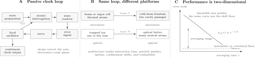
An atomic clock is a closed measurement loop. A: state preparation, interrogation, and readout produce an error signal that disciplines the local oscillator; the oscillator supplies the continuous output. B: thermal or vapor-cell microwave devices, cold-atom fountains, trapped ions, and neutral-atom lattices implement the same logic with different interaction times and particle numbers. C: white frequency noise averages approximately as $\tau^{-1/2}$ until a systematic or correlated noise floor is reached; a narrow line alone determines neither curve.

The atomic package is therefore a frequency discriminator embedded in a control system. Its resonance may be extraordinarily reproducible, but the clock inherits every phase perturbation between oscillator synthesis, interrogation, atoms, and detection.

Choosing a Clock Transition

Frequency and quality factor

For an observed linewidth $\Delta\nu$, define the spectroscopic quality factor

$$Q = \frac{\nu_0}{\Delta\nu}.$$

If the line-center signal-to-noise ratio and cycle time were otherwise equal, a larger $Q$ would provide a steeper fractional-frequency discriminator. Interrogating a transition near $5\times10^{14}\ \mathrm{Hz}$ with a $1\ \mathrm{Hz}$ linewidth gives $Q\sim5\times10^{14}$; a $9.2\ \mathrm{GHz}$ transition with the same linewidth gives $Q\sim9\times10^9$.

This comparison is useful but incomplete. A viable transition also needs:

• a long intrinsic coherence time;
• reproducible state preparation and efficient readout;
• an accessible probe source with adequate phase coherence;
• low sensitivity, or calibratable sensitivity, to magnetic and electric fields;
• controlled motion and confinement;
• manageable collisions and density shifts;
• acceptable spontaneous decay and branching;
• enough particles or detection fidelity for the required stability;
• practical cooling, trapping, repumping, and duty cycle; and
• reliable atomic-structure coefficients for the shift model.

A transition can have a spectacular natural $Q$ and still make a poor clock if the probe laser loses coherence first or if the environment shifts the line unpredictably.

Unperturbed and realized frequencies

Write the transition frequency in the apparatus as

$$\nu_{\mathrm{at}} \left( \boldsymbol\lambda \right) = \nu_0 + \sum_i \Delta\nu_i \left( \boldsymbol\lambda \right),$$

where $\boldsymbol\lambda$ collects magnetic fields, electric fields, temperature, density, motion, probe parameters, trap settings, and other controls. Near an operating point,

$$\begin{aligned} \Delta\nu_i &\simeq k_i \left( \lambda_i-\lambda_{i,0} \right), \\ \Delta\nu_j &\simeq k_j^{(2)} \left( \lambda_j-\lambda_{j,0} \right)^2, \end{aligned}$$

for representative linear and quadratic sensitivities. A “clock transition” usually means that one or more first derivatives vanish or are small. It does not mean that all perturbations vanish.

The caesium clock transition

The present SI definition fixes the numerical value of the unperturbed ground-state hyperfine transition frequency of $^{133}\mathrm{Cs}$:

$$\Delta\nu_{\mathrm{Cs}} = 9\,192\,631\,770\ \mathrm{Hz} \qquad \text{exactly}.$$

The operational clock transition connects

$$\begin{aligned} |g\rangle &= |6S_{1/2},F=3,m_F=0\rangle, \\ |e\rangle &= |6S_{1/2},F=4,m_F=0\rangle. \end{aligned}$$

At weak magnetic field, the $m_F=0\leftrightarrow m_F=0$ frequency has no first-order Zeeman shift. A small bias field is nevertheless used to define the quantization axis and spectrally separate unwanted Zeeman components. The clock frequency then has a measurable quadratic Zeeman shift. This is a recurring clock-design principle: remove a dangerous first-order sensitivity, retain controlled fields, and correct the residual even-order term.

Hyperfine Structure derives the $F=3$ and $F=4$ levels, while Zeeman Effect in Atoms derives the weak-field and Breit–Rabi behavior.

Primary and secondary realizations

A primary frequency standard realizes the SI second directly from the caesium defining transition and reports an evaluated uncertainty without calibration against a higher standard of the same quantity. A secondary representation of the second uses another transition whose recommended frequency and uncertainty have been adopted through the international metrology process.

The distinction is institutional as well as physical:

• not every caesium clock is a primary standard;
• a caesium device becomes primary only after a defensible realization and uncertainty evaluation;
• rubidium and several optical transitions can serve as recognized secondary representations;
• “secondary” does not imply lower experimental performance;
• a secondary standard can have smaller internal systematic uncertainty than a caesium realization while its absolute frequency remains connected to the current SI definition.

As reviewed on 25 July 2026, caesium still defines the second. The BIPM list of standard frequencies contains microwave and optical secondary representations, and the redefinition roadmap describes a possible future update, possibly in 2030. A roadmap is not a redefinition.

Interrogation and the Clock Discriminator

Rabi and Ramsey interrogation

A single coherent pulse produces a Rabi line whose Fourier width is set approximately by the pulse duration. Ramsey interrogation uses two coherent interactions separated by a dark interval $T$. The atoms then compare the oscillator phase at two times.

For ideal $\pi/2$ pulses and a consistent phase convention, a useful Ramsey model is

$$P_e(\delta\nu) = \frac12 \left[ 1 + C \cos \left( 2\pi\delta\nu T+\phi_c \right) \right],$$

where

$$\delta\nu = \nu_{\mathrm{LO}}-\nu_{\mathrm{at}},$$

$C$ is contrast, and $\phi_c$ includes controlled and systematic phase. The fringe spacing is $1/T$. For the ideal cosine fringe, the central feature has a half-contrast full width

$$\Delta\nu_{\mathrm{FWHM}} \simeq \frac{1}{2T}.$$

Longer dark time narrows the discriminator, but only while atomic coherence and oscillator phase prediction remain adequate. Finite pulses, decoherence, pulse-area errors, phase transients, and multilevel structure modify the simple expression. Their derivation belongs to Ramsey Interferometry.

A two-point error signal

A servo cannot lock robustly to the top of a symmetric fringe because the slope vanishes there. Instead, interrogate at offsets

$$\delta\nu_\pm = \delta\nu \pm \delta_m,$$

and define

$$\mathcal E = P_e(\delta\nu_+) - P_e(\delta\nu_-).$$

Choose

$$\delta_m = \frac{1}{4T},$$

so the two samples lie near opposite half-height slopes. For $\phi_c=0$,

$$\mathcal E = -C \sin \left( 2\pi\delta\nu T \right) \simeq -2\pi C T\,\delta\nu.$$

With this sign convention, a digital integrator can update

$$\nu_{\mathrm{LO}}^{(n+1)} = \nu_{\mathrm{LO}}^{(n)} + G\mathcal E_n, \qquad G>0.$$

If the oscillator is high, $\delta\nu>0$, then $\mathcal E<0$ and the update lowers it. A laboratory must verify this sign with a deliberate frequency step; an elegant servo with the wrong sign locks only by accident or runs away.

Normalization and offset rejection

Atom number and detection gain can vary between the two samples. A normalized discriminator such as

$$\mathcal E_N = \frac{ P_+-P_- }{ P_++P_- }$$

can reject common multiplicative fluctuations, but it also changes the noise statistics and becomes unstable when the denominator is small. Alternating the order of $+$ and $-$ samples, reversing phase steps, and using auxiliary population channels help separate detuning from drift.

A two-point lock is vulnerable to line asymmetry. If the two line wings respond differently to neighboring transitions, pulse area, detection efficiency, or cavity phase, $\mathcal E=0$ need not coincide with the unperturbed line center.

Servo dynamics

The atomic measurement is sampled and noisy. A practical servo must choose:

• loop gain and bandwidth;
• integral and proportional terms;
• modulation depth;
• update cadence;
• filters and outlier handling;
• integrator limits and relock logic;
• feedforward for predictable drift; and
• a way to preserve raw error and actuator records.

High gain can follow atom noise or become unstable after cycle delay. Low gain leaves residual local-oscillator drift and servo error. The in-loop error can look quiet because feedback suppresses it; an independent clock, out-of-loop beat, or interleaved configuration is needed to validate the actual output.

The clock cycle matters

If interrogation occupies time $T$ in a total cycle $T_c$, the duty factor is roughly

$$d = \frac{T}{T_c}.$$

Loading, cooling, state preparation, detection, and computation create dead time. Dead time reduces the number of measurements and makes the sampled atomic discriminator sensitive to aliased local-oscillator noise. It is therefore a physical parameter, not merely an implementation overhead.

Microwave Clocks

Microwave clocks generally use ground-state hyperfine transitions. Their oscillators and electronics are mature, and compact implementations can run continuously for years. The principal architectures trade interaction time, size, power, stability, and evaluability.

Thermal caesium beam

A classical caesium beam standard sends atoms from an oven through:

1. state selection;
2. a first microwave interaction zone;
3. a free-flight region;
4. a second interaction zone; and
5. state-selective detection.

Separated fields give Ramsey narrowing. Thermal velocity limits the dark time, while a velocity distribution averages different transit phases and second-order Doppler shifts. Cavity phase, microwave power, state-selection asymmetry, and line pulling require control.

Beam standards are robust and can operate continuously. Historically they made atomic time practical, and commercial devices remain useful as holdover and ensemble clocks. A commercial caesium beam clock is not automatically a primary realization because its complete correction model is generally not evaluated at the level of a national primary standard.

Rubidium and caesium vapor cells

Vapor-cell clocks confine alkali atoms in a sealed cell. Buffer gas, anti-relaxation wall coatings, or both extend coherence by slowing diffusion to the walls. Optical pumping prepares the atoms and optical absorption or fluorescence reads out the microwave resonance.

Compact clocks often use coherent population trapping (CPT). Two optical frequency components separated by the ground-state hyperfine frequency create a dark state. The microwave-frequency difference is then interrogated without a conventional microwave cavity.

Advantages include small size, low power, low cost, and continuous operation. Important shifts include:

• buffer-gas pressure and temperature;
• wall interactions and cell aging;
• light shift and optical-power drift;
• laser detuning and spectral sidebands;
• magnetic field;
• microwave leakage or modulation phase;
• spin exchange; and
• electronics and resonator temperature.

These devices optimize deployability and holdover rather than the smallest possible systematic uncertainty. “Atomic” does not mean environmentally insensitive.

Hydrogen masers

The hydrogen maser uses the $1.420\ \mathrm{GHz}$ ground-state hyperfine transition of atomic hydrogen. State-selected atoms enter a storage bulb inside a microwave cavity. Stimulated emission sustains an active oscillation.

Hydrogen masers provide excellent short- and medium-term stability and are valuable flywheels in laboratory time scales and radio astronomy. Their output is affected by cavity pulling, wall shift, spin-exchange effects, magnetic field, atomic flux, and long-term drift. They complement rather than replace evaluated caesium primary standards: the maser carries a smooth phase, while primary or secondary standards calibrate its long-term rate.

Laser-cooled caesium fountains

A fountain replaces a hot beam with a laser-cooled cloud:

1. capture and cool $^{133}\mathrm{Cs}$ atoms;
2. launch the cloud vertically;
3. prepare the clock state;
4. cross a microwave cavity on the upward trajectory;
5. evolve ballistically;
6. cross the same cavity on the downward trajectory; and
7. detect the two hyperfine populations.

For an effective separation near $T=0.5\ \mathrm{s}$,

$$\Delta\nu_{\mathrm{FWHM}} \simeq 1\ \mathrm{Hz},$$

so

$$Q_{\mathrm{Cs}} \simeq \frac{ 9.1926\times10^9\ \mathrm{Hz} }{ 1\ \mathrm{Hz} } \simeq 9.2\times10^9.$$

The same cavity supplies both Ramsey interactions, and the reversal of vertical velocity suppresses some phase errors. It does not cancel everything. Real fountains evaluate:

• quadratic Zeeman shift;
• blackbody radiation shift;
• cold collisions and cavity pulling;
• distributed cavity phase;
• microwave lensing;
• leakage fields and spectral impurities;
• residual first- and second-order Doppler effects;
• state preparation and detection;
• background-gas collisions; and
• relativistic gravitational potential.

The launch height, atom density, cavity geometry, magnetic shielding, temperature map, microwave spectrum, and atomic trajectories all enter the realization.

Microwave architecture comparison

Architecture	Atomic interaction	Principal strength	Characteristic limitations
thermal caesium beam	separated microwave zones in a hot beam	continuous, robust operation	short transit, velocity distribution, cavity phase
vapor-cell Rb or Cs	microwave or CPT resonance in a sealed cell	compact, low power, high availability	light, buffer-gas, wall, temperature, and aging shifts
active hydrogen maser	stimulated microwave emission from stored H	excellent flywheel stability	cavity pulling, wall shift, drift
cold-atom fountain	Ramsey interrogation of launched cold Cs or Rb	long interaction and evaluable systematics	intermittent cycle, collisions, cavity phase, apparatus complexity

No row is universally “best.” A telecommunications node, spacecraft, primary metrology laboratory, and very-long-baseline interferometer impose different size, uptime, phase-noise, and uncertainty requirements.

Optical Clocks

Why move to optical frequency?

Optical clock transitions lie near

$$\nu_0 \sim 10^{14} \text{--} 10^{15}\ \mathrm{Hz},$$

roughly four to five orders of magnitude above microwave hyperfine frequencies. For a fixed absolute frequency uncertainty $\sigma_\nu$, the fractional uncertainty is

$$\sigma_y = \frac{\sigma_\nu}{\nu_0}.$$

A high carrier therefore converts the same absolute line-center resolution into a smaller fractional error. Long-lived forbidden or weakly allowed transitions also provide very high $Q$.

The gain is not free. Optical cycles cannot be counted directly by ordinary electronics, the probe laser must preserve phase over the interrogation, and atoms must be confined without introducing larger shifts.

Confinement and the Lamb–Dicke regime

Optical wavelength makes first-order Doppler sensitivity severe for freely moving thermal atoms. Clocks instead confine ions in radio-frequency or Penning traps, or neutral atoms in optical lattices. Tight confinement can place the motion in the Lamb–Dicke regime, where the spatial extent is small compared with the probe wavelength and first-order Doppler broadening is suppressed.

Confinement introduces new systematics:

• ion micromotion and secular-motion time dilation;
• electric quadrupole shifts;
• trap radio-frequency Stark shifts;
• lattice AC Stark shifts;
• tunneling and motional sidebands;
• density and collisional shifts; and
• spatially varying probe and trapping fields.

The clock is improved only when the confinement perturbation is more controllable than the motion it removes.

Trapped-ion clocks

A trapped-ion clock interrogates one ion or a small ion crystal. Strong confinement, resolved sidebands, and near-unit state-detection fidelity permit exceptional systematic control. Representative clock lines include electric-quadrupole, electric-octupole, and hyperfine-induced transitions.

The small particle number makes quantum projection noise comparatively large. Logic spectroscopy can transfer the state of a difficult clock ion to a co-trapped logic ion for cooling and readout, but then mode coupling, micromotion, sympathetic cooling, and logic operations enter the evidence chain.

Ion Traps develops confinement, secular motion, and micromotion.

Neutral-atom lattice clocks

An optical lattice clock interrogates many neutral atoms confined near an operational or magic wavelength where the differential AC Stark shift of the two clock states is strongly suppressed. Alkaline-earth-like atoms such as strontium and ytterbium provide narrow $^1S_0\leftrightarrow{}^3P_0$ transitions.

Many atoms improve short-term stability approximately as $1/\sqrt N$ for independent particles. The ensemble also introduces density shifts, lattice inhomogeneity, line pulling, collective effects, and requirements on spin polarization and atom-number control.

Optical Lattices owns band structure, recoil scales, and trapping physics. AC Stark Shift and Dynamic Polarizability own the underlying light-shift theory.

Optical local oscillators and combs

The atomic transition is often narrower than the free-running laser. A typical optical clock first stabilizes a laser to a high-finesse reference cavity, then uses the atoms to correct the cavity-stabilized laser at low frequency. Thermal noise, vibration, drift, residual amplitude modulation, and optical-path phase noise all affect the interrogation.

A self-referenced frequency comb maps the locked optical frequency to radio-frequency signals:

$$\nu_n = n f_{\mathrm{rep}} + f_{\mathrm{CEO}}.$$

The comb transfers and divides phase; it does not supply the atomic accuracy. Tooth index, beat sign, carrier-envelope offset, repetition rate, cycle slips, counter synchronization, and path stabilization must all be validated. The complete derivation belongs to Frequency Combs.

Ion and lattice trade-offs

Property	Trapped ion	Neutral-atom lattice
particle number	one or a few	tens to thousands
state readout	often near unit fidelity	ensemble population
projection-noise averaging	slower for one ion	faster with many independent atoms
confinement systematics	micromotion, secular motion, quadrupole shift	lattice Stark, tunneling, density, inhomogeneity
collisional effects	usually small for one ion	central part of the ledger
technical complexity	ion loading, trap fields, cooling, possibly logic ion	cooling stages, lattice, spin preparation, atom-number control
strongest use	individual-particle control and low systematic shifts	rapid averaging and clock networks

This table is architectural, not a ranking. Species choice can reverse individual advantages.

Present metrological status

Optical standards can achieve lower evaluated systematic uncertainties and better comparison stability than caesium fountains. Several optical transitions are internationally recognized secondary representations of the second. As of 25 July 2026, however, the SI definition itself still fixes $\Delta\nu_{\mathrm{Cs}}$.

Statements about a future optical definition should specify:

• the date and version of the governing recommendation;
• whether the statement concerns a roadmap, a proposal, or an adopted resolution;
• the candidate transition or ensemble rule;
• continuity with the existing second;
• comparison and reliability criteria; and
• how multiple species and laboratories establish consistency.

“Optical clocks are more precise” is not a definition.

Stability, Uncertainty, and Time Error

Fractional frequency

Relative to a nominal or reference frequency, define

$$y(t) = \frac{ \nu_{\mathrm{out}}(t)-\nu_{\mathrm{ref}}(t) }{ \nu_{\mathrm{ref}}(t) }.$$

The fractional frequency averaged over an interval of duration $\tau$ is

$$\overline y_k(\tau) = \frac{1}{\tau} \int_{t_k}^{t_k+\tau} y(t)\,dt.$$

The Allan variance is

$$\sigma_y^2(\tau) = \frac12 \left\langle \left[ \overline y_{k+1}(\tau) - \overline y_k(\tau) \right]^2 \right\rangle.$$

For white frequency noise,

$$\sigma_y(\tau) \propto \tau^{-1/2}.$$

This scaling cannot be extrapolated through a drift, flicker floor, step, servo transient, or systematic change. Allan deviation also describes a comparison: the measured result contains both clocks and the transfer link unless one contribution is independently negligible or separated by a model.

Quantum projection-noise benchmark

At Ramsey midfringe, $N$ independent two-level atoms with contrast $C$ have approximately

$$\sigma_P \simeq \frac{1}{2\sqrt N}.$$

Since the ideal fringe slope is

$$\left| \frac{\partial P_e}{\partial\nu} \right| \simeq \pi C T,$$

the single-cycle frequency uncertainty is

$$\sigma_\nu \simeq \frac{ 1 }{ 2\pi C T\sqrt N }.$$

For independent cycles of duration $T_c$,

$$\sigma_y^{\mathrm{QPN}}(\tau) \simeq \frac{ 1 }{ 2\pi\nu_0 C T\sqrt N } \sqrt{ \frac{T_c}{\tau} }.$$

The numerical prefactor depends on line shape, modulation, estimator, and whether one or several cycles form an error sample. The formula is a benchmark, not a performance guarantee.

Worked comparison

Consider three idealized Ramsey clocks:

Parameter	Cs fountain	optical ion	optical lattice
$\nu_0$	$9.1926\times10^9\ \mathrm{Hz}$	$4.29\times10^{14}\ \mathrm{Hz}$	$4.29\times10^{14}\ \mathrm{Hz}$
$N$	$10^6$	$1$	$10^3$
$T$	$0.50\ \mathrm{s}$	$0.50\ \mathrm{s}$	$0.50\ \mathrm{s}$
$T_c$	$1.50\ \mathrm{s}$	$1.00\ \mathrm{s}$	$1.00\ \mathrm{s}$
$C$	$0.90$	$0.90$	$0.90$

The ideal one-second benchmarks are

$$\begin{aligned} \sigma_{y,\mathrm{Cs}}(1\ \mathrm s) &\simeq 4.7\times10^{-14}, \\ \sigma_{y,\mathrm{ion}}(1\ \mathrm s) &\simeq 8.2\times10^{-16}, \\ \sigma_{y,\mathrm{lat}}(1\ \mathrm s) &\simeq 2.6\times10^{-17}. \end{aligned}$$

The optical carrier outweighs the fountain’s larger atom number in this chosen example, and the lattice gains another $\sqrt{1000}$. Actual clocks may be limited by local-oscillator noise, detection, dead time, imperfect contrast, density shifts, or systematics before reaching these values. The example compares architecture scaling, not records.

Local-oscillator noise

Between atomic measurements, the clock output follows the local oscillator. Its phase noise can:

• reduce Ramsey contrast;
• cause cycle slips to adjacent fringes;
• broaden the discriminator;
• add servo error;
• be aliased by periodic sampling; and
• dominate clock comparisons even when atom projection noise is small.

The oscillator must remain predictable enough that the servo knows which fringe to address. A longer interrogation improves ideal resolution but narrows capture range and demands greater phase coherence.

The Dick effect

Let $g(t)$ be the clock’s sensitivity to a small oscillator-frequency perturbation during one cycle, and define

$$g_m = \frac{1}{T_c} \int_0^{T_c} g(t) e^{-i2\pi m t/T_c} \,dt.$$

For a stated one-sided fractional-frequency noise spectrum $S_y(f)$, a common Dick-effect convention gives

$$\sigma_{y,\mathrm{Dick}}^2(\tau) = \frac{1}{\tau} \sum_{m=1}^{\infty} \left| \frac{g_m}{g_0} \right|^2 S_y \left( \frac{m}{T_c} \right).$$

Periodic sensitivity samples local-oscillator noise at harmonics of the cycle frequency and aliases it into the clock record. Different spectral density and Fourier conventions move factors of two, so a quantitative budget must state them.

Mitigations include:

• a quieter local oscillator;
• higher duty factor;
• faster loading and detection;
• interleaved ensembles with complementary dead times;
• synchronous comparison using a common oscillator;
• nondestructive or repeated interrogation; and
• protocols designed for a favorable sensitivity function.

Common-mode rejection in a synchronous comparison can reveal the relative atomic stability while hiding noise that an independent clock would see. Both statements can be useful, but they are not the same claim.

Instability is not systematic uncertainty

Suppose a comparison averages as

$$\sigma_y(\tau) = \frac{ 3\times10^{-16} }{ \sqrt{\tau/(1\ \mathrm s)} }.$$

At $\tau=10^4\ \mathrm s$, the statistical comparison reaches $3\times10^{-18}$. This says nothing by itself about a static $2\times10^{-17}$ blackbody correction uncertainty. Conversely, a clock with a $10^{-18}$ systematic budget may require substantial averaging before a comparison resolves that level.

A mature claim reports:

1. the instability curve and estimator;
2. the averaging interval and data selection;
3. the systematic corrections and covariance;
4. the comparison reference and transfer link;
5. the point at which statistical and systematic uncertainties are combined; and
6. any unresolved drift or nonstationarity.

From frequency error to time error

The clock time offset $x(t)$ obeys

$$x(t)-x(0) = \int_0^t y(t')\,dt'.$$

A constant fractional frequency offset $y_0$ accumulates

$$\Delta x = y_0\Delta t.$$

Thus $y_0=10^{-15}$ produces about $86\ \mathrm{ps}$ in one day and $32\ \mathrm{ns}$ in one year. Quoting “one second in so many years” assumes a constant offset and conceals noise type, calibration cadence, uptime, and relativistic conditions. Allan deviation and a systematic uncertainty budget are more informative.

Systematic-Shift Ledger

Correction model

Let the servo return an observed line-center estimate $\widehat\nu_{\mathrm{obs}}$. A correction model is

$$\widehat\nu_0 = \widehat\nu_{\mathrm{obs}} - \sum_i \widehat{\Delta\nu}_i.$$

In fractional form,

$$\widehat y_0 = \widehat y_{\mathrm{obs}} - \sum_i \widehat c_i.$$

If the corrections have covariance matrix $U_c$ and sensitivity vector $\boldsymbol a$, then

$$u_{\mathrm{sys}}^2 = \boldsymbol a^{\mathsf T} U_c \boldsymbol a.$$

For corrections already expressed in output units, $\boldsymbol a=(1,\ldots,1)^{\mathsf T}$. Treating every entry as independent when temperature, field, atomic coefficients, or calibrations are shared can understate or overstate the final uncertainty.

A cross-platform ledger

Effect	Representative dependence	Microwave emphasis	Optical emphasis	Validation
Zeeman	$k_1B+k_2B^2+\cdots$	bias-field map, quadratic clock shift	linear averaging, quadratic shift	vary $B$, compare Zeeman components
DC Stark	$-\Delta\alpha(0)E^2/(2h)$	usually small but patch fields matter	trap and stray electric fields	electrode reversal, field compensation
blackbody Stark	approximately $T^4$ with dynamic correction	Cs blackbody correction	often a leading optical term	calibrated thermometry, emissivity and view-factor model
probe AC Stark	intensity and detuning	microwave leakage and power	optical probe shift, hyper-Ramsey variants	power and pulse-sequence interleaving
trap or lattice Stark	trap parameters	usually absent in beams and fountains	central lattice or ion-trap term	depth extrapolation, operational wavelength
collisions	density and internal state	cold-collision fountain shift	lattice density and interaction shift	density interleaving, state control
motion	Doppler and $-\langle v^2\rangle/(2c^2)$	thermal beam and fountain trajectories	secular motion, micromotion, recoil	sideband thermometry, trajectory reversal
line pulling	neighboring lines and asymmetry	Zeeman components, cavity spectrum	motional sidebands, unwanted transitions	polarization and population reversals
servo	gain, modulation, drift	synthesis and microwave chain	laser drift, cycle slips, path phase	modulation reversal, independent beat
gravity	$\Delta U/c^2$	primary-standard reference potential	essential near $10^{-18}$	geodetic survey and potential model

The table is a checklist, not a universal budget. Terms that are negligible for one species can dominate another.

Magnetic shifts

For a first-order-insensitive clock state,

$$\Delta\nu_Z \simeq k_Z B^2.$$

For the caesium $m_F=0\leftrightarrow m_F=0$ transition near weak field,

$$k_Z \simeq 427.45\ \mathrm{Hz\,G^{-2}}.$$

At $B=1.0\ \mathrm{mG}$, this is

$$\Delta\nu_Z \simeq 4.27\times10^{-4}\ \mathrm{Hz},$$

or a fractional shift near

$$\frac{\Delta\nu_Z}{\nu_{\mathrm{Cs}}} \simeq 4.65\times10^{-14}.$$

The shift is far larger than a fountain’s target uncertainty and must be corrected. Field-insensitive means reduced derivative, not negligible correction.

Clock experiments infer the field from magnetically sensitive transitions, map it along trajectories, reverse or vary coil current, and propagate the coefficient and field uncertainties. Since $\Delta\nu_Z\propto B^2$, a small relative field uncertainty contributes approximately twice that relative uncertainty to the shift when coefficient uncertainty is negligible.

Electric and blackbody shifts

For a static electric field,

$$\Delta\nu_{\mathrm{DC}} = -\frac{ \Delta\alpha(0) }{ 2h } E^2,$$

where $\Delta\alpha(0)$ is the differential static polarizability. Thermal radiation produces an AC Stark shift that is often organized as

$$\Delta\nu_{\mathrm{BBR}}(T) = -\frac{ \Delta\alpha(0) }{ 2h } \langle E^2(T)\rangle \left[ 1+\eta(T) \right],$$

with

$$\langle E^2(T)\rangle \propto T^4$$

and dynamic correction $\eta(T)$.

The relevant temperature is the radiation field seen by the atoms, not automatically one convenient sensor. Windows, ovens, electrodes, trap structures, emissivity, and view factors can create a nonuniform environment. Validation uses multiple calibrated sensors, thermal models, deliberate temperature changes, and agreement with independent polarizability information.

Probe and trapping light

An optical probe or lattice changes the levels it measures. The shift can depend on intensity, polarization, detuning, pulse sequence, motional state, and higher-order polarizability. A magic wavelength cancels the leading differential polarizability under specified conditions; multipolar, hyperpolarizability, detuning, and thermal-motion terms remain.

Useful tests include:

• interleaving high and low intensity;
• reversing polarization or magnetic sublevel;
• varying pulse duration at fixed pulse area;
• changing lattice depth and wavelength independently;
• comparing Rabi, Ramsey, and shift-suppressing sequences; and
• verifying the extrapolated zero or operational point on held-out data.

Collisions and density

Interactions shift the clock frequency through state-dependent scattering and exchange. In a fountain, the cold-collision shift is commonly measured by alternating high and low density and extrapolating to zero density. The two samples must differ only in density; changing spatial distribution, temperature, state composition, or trajectory can corrupt the slope.

In lattice clocks, quantum statistics, spin polarization, site occupancy, excitation fraction, tunneling, and interaction inhomogeneity matter. “Fermions do not collide” is not an acceptable shift model.

Motion and relativity

Residual first-order Doppler phase can arise from wavefronts, cavity phase, optical-path motion, or asymmetric trajectories even when the mean atomic velocity is small. Special-relativistic time dilation contributes

$$\frac{\Delta\nu_{\mathrm{TD}}}{\nu_0} = -\frac{ \langle v^2\rangle }{ 2c^2 }.$$

For trapped ions, secular motion and driven micromotion both enter. For neutral lattices, sideband thermometry and band populations constrain motion. For thermal beams, the velocity distribution and line shape must be modeled. For fountains, launch tilt and cavity phase couple trajectory to frequency.

Fountain-specific microwave shifts

Three effects deserve separate names:

• Distributed cavity phase: the microwave phase is not spatially uniform; atoms sample different phase on the upward and downward passes.
• Microwave lensing: gradients of the standing microwave field exert state-dependent dipole forces and alter detected trajectories.
• Microwave leakage: fields outside the intended Ramsey interactions add phase with timing and amplitude not represented by the ideal sequence.

Tests include changing cavity feed balance, reversing launch direction where possible, mapping trajectories, changing microwave amplitude, modifying timing, and comparing detailed electromagnetic and atomic-trajectory models.

Line pulling and servo shifts

Neighboring Zeeman, motional, or hyperfine components can pull a fitted line center when their populations or shapes are asymmetric. Probe phase transients can create an offset that looks like detuning. Slow local- oscillator drift combined with sequential sampling can create servo error.

Diagnostic reversals include:

• swap the order of high- and low-frequency samples;
• reverse the phase-step sign;
• change modulation depth;
• alternate magnetic sublevels;
• reverse polarization;
• vary pulse area;
• compare independent line-shape models; and
• inject a known synthetic frequency step.

The correction should be supported by a response model and variation data, not by the claim that a servo is locked.

Gravitational redshift

Clocks at different gravitational potentials have different proper rates:

$$\frac{\Delta\nu}{\nu} \simeq \frac{\Delta U}{c^2}.$$

Near Earth’s surface, the uniform-field estimate is

$$\frac{\Delta\nu}{\nu} \simeq \frac{g\,\Delta h}{c^2} \simeq 1.09\times10^{-16} \left( \frac{\Delta h}{1\ \mathrm m} \right).$$

At $10^{-18}$, centimetre-scale height differences matter. A metrological correction uses gravitational potential, reference conventions, tides, local gravity, and a geodetic survey, not only a ruler and constant $g$.

Worked correction budget

Suppose a clock comparison reports

$$y_{\mathrm{obs}} = 42.0\times10^{-16}.$$

The evaluated fractional shifts, in units of $10^{-16}$, are:

Effect	Shift $c_i$	Standard uncertainty $u_i$
quadratic Zeeman	$+7.0$	$0.3$
blackbody radiation	$-16.5$	$0.5$
density	$+2.0$	$0.8$
interrogation and servo	$+0.5$	$0.4$
relativistic reference	$+4.0$	$0.2$

The summed shift is

$$\sum_i c_i = -3.0\times10^{-16},$$

so the corrected result is

$$y_0 = y_{\mathrm{obs}} - \sum_i c_i = 45.0\times10^{-16}.$$

If the entries are independent,

$$\begin{aligned} u_{\mathrm{sys}} &= \sqrt{ 0.3^2+0.5^2+0.8^2+0.4^2+0.2^2 } \times10^{-16} \\ &= 1.09\times10^{-16}. \end{aligned}$$

With a statistical standard uncertainty $u_{\mathrm{stat}}=1.50\times10^{-16}$,

$$u_{\mathrm{tot}} = \sqrt{ u_{\mathrm{stat}}^2 + u_{\mathrm{sys}}^2 } = 1.85\times10^{-16}.$$

If blackbody and relativistic corrections share temperature or geometry inputs, or several shifts share one field calibration, covariance must be included. The arithmetic is the final step; validating each entry is the substantive work.

Validating a Clock

Interleaved evaluations

To measure a shift coefficient, alternate two values of a control parameter faster than relevant drift:

$$\widehat k = \frac{ \widehat\nu(\lambda_2) - \widehat\nu(\lambda_1) }{ \lambda_2-\lambda_1 }.$$

Interleaving cancels common drift only to the extent that drift is common and sampled symmetrically. The two conditions must not change hidden variables such as atom number, temperature, trajectory, linewidth, or detection gain.

Reversal parity

Many desired or nuisance signals have known symmetry. If a control $s=\pm1$ is reversed, decompose

$$\begin{aligned} \nu_{\mathrm{even}} &= \frac{ \nu(+1)+\nu(-1) }{2}, \\ \nu_{\mathrm{odd}} &= \frac{ \nu(+1)-\nu(-1) }{2}. \end{aligned}$$

Magnetic-sublevel averaging, field reversal, propagation reversal, and polarization reversal can isolate different parity channels. Imperfect reversal leaks even terms into odd channels, so reversal fidelity belongs in the model.

Independent comparisons

One clock cannot establish its own accuracy from a quiet in-loop error signal. Strong evidence comes from:

• comparison with another clock of the same species;
• comparison with a different species and different sensitivities;
• direct optical ratios that bypass part of a microwave chain;
• remote comparison over an independently characterized link;
• redundant combs or synthesis chains;
• agreement of repeated evaluations after apparatus changes; and
• blind or withheld analysis choices for high-stakes tests.

Agreement is interpreted through combined uncertainty. Disagreement is diagnostic; averaging inconsistent results is not a repair.

Closure tests

For three clock frequencies,

$$R_{AB} = \frac{\nu_A}{\nu_B}, \qquad R_{BC} = \frac{\nu_B}{\nu_C}, \qquad R_{CA} = \frac{\nu_C}{\nu_A},$$

ideal closure requires

$$R_{AB}R_{BC}R_{CA} = 1.$$

The logarithmic residual

$$\epsilon_{\mathrm{cl}} = \ln R_{AB} + \ln R_{BC} + \ln R_{CA}$$

tests the combined clocks and comparison chain. Shared references and correlations must be retained when its uncertainty is calculated.

Architecture Selection

Choose an architecture from the measurement requirement, not from one headline number.

Requirement	Often favorable architecture	Reason
low size, weight, and power	vapor-cell or chip-scale clock	compact package and modest electronics
autonomous holdover	rubidium, caesium beam, or maser ensemble	continuous operation and mature reliability
smooth short-term phase	hydrogen maser or ultrastable cavity flywheel	low short-term phase noise
direct realization of present SI second	evaluated caesium primary standard	defining transition
smallest optical systematic uncertainty	selected trapped-ion or lattice clock	high carrier and controlled confinement
rapid optical averaging	many-atom lattice clock	large $N$
transportable relativistic survey	transportable optical or cold-atom clock	high sensitivity with engineered portability
robust network node	redundant ensemble with transfer monitoring	uptime and fault tolerance

The best system may be an ensemble: a maser or commercial clock supplies continuous phase, an optical or caesium standard periodically calibrates rate, and a time-scale algorithm combines them. Frequency accuracy, phase continuity, availability, and maintainability are distinct design axes.

A Reproducible Clock Workflow

1. Specify the measurand. State isotope, transition, sublevels, unperturbed convention, reference frame, and gravitational potential.
2. Write the frequency chain. Identify the local oscillator, synthesizers, comb coordinates, beat signs, counters, and output plane.
3. Define the interrogation. Record pulse phases, durations, dark time, detuning convention, cycle time, and sensitivity function.
4. Calibrate preparation and readout. Measure state fidelity, contrast, atom number, detection nonlinearity, and background.
5. Verify the discriminator. Apply signed frequency steps, reverse the modulation, and map the capture range.
6. Characterize the servo. Record loop gain, update rule, drift feedforward, integrator state, cycle slips, and relocks.
7. Measure instability. Preserve raw phase or frequency data, state the estimator and dead-time treatment, and compare against an independent reference.
8. Build the shift ledger. Give each correction a model, data set, coefficient, uncertainty, covariance, and validity range.
9. Run reversals and interleaves. Change one physical parameter at a time and monitor correlated auxiliary variables.
10. Correct relativity and transfer. State the potential reference, link model, counter synchronization, and path-noise correction.
11. Perform closure. Use another species, clock, comb, or transfer path when the claimed level warrants it.
12. Freeze and report. Preserve software, calibration versions, exclusions, uncertainty calculations, and the date-sensitive SI status.

Common Mistakes

Saying that an atom ticks by itself

The useful output of a passive clock is a local oscillator disciplined by probabilistic atomic measurements.

Equating linewidth with uncertainty

Linewidth controls resolution and discriminator slope. The line center can still be shifted, and estimator variance depends on signal-to-noise ratio and sampling.

Calling every caesium clock primary

Primary status requires direct realization of the defining transition with an evaluated correction and uncertainty budget.

Calling every optical clock more accurate

High optical frequency improves fractional leverage. Actual uncertainty depends on species, apparatus, evaluation, and comparison evidence.

Treating a clock transition as field free

Suppressing first-order Zeeman or Stark sensitivity leaves quadratic and higher-order terms, as well as unrelated shifts.

Ignoring the local oscillator

Probe coherence, path phase, dead time, and servo dynamics can dominate even when the atomic transition is exceptionally narrow.

Extrapolating white-noise scaling indefinitely

Drift, flicker noise, environmental changes, and systematic floors prevent unlimited $\tau^{-1/2}$ averaging.

Using an in-loop error as independent evidence

Feedback suppresses the error signal it observes. Out-of-loop comparison is needed to establish output performance.

Forgetting covariance

Shared temperature, field, atomic coefficients, transfer links, or references correlate shift entries and clock comparisons.

Converting uncertainty to “years per second” without assumptions

That slogan treats a fractional uncertainty as a constant deterministic rate and hides uptime, noise type, and calibration.

Calling the planned redefinition complete

As of 25 July 2026, caesium remains the SI defining transition. Optical secondary representations and a redefinition roadmap do not alter that fact.

Further Connections

• Atomic Clocks for Quantum Estimation treats the clock as a partially observed dynamical system and audits quantum gain after oscillator noise, dead time, feedback, and global reliability.
• Ramsey Interferometry for Quantum Estimation develops binary likelihoods, local information, phase unwrapping, interrogation-time design, and duty-cycle accounting.
• Spin Squeezing owns the collective-spin parameters, preparation mechanisms, entanglement criteria, and matched-clock-gain audit used by squeezing-enhanced clocks.
• Precision Measurement and Metrology develops the generic measurement chain, covariance model, projection-noise benchmark, and evidence ledger.
• Optical Clocks develops narrow optical references, trapped-ion and lattice architectures, comb comparisons, systematics, geodesy, and frequency-ratio tests.
• Frequency Standards develops realization hierarchies, Allan-family statistics, UTC($k$), TAI, transfer links, and metrological traceability.
• AMO Experiment Index connects Ramsey interrogation, the first cesium standard, modern optical clocks, and the present SI status in a milestone-oriented evidence table.
• Variation of Constants Searches develops the sensitivity-coefficient, signal-template, and trials-aware analysis used to interpret long clock-comparison records.
• Ramsey Interferometry derives the separated-pulse fringe, finite-pulse corrections, and phase sensitivity used by many clocks.
• Rabi Oscillations develops pulse calibration and single-pulse spectroscopy.
• Precision Spectroscopy develops line-center inference, uncertainty budgets, and frequency-ratio tests.
• Frequency Combs develops optical counting, transfer oscillators, and coherent division.
• Laser Stabilization develops reference cavities, error signals, loop transfer functions, and out-of-loop validation.
• Hyperfine Structure derives the microwave transitions used by caesium, rubidium, and hydrogen standards.
• Zeeman Effect in Atoms develops clock-state magnetic sensitivities.
• AC Stark Shift and Dynamic Polarizability supply the light-shift framework for optical clocks.
• Ion Traps and Optical Lattices develop the confinement physics behind the two leading optical architectures.
• Quantum Sensing places clock phase estimation in the broader Fisher-information and decoherence framework.

References

1. Bureau International des Poids et Mesures, The International System of Units (SI Brochure), 9th ed., version 4.01 (June 2026), doi:10.59161/AUEZ1291.
2. Bureau International des Poids et Mesures, “Recommended values of standard frequencies: for the second,” updated 2025, BIPM standard-frequency list.
3. Bureau International des Poids et Mesures, “Roadmap to the redefinition of the second,” updated March 2025, BIPM redefinition portal.
4. N. Dimarcq et al., “Roadmap towards the redefinition of the second,” Metrologia 61, 012001 (2024), doi:10.1088/1681-7575/ad17d2.
5. N. F. Ramsey, “A molecular beam resonance method with separated oscillating fields,” Physical Review 78, 695–699 (1950), doi:10.1103/PhysRev.78.695.
6. L. Essen and J. V. L. Parry, “An atomic standard of frequency and time interval: a caesium resonator,” Nature 176, 280–282 (1955), doi:10.1038/176280a0.
7. H. M. Goldenberg, D. Kleppner, and N. F. Ramsey, “Atomic hydrogen maser,” Physical Review Letters 5, 361–362 (1960), doi:10.1103/PhysRevLett.5.361.
8. A. Bauch, “Caesium atomic clocks: function, performance and applications,” Measurement Science and Technology 14, 1159–1173 (2003), doi:10.1088/0957-0233/14/8/301.
9. R. Wynands and S. Weyers, “Atomic fountain clocks,” Metrologia 42, S64–S79 (2005), doi:10.1088/0026-1394/42/3/S08.
10. S. Weyers et al., “Advances in the accuracy, stability, and reliability of the PTB primary fountain clocks,” Metrologia 55, 789–805 (2018), doi:10.1088/1681-7575/aae008.
11. V. Gerginov et al., “Accuracy evaluation of primary frequency standard NIST-F4,” Metrologia 62, 035002 (2025), doi:10.1088/1681-7575/adc7bd; corrected by Metrologia 63, 019502 (2026), doi:10.1088/1681-7575/ae382e.
12. J. Vanier, “Atomic clocks based on coherent population trapping: a review,” Applied Physics B 81, 421–442 (2005), doi:10.1007/s00340-005-1905-3.
13. J. Kitching, “Chip-scale atomic devices,” Applied Physics Reviews 5, 031302 (2018), doi:10.1063/1.5026238.
14. A. D. Ludlow, M. M. Boyd, J. Ye, E. Peik, and P. O. Schmidt, “Optical atomic clocks,” Reviews of Modern Physics 87, 637–701 (2015), doi:10.1103/RevModPhys.87.637.
15. W. M. Itano et al., “Quantum projection noise: population fluctuations in two-level systems,” Physical Review A 47, 3554–3570 (1993), doi:10.1103/PhysRevA.47.3554.
16. G. Santarelli et al., “Frequency stability degradation of an oscillator slaved to a periodically interrogated atomic resonator,” IEEE Transactions on Ultrasonics, Ferroelectrics, and Frequency Control 45, 887–894 (1998), doi:10.1109/58.710548.
17. D. W. Allan, “Statistics of atomic frequency standards,” Proceedings of the IEEE 54, 221–230 (1966), doi:10.1109/PROC.1966.4634.
18. W. J. Riley, Handbook of Frequency Stability Analysis, NIST Special Publication 1065 (2008), doi:10.6028/NIST.SP.1065.
19. F. Riehle, Frequency Standards: Basics and Applications (Wiley-VCH, 2004), doi:10.1002/3527605991.
20. T. L. Nicholson et al., “Systematic evaluation of an atomic clock at $2\times10^{-18}$ total uncertainty,” Nature Communications 6, 6896 (2015), doi:10.1038/ncomms7896.
21. E. Oelker et al., “Demonstration of $4.8\times10^{-17}$ stability at $1\ \mathrm{s}$ for two independent optical clocks,” Nature Photonics 13, 714–719 (2019), doi:10.1038/s41566-019-0493-4.
22. J. Levine, “Introduction to time and frequency metrology,” Review of Scientific Instruments 70, 2567–2596 (1999), doi:10.1063/1.1149844.

Exercises

1. Ramsey linewidth and quality factor

An ideal clock uses a Ramsey dark time $T=0.400\ \mathrm{s}$.

1. Estimate the central-fringe half-contrast FWHM.
2. Find $Q$ for the caesium defining frequency.
3. Find $Q$ for an optical transition at $4.29\times10^{14}\ \mathrm{Hz}$.
4. Explain why the ratio of the two $Q$ values is not by itself the ratio of realized clock uncertainties.

Solution

For the ideal Ramsey cosine,

$$\Delta\nu_{\mathrm{FWHM}} \simeq \frac{1}{2T} = \frac{1}{ 0.800\ \mathrm s } = 1.25\ \mathrm{Hz}.$$

For caesium,

$$Q_{\mathrm{Cs}} = \frac{ 9.192631770\times10^9 }{ 1.25 } \simeq 7.35\times10^9.$$

For the optical transition,

$$Q_{\mathrm{opt}} = \frac{ 4.29\times10^{14} }{ 1.25 } \simeq 3.43\times10^{14}.$$

Their ratio is

$$\frac{Q_{\mathrm{opt}}}{Q_{\mathrm{Cs}}} \simeq 4.67\times10^4.$$

This is the carrier-frequency ratio because the linewidths were chosen equal. Realized uncertainty also depends on particle number, contrast, cycle time, local-oscillator noise, dead time, detection, systematic shifts, and the quality of their evaluation.

2. Determine the lock sign

Use

$$P_e(\delta\nu) = \frac12 \left[ 1+C\cos(2\pi\delta\nu T) \right]$$

and sample at

$$\delta\nu_\pm = \delta\nu \pm \frac{1}{4T}.$$

1. Derive $\mathcal E=P_e(\delta\nu_+)-P_e(\delta\nu_-)$.

2. Linearize near $\delta\nu=0$.

3. For an update

   $$\nu_{\mathrm{LO}}^{(n+1)} = \nu_{\mathrm{LO}}^{(n)} + G\mathcal E_n,$$

   determine the stable sign of $G$.

4. What physical test should be made before closing the loop?

Solution

Let $x=2\pi\delta\nu T$. The modulation phases are $x\pm\pi/2$, so

$$\begin{aligned} \mathcal E &= \frac{C}{2} \left[ \cos(x+\pi/2) - \cos(x-\pi/2) \right] \\ &= \frac{C}{2} \left[ -\sin x-\sin x \right] \\ &= -C\sin x. \end{aligned}$$

Near the lock point,

$$\mathcal E \simeq -2\pi C T\,\delta\nu.$$

If $\delta\nu>0$, the oscillator is high and $\mathcal E<0$. Therefore $G>0$ makes the update negative and supplies restoring feedback under the stated definitions.

Before closing the loop, apply a known positive and negative frequency step and verify the observed discriminator sign. This catches swapped sample labels, frequency-synthesis signs, and phase conventions.

3. Projection-noise-limited architectures

Three idealized clocks have the parameters in the worked comparison:

$$\begin{array}{c|ccc} & \mathrm{Cs} & \mathrm{ion} & \mathrm{lattice} \\ \hline \nu_0\ (\mathrm{Hz}) & 9.1926\times10^9 & 4.29\times10^{14} & 4.29\times10^{14} \\ N & 10^6 & 1 & 10^3 \\ T\ (\mathrm s) & 0.50 & 0.50 & 0.50 \\ T_c\ (\mathrm s) & 1.50 & 1.00 & 1.00 \end{array}$$

All have $C=0.90$.

1. Calculate their ideal $\sigma_y(1\ \mathrm{s})$.
2. Calculate their ideal values at $\tau=10^4\ \mathrm{s}$.
3. Give four reasons an observed comparison may lie above these curves.

Solution

Using

$$\sigma_y(\tau) = \frac{ 1 }{ 2\pi\nu_0 C T\sqrt N } \sqrt{ \frac{T_c}{\tau} },$$

one obtains

$$\begin{aligned} \sigma_{y,\mathrm{Cs}}(1\ \mathrm s) &\simeq 4.7\times10^{-14}, \\ \sigma_{y,\mathrm{ion}}(1\ \mathrm s) &\simeq 8.2\times10^{-16}, \\ \sigma_{y,\mathrm{lat}}(1\ \mathrm s) &\simeq 2.6\times10^{-17}. \end{aligned}$$

At $10^4\ \mathrm{s}$, ideal white-frequency scaling divides each value by $100$:

$$\begin{aligned} \sigma_{y,\mathrm{Cs}} &\simeq 4.7\times10^{-16}, \\ \sigma_{y,\mathrm{ion}} &\simeq 8.2\times10^{-18}, \\ \sigma_{y,\mathrm{lat}} &\simeq 2.6\times10^{-19}. \end{aligned}$$

Observed curves can be higher because of local-oscillator noise and the Dick effect, imperfect contrast, detection noise, atom-number fluctuations, dead time, decoherence, path phase noise, technical environmental noise, or a second clock and transfer link in the comparison. The ideal $\tau^{-1/2}$ extrapolation can also fail at a drift or flicker floor.

4. Quadratic Zeeman correction

Use

$$\Delta\nu_Z = k_ZB^2, \qquad k_Z = 427.45\ \mathrm{Hz\,G^{-2}},$$

for a caesium clock operating at

$$B = 1.20\ \mathrm{mG}.$$

The standard field uncertainty is $u(B)=1.5\ \mathrm{\mu G}$, and the coefficient uncertainty is negligible.

1. Find the shift in hertz.
2. Find the fractional shift.
3. Propagate the field uncertainty.
4. Explain why setting $B=0$ is not necessarily the better operating procedure.

Solution

Since

$$B = 1.20\times10^{-3}\ \mathrm G,$$

the shift is

$$\begin{aligned} \Delta\nu_Z &= 427.45 \left( 1.20\times10^{-3} \right)^2 \mathrm{Hz} \\ &= 6.16\times10^{-4}\ \mathrm{Hz}. \end{aligned}$$

The fractional shift is

$$\frac{\Delta\nu_Z}{\nu_{\mathrm{Cs}}} = \frac{ 6.16\times10^{-4} }{ 9.192631770\times10^9 } \simeq 6.70\times10^{-14}.$$

Linear propagation gives

$$u(\Delta\nu_Z) = 2k_ZB\,u(B).$$

With $u(B)=1.5\times10^{-6}\ \mathrm G$,

$$u(\Delta\nu_Z) \simeq 1.54\times10^{-6}\ \mathrm{Hz},$$

or

$$u_Z \simeq 1.67\times10^{-16}$$

fractionally.

A controlled bias field defines the quantization axis and separates unwanted Zeeman transitions. Near nominal zero, uncontrolled residual fields and spatial direction changes can produce line overlap, Majorana transitions, and poor state definition. The better strategy is a stable, mapped field with a corrected quadratic shift.

5. Dead time and oscillator noise

Clock A interrogates for $T=0.80\ \mathrm{s}$ in a cycle $T_c=1.00\ \mathrm{s}$. Clock B has the same interrogation but $T_c=2.00\ \mathrm{s}$.

1. Find the two duty factors.
2. At equal $\nu_0$, $C$, and $N$, find the ratio of their ideal projection-noise Allan deviations.
3. Which clock is generally more exposed to Dick aliasing?
4. Why can the exact Dick-noise ratio not be found from the duty factors alone?

Solution

The duty factors are

$$d_A = \frac{0.80}{1.00} = 0.80, \qquad d_B = \frac{0.80}{2.00} = 0.40.$$

The QPN benchmark contains $\sqrt{T_c}$, so

$$\frac{ \sigma_{y,B}^{\mathrm{QPN}} }{ \sigma_{y,A}^{\mathrm{QPN}} } = \sqrt{ \frac{T_{c,B}}{T_{c,A}} } = \sqrt2.$$

Clock B generally has stronger aliasing because its dead-time fraction is larger. The exact Dick contribution requires the full sensitivity function $g(t)$ and the local-oscillator noise spectrum at harmonics $m/T_c$. Two protocols with the same duty factor can have different pulse shapes, timing, Fourier coefficients, and oscillator spectra.

6. Correct a shift budget

Use the worked ledger:

$$y_{\mathrm{obs}} = 42.0\times10^{-16},$$

with shifts and uncertainties, in units of $10^{-16}$,

$$\begin{array}{c|cc} & c_i & u_i \\ \hline \mathrm{Zeeman} & 7.0 & 0.3 \\ \mathrm{BBR} & -16.5 & 0.5 \\ \mathrm{density} & 2.0 & 0.8 \\ \mathrm{servo} & 0.5 & 0.4 \\ \mathrm{relativity} & 4.0 & 0.2 \end{array}$$

1. Find the corrected result.
2. Find the independent systematic uncertainty.
3. Combine it with $u_{\mathrm{stat}}=1.50\times10^{-16}$.
4. Now suppose the BBR and relativistic corrections have correlation coefficient $\rho=0.60$. Recalculate the systematic and total uncertainties.

Solution

The shift sum is

$$\sum_i c_i = 7.0-16.5+2.0+0.5+4.0 = -3.0.$$

Therefore

$$y_0 = \left[ 42.0-(-3.0) \right] \times10^{-16} = 45.0\times10^{-16}.$$

Under independence,

$$u_{\mathrm{sys}} = \sqrt{ 0.3^2+0.5^2+0.8^2+0.4^2+0.2^2 } \times10^{-16} = 1.09\times10^{-16}.$$

The total is

$$u_{\mathrm{tot}} = \sqrt{ 1.50^2+1.09^2 } \times10^{-16} = 1.85\times10^{-16}.$$

The covariance contribution is

$$2\rho u_{\mathrm{BBR}}u_{\mathrm{rel}} = 2(0.60)(0.5)(0.2) = 0.12$$

in squared ledger units. Hence

$$u_{\mathrm{sys,corr}} = \sqrt{ 1.18+0.12 } \times10^{-16} = 1.14\times10^{-16},$$

and

$$u_{\mathrm{tot,corr}} = \sqrt{ 1.50^2+1.14^2 } \times10^{-16} = 1.88\times10^{-16}.$$

The corrected central value is unchanged because correlation changes the uncertainty, not the listed corrections.

7. Frequency offset and accumulated time

A continuously running clock has a constant fractional offset

$$y_0 = -2.5\times10^{-15}.$$

1. Find the accumulated time offset after one day.
2. Find it after 30 days.
3. What frequency correction should be applied to a $10\ \mathrm{MHz}$ output?
4. Why is this calculation not a prediction for a clock whose Allan deviation has a flicker floor but whose mean offset is unknown?

Solution

For constant offset,

$$\Delta x = y_0\Delta t.$$

After one day,

$$\Delta x = (-2.5\times10^{-15}) (86\,400\ \mathrm s) = -2.16\times10^{-10}\ \mathrm s,$$

or $-216\ \mathrm{ps}$.

After 30 days,

$$\Delta x = -6.48\times10^{-9}\ \mathrm s,$$

or $-6.48\ \mathrm{ns}$.

The output frequency error is

$$\Delta\nu = y_0\nu_{\mathrm{nom}} = (-2.5\times10^{-15}) (10^7\ \mathrm{Hz}) = -2.5\times10^{-8}\ \mathrm{Hz}.$$

The correcting frequency step is therefore $+2.5\times10^{-8}\ \mathrm{Hz}$ under this sign convention.

A flicker floor describes stochastic frequency behavior, not a known constant mean offset. Its time-error distribution depends on the noise process, observation interval, steering, and initial conditions. One cannot replace that stochastic model by $y_0\Delta t$ without estimating $y_0$.

8. Design an atomic clock

Choose one mission:

• a battery-powered navigation holdover clock;
• a national primary realization of the present SI second;
• a transportable relativistic-geodesy clock;
• a laboratory optical-ratio reference; or
• a very-long-baseline radio-astronomy flywheel.

Propose an architecture and specify:

1. clock species and transition;
2. passive or active operation;
3. local oscillator and output;
4. interrogation and duty cycle;
5. expected leading instability sources;
6. at least eight systematic effects;
7. calibration and reversal tests;
8. comparison and traceability route; and
9. the evidence needed before deployment.

Solution

There is no unique solution. For a national realization of the present SI second, an evaluated $^{133}\mathrm{Cs}$ fountain is the direct architecture. A defensible design includes:

• laser cooling and launch of caesium;
• preparation of $|F=3,m_F=0\rangle$;
• two passages through one microwave Ramsey cavity;
• state-selective fluorescence detection;
• a low-phase-noise microwave oscillator, synthesis chain, and digital servo;
• a continuously running maser or clock ensemble as phase flywheel; and
• transfer to a local realization of UTC.

The instability budget includes atomic projection noise, detection noise, microwave oscillator noise, Dick aliasing, atom-number fluctuations, and transfer noise. The systematic ledger includes quadratic Zeeman, blackbody radiation, cold collisions, distributed cavity phase, microwave lensing, microwave leakage, second-order Doppler, background-gas collisions, line pulling, servo error, state preparation, and gravitational potential.

Validation alternates atom density, microwave amplitude, launch conditions, and magnetic field; balances cavity feeds; maps sensitive Zeeman transitions; measures temperature and atomic trajectories; reverses modulation order; and compares with another primary or secondary standard. The evidence package includes raw comparison data, Allan analysis, calibration certificates, field and thermal maps, electromagnetic and trajectory models, covariance-aware uncertainty, relativistic reference coordinates, reproducible control software, and independent comparison consistent within combined uncertainty.

A different mission changes the optimum. A radio-astronomy flywheel may choose an active hydrogen maser for phase stability and calibrate it periodically, while a battery-powered holdover clock may accept larger systematic drift in exchange for a CPT vapor cell’s size and power.