Laser Stabilization

A laser-frequency lock compares the laser with a reference, converts their difference into an electrical error signal, filters that signal, and drives an actuator. It does not remove frequency noise in the abstract. It redistributes noise among the free-running laser, reference, discriminator, electronics, actuator, and Fourier-frequency bands.

That distinction is the organizing principle of laser stabilization. A tight lock to a drifting cavity can be coherent but inaccurate. A lock to a broad atomic feature can be accurate enough for cooling while retaining substantial short-time phase noise. An in-loop error signal can look quieter than the delivered laser because the loop has forced detector noise into the optical frequency. Stabilization is therefore a system property, not a box labeled “lock.”

Canonical Scope

This page owns:

1. the conversion from optical detuning to a calibrated discriminator signal;
2. reference-cavity frequency sensitivity and practical noise sources;
3. a carrier-and-sideband derivation of the Pound–Drever–Hall error signal;
4. residual-amplitude-modulation and offset errors in cavity locks;
5. atomic and molecular reference discriminators and their systematic shifts;
6. the closed-loop sensitivity and complementary-sensitivity functions;
7. the transfer of laser, reference, sensor, and actuator noise through a feedback loop;
8. loop shaping, delay, stability margins, and multi-actuator allocation;
9. lock acquisition, automatic relocking, and out-of-loop validation;
10. experiment-specific criteria for deciding whether a laser is stable enough.

Linewidth and Coherence owns frequency-noise PSD conventions, phase diffusion, optical line shapes, and linewidth measurements. Optical Cavities owns cavity resonance, finesse, decay, and spatial-mode theory. Precision Spectroscopy owns atomic line-center systematics, uncertainty budgets, and stability metrics. This page connects those canonical ingredients into a working control system.

Convention Ledger

Unless stated otherwise:

• $\nu_L(t)$ is laser ordinary frequency in hertz;
• $\nu_{\rm ref}(t)$ is the instantaneous reference frequency;
• $\delta\nu=\nu_L-\nu_{\rm ref}$ is signed detuning;
• $f$ is Fourier frequency in hertz, distinct from optical frequency $\nu$;
• a perturbation uses the convention $x(t)=\operatorname{Re}[x(f)e^{i2\pi ft}]$;
• a delay $\tau$ therefore contributes $e^{-i2\pi f\tau}$;
• $D(f)$ is the discriminator response in $\mathrm{V\,Hz^{-1}}$;
• $C(f)$ maps error-signal volts to actuator-drive volts;
• $P(f)$ maps actuator-drive volts to laser-frequency hertz;
• signs are chosen so the feedback is negative;
• $L(f)=C(f)P(f)D(f)$ is dimensionless open-loop gain;
• $S(f)=1/[1+L(f)]$ is the sensitivity function;
• $T(f)=L(f)/[1+L(f)]$ is the complementary-sensitivity function;
• PSDs are one-sided unless explicitly labeled otherwise;
• cavity linewidth means power FWHM in ordinary frequency;
• $\Omega_m=2\pi f_m$ is the PDH angular modulation frequency.

The sign of an error signal depends on photodiode polarity, mixer phase, actuator sign, and detuning definition. Its physical information is the calibrated local slope and the verified negative-feedback sign, not whether a particular oscilloscope trace slopes upward.

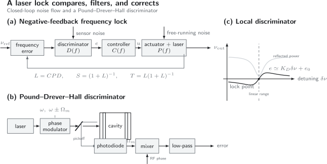
A frequency lock has three separable layers. (a) The discriminator $D$, controller $C$, and actuator–laser plant $P$ form open-loop gain $L=CPD$. (b) In a Pound–Drever–Hall discriminator, phase modulation creates a carrier and sidebands; the cavity-reflected beat at $\Omega_m$ is synchronously demodulated. (c) Near the selected zero crossing, $e\simeq K_D\delta\nu+e_0$. The slope $K_D$ converts voltage noise and offsets into equivalent frequency noise and bias.

Frequency Noise

Stabilize the quantity the experiment sees

Laser frequency can fluctuate through:

• intrinsic phase diffusion;
• pump or injection-current noise;
• cavity-length and refractive-index fluctuations;
• acoustic and seismic motion;
• thermal drift;
• optical feedback;
• actuator electronics;
• mode hops or cycle slips;
• phase noise added after the lock point by fibers and free-space paths.

The same source can be harmless in one experiment and dominant in another. A cooling transition may tolerate short-time phase noise but not a slow drift through resonance. A Ramsey sequence weights laser phase at separated pulses. A Raman transition is often sensitive to relative phase between two fields while rejecting common master-laser phase. A frequency comb transfers the residual phase noise of its beat locks and optical paths.

The proper requirement is therefore a sensitivity-weighted quantity:

$$\sigma_\Phi^2 = \int_0^\infty \left| H_\Phi(f) \right|^2 S_\phi(f)\,df,$$

or an analogous frequency-weighted integral. The experiment determines $H_\Phi(f)$. A single optical FWHM does not encode that weighting. Ramsey Interferometry develops one important example.

A local discriminator

Near a chosen lock point, a calibrated discriminator can be linearized as

$$e(f) = D(f)\,\delta\nu(f) + n_s(f),$$

where $e$ is measured error voltage and $n_s$ collects detector and electronic noise referred to the discriminator output. At low Fourier frequency one often writes

$$D(0) = K_D = \left. \frac{de}{d\nu} \right|_{\nu_{\rm lock}}.$$

The equivalent input frequency-noise PSD is

$$S_{\nu,\rm sens}(f) = \frac{ S_{e,\rm sens}(f) }{ |D(f)|^2 }.$$

A steeper slope is useful only if it is stable and if its increased optical power, modulation, or detector gain does not add comparable noise or systematic shift.

Three ranges should not be confused:

• linear range: detuning interval over which $e\simeq K_D\delta\nu$ is accurate;
• capture range: initial detuning and velocity from which the loop converges to the desired zero;
• hold range: disturbance range that available actuator travel and closed-loop dynamics can follow after acquisition.

A narrow, steep discriminator may give excellent residual noise but poor capture. Practical systems often combine a broad acquisition signal with a narrow precision signal.

Offset is frequency bias

If the discriminator has a DC offset $e_0$, the apparent zero occurs at

$$\delta\nu_{\rm bias} = - \frac{e_0}{K_D}.$$

Offsets can arise from:

• residual amplitude modulation;
• detector dark current or amplifier offset;
• mixer quadrature error;
• etalons;
• beam pointing and mode-matching changes;
• polarization drift;
• unequal optical sidebands;
• atomic background slopes;
• digital quantization or numerical bias.

Increasing feedback gain does not remove a discriminator offset. It makes the laser follow the shifted zero more faithfully.

Sensor floor and optical power

For mean photodiode current $\bar I_{\rm pd}$, ideal one-sided shot-noise current amplitude is

$$\sqrt{S_i^{(1)}} = \sqrt{2q\bar I_{\rm pd}}.$$

After a transimpedance $Z_T(f)$, this gives voltage-noise ASD

$$\sqrt{S_e^{(1)}} = |Z_T(f)| \sqrt{2q\bar I_{\rm pd}}.$$

The equivalent frequency ASD is this voltage ASD divided by $|D(f)|$. Electronics noise, laser relative-intensity noise, optical loss, detector saturation, and demodulation efficiency add to the real floor.

Raising optical power can improve shot-noise-limited slope, but it can also heat a reference cavity, increase residual amplitude modulation, saturate an atomic line, produce AC Stark shifts, and overload a detector. “More power” is not a universal stabilization strategy.

Reference Cavities

A cavity is a length-to-frequency transducer

For a simple linear reference cavity with one-way group-delay length $L_{\rm gd}$,

$$\nu_q \simeq \frac{q c}{2L_{\rm ph}}, \qquad \Delta\nu_{\rm FSR} \simeq \frac{c}{2L_{\rm gd}},$$

where $L_{\rm ph}$ sets the resonance phase and $L_{\rm gd}$ sets adjacent mode spacing. In a weakly dispersive vacuum cavity they are both close to the geometric length $L$.

For a fixed longitudinal order,

$$\frac{\delta\nu_q}{\nu_q} \simeq - \frac{\delta L_{\rm ph}}{L_{\rm ph}}.$$

A fractional length fluctuation of $10^{-15}$ is therefore a fractional frequency fluctuation of approximately $10^{-15}$. At $300\ {\rm THz}$ that is $0.3\ {\rm Hz}$.

The power linewidth is

$$\Delta\nu_{\rm cav} = \frac{\Delta\nu_{\rm FSR}}{\mathcal F},$$

with finesse $\mathcal F$. A narrower cavity resonance can provide a steeper frequency discriminator, but only while technical and thermodynamic length noise remain below the desired frequency noise.

The reference moves

A laser locked tightly to a cavity follows the cavity’s optical length. Relevant fluctuations include:

• spacer thermal expansion;
• mirror-substrate and coating Brownian motion;
• thermoelastic and thermorefractive noise;
• vibration and acceleration sensitivity;
• acoustic pressure;
• residual-gas refractive-index changes;
• support-force and mounting stress;
• optical-power-dependent coating and substrate heating;
• slow material aging and creep;
• contamination or mirror degradation.

Feedback cannot distinguish “true laser noise” from reference-cavity motion. Both appear as detuning. At high loop gain, cavity motion is deliberately transferred to the laser.

Thermal design

Ultra-low-expansion glass has a temperature where its linear thermal expansion coefficient crosses zero. Operating near that point suppresses the first-order temperature coefficient, but does not eliminate:

• curvature of the expansion law;
• gradients between shield, spacer, mirrors, and supports;
• finite thermal time constants;
• mirror-substrate expansion;
• thermorefractive response;
• Brownian noise.

Nested thermal shields in vacuum reduce air-index fluctuations, convection, and rapid environmental changes. The control sensor must represent the relevant cavity temperature rather than only the outer enclosure. Over-aggressive temperature feedback can inject sensor noise into the cavity on time scales where passive thermal filtering was quieter.

Vibration sensitivity

For small acceleration $\mathbf a$, a cavity’s fractional frequency response can be summarized locally by

$$\frac{\delta\nu}{\nu} = \mathbf k_a\cdot\mathbf a,$$

where $\mathbf k_a$ is an acceleration-sensitivity vector in $\mathrm{g^{-1}}$ or $\mathrm{(m\,s^{-2})^{-1}}$. Its value depends on spacer shape, mirror deformation, support points, orientation, and mounting force.

A vertical, horizontal, cubic, or transportable cavity is not quiet merely because of its geometry label. Sensitivity should be measured along three axes and, when relevant, for rotations. Support preload and cable forces can change it after installation.

Optical operating point

The cavity lock also depends on:

• matching the laser to the desired transverse mode;
• avoiding nearby higher-order resonances;
• stabilizing polarization;
• choosing coupling close to the intended impedance match;
• controlling incident power;
• suppressing parasitic etalons;
• preventing scattered light from returning to the laser;
• sampling the same optical path used by the experiment when path noise matters.

A high-finesse cavity has a narrow linear range. A frequency excursion can land on an adjacent longitudinal or transverse mode while a lock indicator still reports success. Transmission monitoring and coarse absolute-frequency checks are valuable state discriminators.

Transmission, polarization, and phase discriminators

Direct cavity transmission is even in detuning near resonance and does not provide a signed error without modulation or an offset operating point. Common alternatives are:

Method	Signed information	Main strength	Main vulnerability
dither lock	modulate frequency or length and demodulate transmission	simple and broad applicability	imposed frequency modulation and limited bandwidth
side-of-fringe lock	operate on a transmission slope	minimal electronics	converts intensity noise to frequency error and gives asymmetric range
Hänsch–Couillaud	analyze polarization of reflected light	modulation free	polarization drift and intracavity birefringence
Pound–Drever–Hall	phase-modulate and demodulate reflected light	steep, high-bandwidth phase discriminator	residual amplitude modulation, RF phase, etalons

Pound–Drever–Hall Overview

Phase-modulated input

Let the incident positive-frequency field be

$$E_{\rm in}^{(+)}(t) = E_0 e^{i\omega t} e^{i\beta\sin\Omega_m t},$$

where $\beta$ is phase-modulation index. The Jacobi–Anger expansion gives

$$e^{i\beta\sin\Omega_m t} = \sum_{n=-\infty}^{\infty} J_n(\beta)e^{in\Omega_m t}.$$

Keeping the carrier and first sideband pair,

$$\begin{aligned} E_{\rm in}^{(+)}(t) \simeq E_0\big[ &J_0(\beta)e^{i\omega t} \\ &+ J_1(\beta)e^{i(\omega+\Omega_m)t} \\ &- J_1(\beta)e^{i(\omega-\Omega_m)t} \big]. \end{aligned}$$

Pure phase modulation has equal first-order sideband powers and, before any dispersive element, no intensity beat at $\Omega_m$.

Complex cavity reflection

Let $r(\Delta)$ be the cavity’s complex field reflection coefficient at angular detuning $\Delta$ from the selected resonance. Define

$$\begin{aligned} r_0 &= r(\Delta), \\ r_+ &= r(\Delta+\Omega_m), \\ r_- &= r(\Delta-\Omega_m). \end{aligned}$$

The reflected field is

$$\begin{aligned} E_{\rm r}^{(+)}(t) \simeq E_0\big[ &J_0r_0e^{i\omega t} \\ &+ J_1r_+e^{i(\omega+\Omega_m)t} \\ &- J_1r_-e^{i(\omega-\Omega_m)t} \big]. \end{aligned}$$

Square-law detection produces a photocurrent component at $\Omega_m$. Up to the photodiode responsivity and optical-power normalization, its complex amplitude is

$$A_{\Omega_m} \propto J_0J_1 \left( r_0^*r_+ - r_0r_-^* \right).$$

Mixing the photocurrent with an RF local oscillator of phase $\phi_d$ and low-pass filtering selects a quadrature,

$$e_{\rm PDH} \propto \operatorname{Re} \left[ A_{\Omega_m}e^{-i\phi_d} \right].$$

The demodulation phase is chosen so the desired quadrature is odd in detuning and has maximum local slope.

Resolved-sideband operating regime

A common design regime is

$$\Delta\nu_{\rm cav} \ll f_m \ll \Delta\nu_{\rm FSR},$$

while also avoiding transverse-mode resonances. The carrier then samples the rapid complex reflection change near the chosen cavity mode, while the sidebands are approximately promptly reflected. In that limit, the demodulated signal is proportional, up to sign and scale, to the dispersive quadrature of $r_0$.

Near resonance,

$$e_{\rm PDH} \simeq K_D\,\delta\nu + e_{\rm RAM} + n_e.$$

The PDH signal is a phase-sensitive frequency discriminator, not merely the derivative of the transmitted power. Describing it only as “differentiate the cavity resonance” loses the heterodyne physics and obscures offset mechanisms.

Modulation frequency and depth

The modulation frequency should:

• place the first sidebands well outside the carrier resonance;
• avoid adjacent longitudinal and transverse modes;
• lie within EOM, photodiode, amplifier, and mixer bandwidth;
• avoid strong RF pickup or cable resonances;
• support the desired control bandwidth;
• remain compatible with any downstream experiment that sees the sidebands.

The modulation index controls carrier and sideband powers through $J_0$ and $J_1$. Maximizing the simple product $J_0J_1$ is not always optimal. Detector headroom, higher-order sidebands, RAM, available RF power, cavity coupling, and whether sidebands perturb the atoms all matter.

Residual amplitude modulation

A real phase modulator can also produce amplitude modulation because of:

• imperfect polarization alignment;
• crystal birefringence;
• parasitic etalons;
• temperature drift;
• electrode imbalance;
• beam motion;
• polarization-dependent downstream optics.

RAM produces a photocurrent at $\Omega_m$ even without the desired cavity phase response. Its demodulated component shifts the PDH zero. If its equivalent offset is $e_{\rm RAM}$,

$$\delta\nu_{\rm RAM} \simeq - \frac{e_{\rm RAM}}{K_D}.$$

RAM can be reduced by polarization control, wedged and antireflection-coated optics, EOM temperature stabilization, spatial filtering, RF adjustment, or an auxiliary RAM servo. It must be measured under realistic optical power and temperature, not inferred from component specifications.

Mode matching and prompt reflection

Light not coupled to the resonant spatial mode is promptly reflected. Ideally its pure phase modulation contributes no demodulated offset, but mode mismatch can interact with:

• RAM;
• detector clipping;
• higher-order-mode resonances;
• wavefront curvature changes;
• scattered-light paths.

Cavity transmission is therefore useful for optimizing mode matching even though reflection provides the PDH error. Alignment drift can change $K_D$ and offset without visibly changing the controller settings.

Cavity dynamics are part of the discriminator

The cavity power FWHM and stored-energy lifetime obey

$$\Delta\nu_{\rm cav} = \frac{1}{2\pi\tau_p}$$

under the present convention. The ordinary field-response pole is then of order

$$f_{\rm pole} \simeq \frac{\Delta\nu_{\rm cav}}{2}.$$

The complete PDH response to laser phase or frequency modulation is more subtle than one scalar low-pass pole, especially above the cavity bandwidth. The reflected prompt field and leaked intracavity field interfere, and the detector, RF chain, cables, and actuator add their own phase. High-bandwidth design should use a measured transfer function rather than assuming a static $K_D$ at every Fourier frequency.

Atomic References

A transition is not an unperturbed number in the laboratory

An atomic or molecular resonance ties the laser to an internal energy difference. It can provide long-term reproducibility and an absolute physical meaning that an isolated spacer cavity lacks. The observed lock point, however, can shift with:

• magnetic fields and polarization;
• electric fields and AC Stark shifts;
• optical power and saturation;
• gas pressure and buffer-gas composition;
• cell temperature and density;
• collisions and wall interactions;
• pump–probe angle and wavefront;
• unresolved neighboring transitions;
• crossover resonances;
• modulation depth and demodulation phase;
• etalon backgrounds and detector offsets.

An atomic lock is only as absolute as its line assignment, environmental control, and shift budget. Precision Spectroscopy develops that budget in detail.

Common vapor-cell discriminators

Method	Signal mechanism	Useful property	Main caution
saturated absorption	counterpropagating pump and probe select a narrow velocity class	simple sub-Doppler features	crossover resonances, background slope, power and alignment shifts
polarization spectroscopy	pump-induced circular birefringence gives a dispersive probe signal	modulation free and naturally signed	polarization and magnetic sensitivity
modulation-transfer spectroscopy	nonlinear medium transfers pump modulation to probe	background-free dispersive features near closed transitions	more demanding alignment and RF optimization
DAVLL	magnetic-field-induced circular dichroism gives a broad dispersive signal	large capture range and robust relocking	field, temperature, polarization, and broad-feature offsets
frequency-modulation spectroscopy	phase/frequency modulation and heterodyne detection measure dispersion or absorption	high sensitivity and flexible bandwidth	RAM and demodulation offsets

A two-stage lock can use a broad DAVLL-like signal for acquisition and a narrow sub-Doppler feature for precision. The handoff logic must prevent the controller from selecting the wrong isotope, hyperfine line, or crossover.

Generate a signed atomic error

If a measured spectroscopic signal $A(\nu)$ is locally symmetric, a small frequency dither

$$\nu_L(t) = \bar\nu_L + \delta\nu_m\cos\Omega_m t$$

produces, to first order,

$$A(t) \simeq A(\bar\nu_L) + \left. \frac{dA}{d\nu} \right|_{\bar\nu_L} \delta\nu_m\cos\Omega_m t.$$

Synchronous demodulation therefore yields a derivative-like signal. The approximation requires modulation depth small compared with the spectral scale of interest. Large modulation changes the line shape and can shift the zero through asymmetry.

Polarization and modulation-transfer methods can produce dispersive signals without a simple frequency dither of the detected beam, but they still require calibration of slope, offset, and environmental dependence.

Offset and transfer locks

The experiment may need a stable frequency displaced from the available reference. Options include:

• place an AOM between the locked source and experiment;
• lock an EOM sideband to the reference;
• phase-lock a second laser to an optical beat;
• lock a transfer cavity to one laser and another laser to a different cavity mode;
• use an optical frequency comb to compare or synthesize widely separated frequencies.

An AOM offset is set by its RF source but can add path, pointing, and diffraction-efficiency noise. A transfer cavity maps its own length and dispersion noise into the second wavelength. A beat lock requires correct beat sign, adequate signal-to-noise ratio, and cycle-slip detection. Frequency Combs owns the comb-coordinate and transfer-oscillator details.

Hybrid short- and long-term references

A quiet cavity often gives the best short-time coherence, while an atom, molecule, or primary standard gives better long-time meaning. A hybrid system can:

1. lock the laser rapidly to the cavity;
2. measure cavity drift against an atomic line or comb;
3. steer cavity temperature, an AOM offset, or a slow frequency command;
4. keep the fast loop unaware of the slow reference except through a bounded set point.

The two loops must be separated in bandwidth and sign. Otherwise they can fight, amplify sensor noise near the crossover, or drive an actuator to its rail.

Feedback Loops

Closed-loop derivation

Let the laser output be

$$\nu_L = \nu_{\rm free} + P \left( u+n_u \right),$$

where $n_u$ is actuator-drive noise added after the controller. Let

$$\begin{aligned} e &= D \left( \nu_L-\nu_{\rm ref} \right) + n_s, \\ u &= - C e. \end{aligned}$$

All quantities are functions of Fourier frequency $f$. Substitution gives

$$\begin{aligned} \left( 1+CPD \right)\nu_L ={}& \nu_{\rm free} + CPD\,\nu_{\rm ref} \\ &+ P n_u - CP n_s. \end{aligned}$$

With

$$L=CPD, \qquad S=\frac{1}{1+L}, \qquad T=\frac{L}{1+L},$$

and equivalent sensor frequency noise $n_{\nu,s}=n_s/D$,

$$\nu_L = S\nu_{\rm free} + T\nu_{\rm ref} + PS n_u - T n_{\nu,s}.$$

This equation is the central noise ledger:

• where $|L|\gg1$, $S\to0$ and $T\to1$: free-running laser noise is suppressed, but reference and sensor noise are transferred;
• where $|L|\ll1$, $S\to1$ and $T\to0$: the laser is nearly free running;
• actuator noise is filtered by $PS$, with its exact effect depending on where it enters the plant.

For mutually uncorrelated sources,

$$\begin{aligned} S_{\nu,L}(f) \simeq{}& |S|^2S_{\nu,\rm free} + |T|^2S_{\nu,\rm ref} \\ &+ |PS|^2S_u + |T|^2S_{\nu,\rm sens}. \end{aligned}$$

Correlated paths require cross-spectral terms. Treating a shared oscillator, shared optical path, or common power fluctuation as independent can overestimate or underestimate residual noise.

Why the in-loop error can lie

Using the same equations,

$$e = D S \left( \nu_{\rm free}-\nu_{\rm ref}+Pn_u \right) + S n_s.$$

At high gain, the measured in-loop contribution from $n_s$ is suppressed by $S$. Yet the laser output contains approximately $-n_s/D$ through the $-Tn_{\nu,s}$ term. The loop has squashed the detector noise in its own readout by moving the laser.

Therefore an in-loop spectrum demonstrates loop operation but cannot alone establish residual optical noise. A second independent discriminator, optical beat, second cavity, atomic signal, or path endpoint provides an out-of-loop test.

Gain and phase margins

Negative feedback becomes positive when accumulated phase reaches $-180^\circ$ while loop magnitude remains at least unity. Define the gain-crossover frequency $f_u$ by

$$|L(f_u)| = 1.$$

The phase margin is

$$\phi_m = 180^\circ + \arg L(f_u).$$

Small positive margin gives ringing and a servo bump; negative margin gives instability. Gain margin asks how much loop magnitude can increase at the $-180^\circ$ phase crossing before instability.

A pure delay contributes

$$\arg L_{\rm delay} = - 2\pi f\tau,$$

or

$$\phi_{\rm delay} = - 360^\circ f\tau.$$

One microsecond already contributes $-36^\circ$ at $100\ {\rm kHz}$. Photodiode response, filters, ADC and DAC latency, computation, cables, actuator resonances, and the optical reference all consume phase margin.

Loop shaping

Common controller elements have distinct jobs:

• an integrator gives large low-frequency gain and zero steady error to a constant disturbance;
• a proportional path raises midband gain;
• a lead network adds phase near crossover;
• a lag network increases lower-frequency gain at the cost of phase;
• a notch reduces gain at a narrow actuator resonance;
• a low-pass roll-off limits high-frequency noise injection and protects stability.

More integrators do not automatically make a better lock. Each ideal integrator contributes $-90^\circ$. Real plants add poles and delays. Controller design should start from a measured complex plant and discriminator transfer function, not only a fitted time-domain step.

A useful workflow is:

1. measure actuator response $P(f)$ at the actual laser operating point;
2. measure discriminator response $D(f)$, including cavity and RF phase;
3. set low-frequency gain from the drift requirement;
4. choose crossover below poorly controlled resonances and delays;
5. add lead or notches with explicit margin targets;
6. close the loop at low gain and verify sign;
7. measure closed-loop suppression and the open-loop return ratio;
8. check output noise out of loop.

Servo bump

Near unity gain, $|S|$ or $|T|$ can exceed one if phase margin is limited. Noise is then amplified in a servo bump. That bump may dominate an experiment even while the low-frequency error is excellent.

For pulsed coherent control, compare the bump with the pulse-sequence sensitivity function. Moving it to higher Fourier frequency is useful only if the experiment and actuator do not remain sensitive there.

Multiple actuators

No practical laser actuator has unlimited range and bandwidth. Semiconductor Lasers Overview details current, temperature, and external-cavity tuning. A common allocation is:

Band	Actuator	Strength	Failure mode
fast	injection current, intracavity EOM, or external frequency actuator	high bandwidth	small range, amplitude coupling, resonances
intermediate	cavity or grating piezo	useful range with moderate bandwidth	mechanical resonances, hysteresis
slow	temperature or motor	large range and drift removal	delay, overshoot, thermal cross-coupling

An offload loop monitors the fast actuator’s mean command and transfers its DC burden to a slower actuator. Anti-windup prevents an integrator from continuing to charge while an actuator is saturated. Crossovers should be designed so two actuators cooperate rather than issue opposite commands with similar gain.

Digital implementation

Digital controllers add:

• sampling and zero-order-hold response;
• ADC and DAC latency;
• computation delay;
• quantization and finite word length;
• aliasing;
• clock phase noise;
• numerical saturation and wraparound.

The sampling rate must exceed the control bandwidth with enough margin for anti-alias filters and phase delay. A fast nominal sample rate does not remove latency from buffering, bus transfers, or block processing. Transfer functions should be measured through the complete deployed signal path.

Acquisition and relocking

A precision discriminator usually has several zero crossings and a limited capture range. Robust automation separates acquisition from hold:

1. scan or coarsely tune while monitoring a broad marker;
2. identify the desired cavity mode or atomic feature;
3. place actuators away from their rails;
4. enable the precision loop with bounded gain;
5. ramp to the operating controller;
6. verify transmission, side-mode, beat, or atomic-state conditions;
7. declare lock only after a dwell-time test;
8. on failure, open the loop, reset integrators, and restart safely.

A zero error voltage is not sufficient state identification. The beam may be blocked, the detector saturated, the laser on a neighboring mode, or the controller railed.

Feedforward and disturbance cancellation

If a disturbance is measured before it reaches the laser, feedforward can cancel it without waiting for an error. Examples include:

• acceleration feedforward to a transportable cavity;
• current feedforward during a piezo frequency scan;
• AOM-frequency correction for a known chirp;
• path-phase correction from an interferometric monitor.

Feedforward depends on a model and calibration. It does not correct unmeasured disturbances, and an incorrect phase can add noise. Feedback remains necessary for model error and drift.

Choosing and Validating a Lock

Reference comparison

Reference	Short-term potential	Long-term meaning	Main limitation
passive cavity	excellent phase discrimination	follows cavity drift	thermal, vibration, and Brownian length noise
vapor-cell line	moderate to good	tied to a named transition	pressure, power, field, line-shape, and cell shifts
trapped atom or ion	excellent when fully realized	high accuracy	complex state preparation and intermittent interrogation
another laser	relative coherence	inherits reference laser	requires independent knowledge of reference
delay line	broad frequency-noise discrimination	delay itself is not absolute	path-length noise and periodic response
frequency comb	coherent transfer over wide spectral span	inherits clock or optical reference	beat SNR, path noise, and cycle slips

The “best” reference is the one whose noise and drift are below the experiment’s requirement in the relevant band and whose systematic shifts can be controlled.

Reporting checklist

A reproducible stabilization result should state:

1. laser type, wavelength, optical power, and operating point;
2. reference type and environmental controls;
3. discriminator method, modulation frequency and depth, and calibrated $D(f)$;
4. actuator transfer functions and command ranges;
5. controller transfer function or enough information to reconstruct it;
6. unity-gain frequency, phase margin, and important resonances;
7. in-loop and out-of-loop measurement methods;
8. Fourier-frequency span, PSD convention, resolution, and record duration;
9. drift removal, dead time, and mode-hop or cycle-slip treatment;
10. residual amplitude modulation and offset evaluation;
11. stability, accuracy, lock uptime, and relock criteria;
12. where in the optical path the result was measured.

“Stable enough” is a quantitative claim

For an experiment, close the chain:

$$\text{source noise} \longrightarrow \text{closed-loop residual} \longrightarrow \text{delivered-path noise} \longrightarrow \text{experimental sensitivity} \longrightarrow \text{observable error}.$$

That final observable may be cooling temperature, excitation probability, Rabi contrast, Ramsey phase, clock instability, or a spectroscopic line-center uncertainty. A quieter in-loop trace is useful only if it reduces the relevant observable.

Worked Example: A Closed-Loop Noise Point

At $f=1\ {\rm kHz}$, suppose the open-loop gain is real and positive with

$$L=99,$$

so

$$S=\frac{1}{100}=0.010, \qquad T=\frac{99}{100}=0.990.$$

Let the free-running laser frequency-noise ASD be $10^4\ {\rm Hz/\sqrt{Hz}}$, the reference ASD be $20\ {\rm Hz/\sqrt{Hz}}$, and equivalent sensor ASD be $10\ {\rm Hz/\sqrt{Hz}}$. Neglect actuator noise and correlations.

The residual ASD is the quadrature sum

$$\begin{aligned} \sqrt{S_{\nu,L}} ={}& \left[ |S|^2 \left( 10^4 \right)^2 \right. \\ &\left. + |T|^2 \left( 20^2+10^2 \right) \right]^{1/2} \\ \simeq{}& 102.4\ {\rm Hz/\sqrt{Hz}}. \end{aligned}$$

The free-running contribution has fallen to $100\ {\rm Hz/\sqrt{Hz}}$, but it still dominates slightly. Infinite gain would not make the result zero; it would approach the combined reference and sensor floor,

$$\sqrt{20^2+10^2} \simeq 22.4\ {\rm Hz/\sqrt{Hz}}.$$

Common Mistakes

1. Treating a lock as noise erasure. High gain replaces free-running laser noise with reference and sensor noise.
2. Using a symmetric transmission peak as a signed error. A stable lock needs a local direction as well as a magnitude.
3. Quoting a slope without units or bandwidth. $D(f)$ can have amplitude and phase dependence; a DC slope is not a broadband transfer function.
4. Ignoring offsets. Feedback follows the discriminator zero, including RAM, etalon, detector, and spectroscopy biases.
5. Reading the in-loop floor as optical noise. Noise squashing can make the sensor quiet while its noise is imposed on the laser.
6. Setting PDH modulation frequency from cavity linewidth alone. Adjacent longitudinal and transverse modes and RF hardware also constrain it.
7. Calling PDH the derivative of transmission. It is a reflected-field heterodyne phase measurement.
8. Assuming a cavity resonance is an absolute reference. Its optical length drifts and fluctuates.
9. Calling an atomic feature unshifted. Power, pressure, magnetic field, polarization, and line pulling move laboratory zero crossings.
10. Raising gain until oscillation and backing off slightly. This gives an undocumented and usually fragile phase margin.
11. Ignoring actuator saturation and windup. A linear loop model no longer applies at the rail.
12. Letting fast and slow loops fight. Actuator handoff needs explicit crossover and offload logic.
13. Designing from a static tuning coefficient. Current, piezo, cavity, and electronics responses are frequency dependent and can change sign.
14. Validating at the laser head only. Fiber, AOM, free-space, and reference-path noise can be added after the lock.

Exercises

1. Equivalent discriminator noise

A discriminator has low-frequency slope $K_D=4.0\ {\rm mV\,kHz^{-1}}$. Its output electronics have white voltage-noise ASD $12\ {\rm nV/\sqrt{Hz}}$. Find the equivalent frequency-noise ASD.

Solution

Convert the slope:

$$K_D = 4.0\times10^{-6}\ {\rm V\,Hz^{-1}}.$$

Then

$$\begin{aligned} \sqrt{S_{\nu,\rm sens}} &= \frac{ 12\times10^{-9}\ {\rm V/\sqrt{Hz}} }{ 4.0\times10^{-6}\ {\rm V/Hz} } \\ &= 3.0\times10^{-3}\ {\rm Hz/\sqrt{Hz}}. \end{aligned}$$

This is only the electronics contribution. Optical shot noise, intensity noise, and slope fluctuations must be added.

2. Cavity length requirement

A laser at $282\ {\rm THz}$ is locked to a $10.0\ {\rm cm}$ vacuum cavity. What cavity-length change produces a $1.0\ {\rm Hz}$ frequency shift?

Solution

Use

$$\frac{\delta\nu}{\nu} = - \frac{\delta L}{L}.$$

Therefore

$$\begin{aligned} \delta L &= - L\frac{\delta\nu}{\nu} \\ &= - (0.100\ {\rm m}) \frac{ 1.0\ {\rm Hz} }{ 282\times10^{12}\ {\rm Hz} } \\ &\simeq - 3.55\times10^{-16}\ {\rm m}. \end{aligned}$$

The sub-femtometer scale explains why thermal, elastic, and vibration design are central to cavity-stabilized lasers.

3. Cavity linewidth and pole

A $10.0\ {\rm cm}$ vacuum cavity has finesse $\mathcal F=3.0\times10^5$. Estimate its FSR, power FWHM, stored-energy lifetime, and ordinary field-response pole under this page’s conventions.

Solution

The FSR is

$$\Delta\nu_{\rm FSR} = \frac{c}{2L} \simeq 1.499\ {\rm GHz}.$$

The power linewidth is

$$\Delta\nu_{\rm cav} = \frac{ 1.499\times10^9 }{ 3.0\times10^5 } \simeq 5.00\ {\rm kHz}.$$

From $\Delta\nu_{\rm cav}=1/(2\pi\tau_p)$,

$$\tau_p \simeq \frac{1}{ 2\pi(5.00\times10^3) } \simeq 31.8\ \mu{\rm s}.$$

The ordinary field-response pole scale is

$$f_{\rm pole} \simeq \frac{\Delta\nu_{\rm cav}}{2} \simeq 2.50\ {\rm kHz}.$$

A full PDH loop model must still include prompt reflection and the rest of the RF and actuator chain.

4. Check a PDH modulation frequency

For the cavity in Exercise 3, a proposed PDH modulation frequency is $f_m=20\ {\rm MHz}$. Check the basic longitudinal-mode inequalities and state two additional checks.

Solution

The hierarchy is

$$5.00\ {\rm kHz} \ll 20\ {\rm MHz} \ll 1.499\ {\rm GHz},$$

so the first sidebands are far outside the carrier resonance and far from adjacent longitudinal modes.

One must also verify that the sidebands do not overlap a transverse-mode resonance and that the EOM, photodiode, RF amplifier, mixer, cables, and local oscillator have suitable response at $20\ {\rm MHz}$. RAM and downstream atomic sensitivity to the sidebands should also be checked.

5. Offset-to-frequency conversion

A PDH discriminator has $K_D=2.0\ {\rm mV\,kHz^{-1}}$. A RAM drift changes the demodulated offset by $+0.60\ {\rm mV}$. Find the locked-frequency shift under the sign convention $e=K_D\delta\nu+e_{\rm RAM}$.

Solution

The loop drives the measured error to zero:

$$0 = K_D\delta\nu + e_{\rm RAM}.$$

Thus

$$\begin{aligned} \delta\nu &= - \frac{ 0.60\ {\rm mV} }{ 2.0\ {\rm mV\,kHz^{-1}} } \\ &= - 0.30\ {\rm kHz} \\ &= - 300\ {\rm Hz}. \end{aligned}$$

Higher loop gain makes the laser approach this biased zero more closely; it does not remove the $300\ {\rm Hz}$ shift.

6. Closed-loop noise budget

At one Fourier frequency, let $|L|=49$ with negligible phase, free-running laser ASD $500\ {\rm Hz/\sqrt{Hz}}$, reference ASD $4.0\ {\rm Hz/\sqrt{Hz}}$, and equivalent sensor ASD $3.0\ {\rm Hz/\sqrt{Hz}}$. Neglect actuator noise and correlations. Find the closed-loop ASD.

Solution

Here

$$S = \frac{1}{50} = 0.020, \qquad T = \frac{49}{50} = 0.980.$$

The uncorrelated residual is

$$\begin{aligned} \sqrt{S_{\nu,L}} &= \left[ (0.020)^2(500)^2 \right. \\ &\qquad\left. + (0.980)^2 \left( 4.0^2+3.0^2 \right) \right]^{1/2} \\ &\simeq 11.1\ {\rm Hz/\sqrt{Hz}}. \end{aligned}$$

The free-running contribution is $10.0\ {\rm Hz/\sqrt{Hz}}$ and the combined transferred reference–sensor contribution is $0.98\sqrt{4^2+3^2}=4.9\ {\rm Hz/\sqrt{Hz}}$.

7. Delay and phase margin

At a proposed unity-gain frequency $f_u=100\ {\rm kHz}$, the controller, actuator, and discriminator excluding pure delay contribute $-120^\circ$. The total loop delay is $1.0\ \mu{\rm s}$. Find the delay phase and phase margin. Repeat at $200\ {\rm kHz}$ if the non-delay phase remains $-120^\circ$.

Solution

At $100\ {\rm kHz}$,

$$\phi_{\rm delay} = - 360^\circ (100\times10^3) (1.0\times10^{-6}) = - 36^\circ.$$

The total phase is $-156^\circ$, so

$$\phi_m = 180^\circ-156^\circ = 24^\circ.$$

That positive but small margin is likely to give a pronounced servo bump.

At $200\ {\rm kHz}$, the delay contributes $-72^\circ$. The total phase is $-192^\circ$, giving nominal margin

$$\phi_m = - 12^\circ.$$

Unity gain there would be unstable under the stated model.

8. Design a hybrid lock

An experiment needs sub-kilohertz short-time coherence and long-term reproducibility to an atomic transition. A high-finesse cavity is quiet above $0.1\ {\rm Hz}$ but drifts by several kilohertz per hour. An atomic discriminator is reproducible at long times but too noisy above $1\ {\rm Hz}$. Propose a loop hierarchy and validation measurements.

Solution

A suitable architecture is:

1. lock the laser rapidly to the cavity with PDH using fast and intermediate actuators;
2. measure the cavity-locked laser against the atomic discriminator or a comb referenced to the atomic standard;
3. low-pass that long-term error with crossover well below $0.1\ {\rm Hz}$;
4. steer an AOM offset, cavity temperature set point, or slow laser set point so the cavity-locked output tracks the atomic reference only at long times;
5. use anti-windup and limit the slow correction rate so it does not enter the fast coherence band.

Validation should include an out-of-loop optical beat or second cavity for short-time phase noise, an independent atomic measurement for long-time accuracy, logged actuator ranges, RAM monitoring, and a test for mode hops or cycle slips. The crossover should be checked in both PSD and Allan-deviation representations.

References

1. R. V. Pound, “Electronic Frequency Stabilization of Microwave Oscillators”, Review of Scientific Instruments 17, 490–505 (1946). Foundational cavity-discriminator and heterodyne frequency stabilization.
2. C. Wieman and T. W. Hänsch, “Doppler-Free Laser Polarization Spectroscopy”, Physical Review Letters 36, 1170–1173 (1976).
3. T. W. Hänsch and B. Couillaud, “Laser Frequency Stabilization by Polarization Spectroscopy of a Reflecting Reference Cavity”, Optics Communications 35, 441–444 (1980).
4. J. H. Shirley, “Modulation Transfer Processes in Optical Heterodyne Saturation Spectroscopy”, Optics Letters 7, 537–539 (1982).
5. R. W. P. Drever, J. L. Hall, F. V. Kowalski, J. Hough, G. M. Ford, A. J. Munley, and H. Ward, “Laser Phase and Frequency Stabilization Using an Optical Resonator”, Applied Physics B 31, 97–105 (1983). Foundational optical PDH treatment.
6. C. E. Wieman and L. Hollberg, “Using Diode Lasers for Atomic Physics”, Review of Scientific Instruments 62, 1–20 (1991). Diode-laser control and atomic-reference practice.
7. K. L. Corwin, Z.-T. Lu, C. F. Hand, R. J. Epstein, and C. E. Wieman, “Frequency-Stabilized Diode Laser with the Zeeman Shift in an Atomic Vapor”, Applied Optics 37, 3295–3298 (1998). The dichroic atomic vapor laser lock.
8. E. D. Black, “An Introduction to Pound–Drever–Hall Laser Frequency Stabilization”, American Journal of Physics 69, 79–87 (2001). Accessible quantitative PDH derivation.
9. K. Numata, A. Kemery, and J. Camp, “Thermal-Noise Limit in the Frequency Stabilization of Lasers with Rigid Cavities”, Physical Review Letters 93, 250602 (2004).
10. M. Notcutt, L.-S. Ma, A. D. Ludlow, S. M. Foreman, J. Ye, and J. L. Hall, “Contribution of Thermal Noise to Frequency Stability of Rigid Optical Cavity via Hertz-Linewidth Lasers”, Physical Review A 73, 031804(R) (2006).
11. D. W. Allan, “Statistics of Atomic Frequency Standards”, Proceedings of the IEEE 54, 221–230 (1966). Foundational oscillator-stability statistic.
12. A. D. Ludlow, M. M. Boyd, J. Ye, E. Peik, and P. O. Schmidt, “Optical Atomic Clocks”, Reviews of Modern Physics 87, 637–701 (2015). Laser, cavity, atomic-reference, and clock stability context.
13. K. J. Åström and R. M. Murray, Feedback Systems: An Introduction for Scientists and Engineers, 2nd ed., Princeton University Press (2021). Sensitivity functions, loop shaping, margins, and nonlinear limitations.
14. F. Riehle, Frequency Standards: Basics and Applications, Wiley-VCH (2004). Optical references, stabilization, and frequency metrology.
15. A. E. Siegman, Lasers, University Science Books (1986). Cavity resonance, oscillator noise, and laser-control foundations.
16. J. L. Hall, “Nobel Lecture: Defining and Measuring Optical Frequencies”, Reviews of Modern Physics 78, 1279–1295 (2006). Precision optical-frequency control and measurement.

Further Connections

• Lasers Overview
• Optical Cavities
• Linewidth and Coherence
• Semiconductor Lasers Overview
• Frequency Combs
• Precision Spectroscopy
• Atomic Clocks
• Optical Clocks
• Frequency Standards
• Line Shapes and Broadening
• Ramsey Interferometry
• Noise Spectra