Rate-Equation Lasers

A laser is a feedback oscillator with at least two stores of energy: excitation in the gain medium and photons in a resonator mode. Laser rate equations replace the microscopic atoms and field by the mean populations of those stores. They are the first model that can describe turn-on, gain clamping, small-signal modulation, and relaxation oscillations in one calculation.

For an effective four-level, single-mode laser, the minimal equations are

$$\begin{aligned} \frac{dN}{dt} &= R - \gamma_N N - G(N)n, \\ \frac{dn}{dt} &= \left[ G(N)-\kappa \right]n + \beta\gamma_N N. \end{aligned}$$

Here $N$ is the number of reservoir excitations available to the lasing transition, $n$ is the mean intracavity photon number, $R$ is the effective pump rate, $G(N)$ is the stimulated-emission rate per photon, $\gamma_N$ is the reservoir decay rate, $\kappa$ is the cavity energy-decay rate, and $\beta$ is the fraction of reservoir decays that feed the selected mode.

These compact equations are not universal laws. They are a controlled coarse-graining with a convention ledger, a range of validity, and clear failure modes.

Canonical Scope

This page owns:

1. the event-counting derivation of a single-mode population–photon model;
2. the effective four-level approximation and its relation to level-resolved rate equations;
3. normalization to pump, inversion, and photon scales;
4. below-threshold and above-threshold fixed points;
5. gain clamping and linear output above threshold;
6. finite-$\beta$ smoothing of the deterministic input–output curve;
7. linear stability and the relaxation-oscillation frequency;
8. turn-on delay, damped spiking, and small-signal modulation;
9. the class-A, class-B, and class-C time-scale hierarchy;
10. extensions needed for semiconductor, multimode, spatial, or quantum-noise problems.

Population Inversion owns three- and four-level pumping cycles. Gain and Threshold owns modal overlap, distributed and lumped losses, and the exact round-trip threshold condition. Stimulated Emission owns microscopic cross sections and saturation. This page begins after those quantities have been reduced to effective rates. Laser Modes replaces the one-mode reduction by spatially resolved modal families and a cross-saturation matrix.

The equations below predict mean populations. They do not, by themselves, predict phase diffusion, a laser linewidth, or a photon-counting distribution. Those require Langevin sources, a master equation, or another stochastic description. Linewidth and Coherence develops the phase-noise problem after the mean operating point has been fixed.

Approximation Ledger

The minimal model assumes:

Assumption	Reduction	Warning sign
one selected cavity mode	one photon number $n(t)$	mode hopping, multiple peaks, antiphase modes
uniform effective reservoir	one population $N(t)$	pump gradients, standing-wave hole burning
fast optical polarization	eliminate atomic coherence	coherent transients or Rabi flopping
fast lower-level emptying	use an effective four-level reservoir	reabsorption or bottlenecked lower state
Markovian pump and decay	constant rates $R$, $\gamma_N$, and $\kappa$	colored noise, delayed feedback
mean-field factorization	replace correlations by products	few emitters or strong field–matter correlations
fixed mode and cavity	constant $G(N)$ and $\kappa$	thermal lensing, index drift, moving boundaries

Rate equations can still be useful when an assumption is only approximate, but fitted parameters must then be identified as effective rather than microscopic.

Convention Ledger

We use:

• $N$: total effective reservoir population, dimensionless as a count;
• $n$: mean photon number in one complete cavity mode;
• $R$: absorbed pump events transferred into that reservoir per second;
• $\gamma_N=1/\tau_N$: total reservoir decay rate;
• $\kappa=1/\tau_p$: stored-energy decay rate of the cavity mode;
• $\kappa_j$: decay rate through channel $j$, with $\kappa=\sum_j\kappa_j$;
• $G(N)$: stimulated-emission rate per cavity photon;
• $\beta$: effective fraction of reservoir decay events that place a photon in the selected mode.

The associated output photon flux through a monitored port is

$$\Phi_{\mathrm{out}} = \kappa_{\mathrm{out}}n,$$

and its optical power is

$$P_{\mathrm{out}} = \hbar\omega_\ell \kappa_{\mathrm{out}}n.$$

Some laser texts use $\kappa$ for field-amplitude decay, so photon number decays at $2\kappa$. Here the defining cold-cavity equation is

$$\left. \frac{dn}{dt} \right|_{\mathrm{cavity}} = -\kappa n.$$

Translate that definition before comparing formulas. Optical Cavities derives $\kappa$ from round-trip survival, ringdown, linewidth, finesse, and quality factor; the present page treats it as an input parameter.

Population Rate Equations

Start from level populations

Let $N_i$ be the population of atomic, molecular, or electronic level $i$. A level-resolved rate equation has the general balance form

$$\frac{dN_i}{dt} = \sum_{j\ne i} \left( W_{j\to i}N_j - W_{i\to j}N_i \right) + R_i.$$

Each term names an event:

• pumping into or out of the level;
• radiative decay;
• nonradiative decay;
• collisional transfer;
• stimulated absorption or emission.

Population is conserved when every internal transfer appears once with each sign. Only pumps, extraction, and losses to reservoirs change the total population represented by the model.

For a lasing pair with degeneracies $g_u$ and $g_l$, the gain depends on the weighted inversion

$$\Delta N = N_u - \frac{g_u}{g_l}N_l,$$

not on $N_u$ alone. The Population Inversion page develops that distinction and explains why a three-level system pays a large ground-state-depletion cost.

Effective four-level reduction

In an ideal four-level cycle:

1. the pump rapidly transfers population into the upper lasing level;
2. the lower lasing level empties much faster than the upper level;
3. reabsorption from the lower level is negligible.

Then $N_l\simeq0$, and one variable $N\simeq N_u$ represents the available gain reservoir. Before coupling it to a selected cavity mode,

$$\frac{dN}{dt} = R - \gamma_N N.$$

The no-field steady population is therefore

$$N_0 = \frac{R}{\gamma_N}.$$

Stimulated emission removes one effective reservoir excitation for each photon it adds to the mode. If one photon stimulates emission at rate $G(N)$, then $n$ photons deplete the reservoir at rate $G(N)n$:

$$\frac{dN}{dt} = R - \gamma_N N - G(N)n.$$

Near transparency, a common linear constitutive law is

$$G(N) = g \left( N-N_{\mathrm{tr}} \right),$$

where $g$ is a differential rate coefficient and $N_{\mathrm{tr}}$ is a transparency population. The ideal four-level limit sets $N_{\mathrm{tr}}=0$, giving $G(N)=gN$.

The symbol $g$ here is not a propagation gain coefficient in $\mathrm{m}^{-1}$. If $g_{\mathrm{modal}}$ is a modal power-gain coefficient and $v_g$ is group velocity, their rate-equation combination is

$$G(N) \longleftrightarrow v_g g_{\mathrm{modal}}(N).$$

Photon-Number Rate Equation

Three processes change the selected-mode photon number:

1. stimulated emission adds photons at $G(N)n$;
2. cavity loss removes photons at $\kappa n$;
3. spontaneous emission feeds the mode at $\beta\gamma_NN$.

Thus

$$\frac{dn}{dt} = G(N)n - \kappa n + \beta\gamma_N N.$$

Combining the material and field ledgers gives

$$\begin{aligned} \dot N &= R-\gamma_NN-G(N)n, \\ \dot n &= \left[ G(N)-\kappa \right]n + \beta\gamma_NN. \end{aligned}$$

The stimulated term has opposite signs in the two equations. That sign pair is an energy-accounting check: one stimulated transition removes one reservoir excitation and creates one cavity photon.

The pump and laser photon energies need not be equal. Number balance gives the event rates; energy efficiency also includes the quantum-defect factor $\omega_\ell/\omega_p$ and all pump-transfer efficiencies.

What β contains

In the minimal equations, $\beta\gamma_NN$ is shorthand. A more explicit model writes

$$R_{\mathrm{sp,mode}} = \beta_{\mathrm{sp}} \gamma_{\mathrm r}N,$$

where $\gamma_{\mathrm r}$ is radiative decay and $\beta_{\mathrm{sp}}$ is the fraction of that radiation entering the selected mode. The compact parameter is then

$$\beta = \beta_{\mathrm{sp}} \frac{\gamma_{\mathrm r}}{\gamma_N}.$$

Nonradiative decay lowers this effective $\beta$. Multimode cavities require one $\beta_\mu$ for each mode, with no reason for their sum to equal one if unmodeled radiation channels remain.

Normalize the Model

Take the ideal four-level law $G(N)=gN$. Define the threshold reservoir, threshold pump, and saturation photon scale by

$$\begin{aligned} N_{\mathrm{th}} &= \frac{\kappa}{g}, \\ R_{\mathrm{th}} &= \gamma_N N_{\mathrm{th}}, \\ n_s &= \frac{\gamma_N}{g}. \end{aligned}$$

Introduce dimensionless variables

$$x = \frac{N}{N_{\mathrm{th}}}, \qquad s = \frac{n}{n_s}, \qquad p = \frac{R}{R_{\mathrm{th}}}.$$

The equations become

$$\begin{aligned} \dot x &= \gamma_N \left( p-x-xs \right), \\ \dot s &= \kappa \left[ (x-1)s + \beta x \right]. \end{aligned}$$

This normalization exposes the physics:

• $x=1$ is the gain-equals-loss condition;
• $p=1$ is the low-$\beta$ threshold pump;
• $s$ measures photons in units of the saturation scale;
• $\kappa/\gamma_N$ controls the separation of optical and reservoir time scales.

The nullclines are

$$x = \frac{p}{1+s}$$

from $\dot x=0$, and

$$x = \frac{s}{s+\beta}$$

from $\dot s=0$. Their intersection gives the physical steady state.

Threshold Behavior

The low-β limit

First set $\beta=0$. The normalized photon equation factors:

$$\dot s = \kappa(x-1)s.$$

There are two steady branches.

For $p<1$,

$$x_* = p, \qquad s_* = 0.$$

The material follows the pump, while the selected coherent mode has no macroscopic mean population in this deterministic limit.

For $p>1$,

$$x_* = 1, \qquad s_* = p-1.$$

The reservoir is clamped at threshold and every additional effective pump event is balanced by stimulated emission and cavity loss.

The below-threshold Jacobian has eigenvalues

$$\lambda_N = -\gamma_N, \qquad \lambda_s = \kappa(p-1).$$

At $p=1$, $\lambda_s$ changes sign. The nonlasing fixed point loses stability exactly when the small-signal modal gain reaches the cavity loss.

Finite spontaneous-emission coupling

For $\beta>0$, spontaneous emission seeds the selected mode at every pump. Combining the two steady-state nullclines gives

$$p = \frac{ s(1+s) }{ s+\beta }.$$

The physical root is

$$s_* = \frac{1}{2} \left[ p-1 + \sqrt{ (p-1)^2+4\beta p } \right].$$

The reservoir follows from either

$$x_* = \frac{p}{1+s_*} = \frac{s_*}{s_*+\beta}.$$

At the conventional pump scale $p=1$,

$$s_* = \sqrt{\beta}, \qquad x_* = \frac{1}{ 1+\sqrt{\beta} }.$$

Finite $\beta$ rounds the mean input–output kink. For $\beta=1$, this minimal model gives $s_*=p$ and $x_*=p/(1+p)$: all spontaneous reservoir decay enters the selected mode, so there is no sharp intensity threshold. That does not prove that the field is coherent at arbitrarily small pump. Intensity, linewidth, first-order coherence, and photon statistics remain distinct observables.

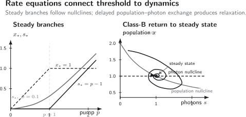
Left: in the low-$\beta$ model, the reservoir rises to $x=1$ and clamps while the photon number grows as $s=p-1$. Finite $\beta$ rounds the photon branch. Right: for a class-B laser above threshold, the population and photon nullclines intersect at a stable focus; their delayed exchange produces damped relaxation oscillations.

Steady-State Output

In the low-$\beta$ above-threshold branch,

$$n_* = n_s(p-1).$$

Using the definitions of $n_s$ and $p$,

$$\begin{aligned} n_* &= \frac{ R-R_{\mathrm{th}} }{ \kappa }, \\ \kappa n_* &= R-R_{\mathrm{th}}. \end{aligned}$$

The second equation is the excess-pump event balance. The total cavity loss rate consumes the stimulated photons created by pump events above threshold.

Through one output port,

$$\begin{aligned} P_{\mathrm{out}} &= \hbar\omega_\ell \kappa_{\mathrm{out}}n_* \\ &= \hbar\omega_\ell \frac{ \kappa_{\mathrm{out}} }{ \kappa } \left( R-R_{\mathrm{th}} \right). \end{aligned}$$

If incident pump power $P_p$ produces reservoir excitations with efficiency $\eta_p$,

$$R = \eta_p \frac{P_p}{\hbar\omega_p}.$$

The ideal differential optical efficiency is then

$$\frac{dP_{\mathrm{out}}}{dP_p} = \eta_p \frac{ \kappa_{\mathrm{out}} }{ \kappa } \frac{ \omega_\ell }{ \omega_p }.$$

This formula separates:

• pump absorption and transfer, $\eta_p$;
• useful output coupling, $\kappa_{\mathrm{out}}/\kappa$;
• the quantum defect, $\omega_\ell/\omega_p$.

Real slope efficiencies can be lower because mode overlap, excited-state absorption, reabsorption, thermal effects, and pump-dependent losses are not in the minimal model.

Output coupling is not free

Increasing $\kappa_{\mathrm{out}}$ extracts a larger fraction of each intracavity photon flux, but it also raises the total $\kappa$ and therefore

$$N_{\mathrm{th}} = \frac{\kappa}{g}.$$

An output coupler is optimized by solving both effects together. Holding $N_{\mathrm{th}}$ fixed while varying $\kappa_{\mathrm{out}}$ violates the model’s own threshold condition.

Relaxation Oscillations

Linearize above threshold

Take $\beta\simeq0$ and $p>1$. Write

$$x = 1+\delta x, \qquad s = p-1+\delta s.$$

To first order,

$$\frac{d}{dt} \begin{pmatrix} \delta x\\ \delta s \end{pmatrix} = \begin{pmatrix} -\gamma_N p & -\gamma_N\\ \kappa(p-1) & 0 \end{pmatrix} \begin{pmatrix} \delta x\\ \delta s \end{pmatrix}.$$

The characteristic equation is

$$\lambda^2 + \gamma_Np\,\lambda + \gamma_N\kappa(p-1) = 0.$$

Define the undamped relaxation scale and amplitude damping rate by

$$\begin{aligned} \omega_R^2 &= \gamma_N\kappa(p-1), \\ \Gamma_R &= \frac{\gamma_Np}{2}. \end{aligned}$$

The actual damped oscillation frequency is

$$\Omega_R = \sqrt{ \omega_R^2-\Gamma_R^2 }.$$

Underdamped relaxation oscillations occur when $\omega_R>\Gamma_R$. Otherwise the fixed point is approached without oscillation.

Physical mechanism

The oscillation is an exchange delayed by two finite response times:

1. a pump perturbation raises $N$;
2. gain exceeds loss, so $n$ grows rapidly;
3. stimulated emission depletes $N$ below its steady value;
4. photon loss then reduces $n$;
5. the pump rebuilds $N$.

The trajectory circles the intersection of the population and photon nullclines. Cavity leakage and population relaxation contract the orbit. These are not Rabi oscillations: the optical polarization has already been eliminated, and no coherent atom–field exchange appears in the model.

General differential-gain form

For an arbitrary smooth gain law, let

$$G(N_*) = \kappa, \qquad G'_* = \left. \frac{dG}{dN} \right|_{N_*}.$$

Linearization about a low-$\beta$ above-threshold state gives

$$\lambda^2 + \left( \gamma_N+G'_*n_* \right)\lambda + \kappa G'_*n_* = 0.$$

Thus

$$\begin{aligned} \omega_R^2 &= \kappa G'_*n_*, \\ \Gamma_R &= \frac{ \gamma_N+G'_*n_* }{2}. \end{aligned}$$

Gain compression, carrier-dependent recombination, and transport modify both quantities.

Small-signal modulation

Let the normalized pump be

$$p(t) = p_0+\delta p(t),$$

with $p_0>1$. Eliminating $\delta x$ gives

$$\begin{aligned} \delta\ddot s &+ \gamma_Np_0\, \delta\dot s \\ &+ \gamma_N\kappa (p_0-1) \delta s \\ &= \gamma_N\kappa (p_0-1) \delta p. \end{aligned}$$

The response is resonantly enhanced near $\Omega_R$ when damping is weak. This relaxation resonance is useful for diagnosing laser parameters and limits the flat direct-modulation bandwidth of many class-B lasers.

Turn-on delay and spiking

Immediately after a pump step, the field may still be too weak to deplete the reservoir. Neglecting stimulated emission during that buildup gives

$$N(t) = \frac{R}{\gamma_N} \left( 1-e^{-\gamma_Nt} \right).$$

For $R>R_{\mathrm{th}}$, the reservoir first reaches threshold at

$$t_{\mathrm{th}} = -\frac{1}{\gamma_N} \ln \left( 1-\frac{R_{\mathrm{th}}}{R} \right).$$

Afterward the photon number grows from its spontaneous or injected seed. Strong inversion overshoot can produce a large first spike followed by damped relaxation oscillations. The formula above is only the reservoir buildup time; the observed optical delay also includes growth from the seed to a detectable photon number.

Laser Classes and Adiabatic Elimination

The semiclassical Maxwell–Bloch description contains three characteristic decay rates:

• field or energy loss, represented here by $\kappa$;
• polarization decay, $\gamma_\perp$;
• population decay, $\gamma_\parallel\simeq\gamma_N$.

The traditional classes summarize which variables can be eliminated:

Class	Typical hierarchy	Minimal dynamics
A	$\gamma_\perp,\gamma_\parallel\gg\kappa$	eliminate polarization and population; retain field or intensity
B	$\gamma_\perp\gg\kappa\gg\gamma_\parallel$	eliminate polarization; retain photons and population
C	comparable rates	retain field, polarization, and population

The inequalities are asymptotic guides, not sharp material labels. Many solid-state and semiconductor lasers are class B, where the two-variable rate equations naturally support relaxation oscillations. Class-C dynamics requires the optical polarization and can include coherent instabilities that the present equations cannot represent.

Optical Bloch Equations provides the canonical two-level coherence dynamics from which polarization elimination can be understood.

Worked Example

Consider an effective four-level laser with

$$\begin{aligned} \gamma_N &= 4.00\times10^3\ \mathrm{s}^{-1}, \\ \kappa &= 2.00\times10^7\ \mathrm{s}^{-1}, \\ n_s &= 2.00\times10^8. \end{aligned}$$

Let the pump be $p=2.50$, take $\beta\ll1$, and suppose one useful output port accounts for one quarter of the cavity decay:

$$\kappa_{\mathrm{out}} = 0.25\kappa.$$

The steady normalized photon number is

$$s_* = p-1 = 1.50,$$

so

$$n_* = s_*n_s = 3.00\times10^8.$$

At $\lambda_\ell=1064\ \mathrm{nm}$,

$$\begin{aligned} P_{\mathrm{out}} &= \frac{hc}{\lambda_\ell} \kappa_{\mathrm{out}}n_* \\ &\simeq 2.80\times10^{-4}\ \mathrm W. \end{aligned}$$

The relaxation scale is

$$\begin{aligned} \omega_R &= \sqrt{ \gamma_N\kappa(p-1) } \\ &\simeq 3.46\times10^5\ \mathrm{s}^{-1}, \end{aligned}$$

or

$$f_R = \frac{\omega_R}{2\pi} \simeq 55.1\ \mathrm{kHz}.$$

The damping rate is

$$\Gamma_R = \frac{\gamma_Np}{2} = 5.00\times10^3\ \mathrm{s}^{-1}.$$

Because $\Gamma_R\ll\omega_R$, the turn-on transient is strongly underdamped. The linearized oscillation envelope decays on a scale $1/\Gamma_R=200\ \mu\mathrm s$.

Extensions and Boundaries

Three-level and quasi-three-level media

Retain at least upper- and lower-level populations when lower-state occupation causes reabsorption. The gain is a weighted inversion, and pump depletion may enter explicitly. Replacing all of that by $G(N)=gN$ can underestimate threshold and mispredict clamping.

Semiconductor lasers

Carrier-density models commonly use

$$\begin{aligned} \dot N &= \frac{\eta_i I}{q} - R_{\mathrm{rec}}(N) - G(N)S, \\ \dot S &= \Gamma G(N)S - \frac{S}{\tau_p} + \Gamma\beta R_{\mathrm{sp}}(N). \end{aligned}$$

Transparency density, confinement factor $\Gamma$, nonlinear recombination, gain compression, carrier transport, and amplitude–phase coupling matter. This equation is a translation guide, not a full semiconductor-laser model. Semiconductor Lasers Overview owns the band-occupation, quasi-Fermi-level, device-threshold, and external-cavity physics needed to interpret its parameters.

Multiple modes

For modes $\mu$,

$$\dot n_\mu = \left[ G_\mu(\{N_j\})-\kappa_\mu \right]n_\mu + R_{\mathrm{sp},\mu}.$$

All modes couple through shared populations. Spatial or spectral hole burning requires several reservoir variables or a distributed $N(\mathbf r,\omega,t)$. A single total population cannot represent antiphase dynamics or local gain depletion.

Phase and quantum noise

Photon number alone has no optical phase. Add complex field amplitudes and Langevin forces for semiclassical amplitude and phase noise, or use a quantum master equation when photon statistics and few-emitter correlations matter. Photon Counting owns the measurement of photon statistics, while Input–Output Theory Overview connects intracavity dynamics to propagating output fields.

Strong coupling and coherent transients

If atomic polarization cannot follow adiabatically, the stimulated term $G(N)n$ is insufficient. Retain field amplitude, polarization, and inversion. Vacuum Rabi oscillations, self-induced transparency, and other coherent phenomena are outside population-only rate equations.

A Reliable Modeling Workflow

1. Choose reservoirs. State which level populations or carrier densities are dynamical.
2. Choose one field convention. Use photon number, energy, intensity, or field amplitude consistently.
3. Write every event twice when appropriate. Stimulated emission must leave the material and enter the field with matching rates.
4. Separate useful and parasitic loss. Resolve $\kappa=\kappa_{\mathrm{out}}+\kappa_{\mathrm{other}}$.
5. Derive the gain law. Include transparency, overlap, and differential gain rather than importing an undefined coefficient.
6. Check the zero-field limit. Recover the independently pumped population dynamics.
7. Find all physical fixed points. Reject negative populations or photon numbers.
8. Linearize before interpreting transients. Eigenvalues distinguish monotonic return, damped relaxation, and instability.
9. Compare time scales. Decide whether polarization or population elimination is justified.
10. Escalate the model when observations demand it. Add modes, spatial bins, stochastic sources, or coherences only for identified physics.

Common Mistakes

Treating β as the coherent fraction

$\beta$ is a spontaneous-emission coupling fraction in the rate model. It does not say that a fraction $\beta$ of the output is coherent.

Calling every transient oscillation a Rabi oscillation

Relaxation oscillations exchange population and photon number after optical polarization has been eliminated. Rabi oscillations are coherent amplitude-level dynamics.

Mixing photon and field decay rates

If $a$ obeys $\dot a=-(\kappa_a)a$, then $n=|a|^2$ decays at $2\kappa_a$. State the defining equation for every linewidth or lifetime symbol.

Adding spontaneous photons without material depletion

The reservoir decay term already includes spontaneous decay. The field source $\beta\gamma_NN$ routes a fraction of those events into the selected mode; it does not create an independent energy source.

Inferring coherence from the mean curve

A smooth high-$\beta$ input–output curve and a low-$\beta$ kink are intensity features. Coherence and statistics require their own observables.

Holding threshold fixed while changing output coupling

Changing $\kappa_{\mathrm{out}}$ changes total $\kappa$, threshold inversion, and threshold pump. Recompute the fixed point.

Fitting too many effective parameters

Several combinations of pump efficiency, mode overlap, differential gain, and loss can generate similar mean curves. Use ringdown, spectroscopy, transients, and calibrated pump absorption to break degeneracies.

Exercises

1. Audit the stimulated event

Add the two minimal rate equations and explain which terms cancel. What physical quantity is conserved by stimulated emission in the idealized event ledger?

Solution

Adding gives

$$\frac{d}{dt}(N+n) = R - (1-\beta)\gamma_NN - \kappa n.$$

The terms $-G(N)n$ and $+G(N)n$ cancel. A stimulated event conserves the sum of effective reservoir excitations and cavity photons: it converts one of the former into one of the latter.

The remaining terms are external pump, reservoir decay into unmodeled channels, and cavity leakage. Energy rather than event-number conservation would additionally weight pump and laser excitations by their different frequencies.

2. Recover the normalized equations

Starting from $G(N)=gN$, substitute

$$x=\frac{N}{N_{\mathrm{th}}}, \qquad s=\frac{n}{n_s}, \qquad p=\frac{R}{R_{\mathrm{th}}},$$

and derive the normalized model.

Solution

Use

$$\begin{aligned} N_{\mathrm{th}} &= \frac{\kappa}{g}, \\ R_{\mathrm{th}} &= \gamma_NN_{\mathrm{th}}, \\ n_s &= \frac{\gamma_N}{g}. \end{aligned}$$

Then

$$\begin{aligned} \dot x &= \frac{1}{N_{\mathrm{th}}} \left( R-\gamma_NN-gNn \right) \\ &= \gamma_N(p-x-xs), \end{aligned}$$

and

$$\begin{aligned} \dot s &= \frac{1}{n_s} \left[ (gN-\kappa)n + \beta\gamma_NN \right] \\ &= \kappa \left[ (x-1)s+\beta x \right]. \end{aligned}$$

Every term now has units of inverse time times a dimensionless variable.

3. Test stability below threshold

For $\beta=0$, linearize around $x_*=p$, $s_*=0$. Determine when that fixed point is stable.

Solution

The Jacobian is

$$J_{\mathrm{off}} = \begin{pmatrix} -\gamma_N & -\gamma_Np\\ 0 & \kappa(p-1) \end{pmatrix}.$$

Its eigenvalues are the diagonal entries:

$$\lambda_1=-\gamma_N, \qquad \lambda_2=\kappa(p-1).$$

Both are negative only for $p<1$. At $p=1$, the photon-direction eigenvalue vanishes, and for $p>1$ the nonlasing state is unstable.

4. Evaluate the finite-β crossover

At $p=1$ and $\beta=10^{-2}$, find $s_*$ and $x_*$. Compare with the low-$\beta$ limiting branch.

Solution

At $p=1$,

$$s_*=\sqrt{\beta}=0.100.$$

Then

$$x_* = \frac{s_*}{s_*+\beta} = \frac{0.100}{0.110} \simeq 0.909.$$

The strict $\beta=0$ model meets the below- and above-threshold branches at $s_*=0$, $x_*=1$. Finite spontaneous feeding produces a nonzero mean photon number and slightly depletes the reservoir before that nominal pump value.

5. Derive the slope efficiency

Let

$$R = \eta_p \frac{P_p}{\hbar\omega_p}$$

and assume the low-$\beta$ above-threshold branch. Derive the differential output efficiency through a port with decay rate $\kappa_{\mathrm{out}}$.

Solution

Above threshold,

$$n_* = \frac{R-R_{\mathrm{th}}}{\kappa}.$$

Therefore

$$P_{\mathrm{out}} = \hbar\omega_\ell \frac{\kappa_{\mathrm{out}}}{\kappa} \left( R-R_{\mathrm{th}} \right).$$

If the model parameters are pump independent,

$$\frac{dP_{\mathrm{out}}}{dP_p} = \eta_p \frac{\kappa_{\mathrm{out}}}{\kappa} \frac{\omega_\ell}{\omega_p}.$$

The result is dimensionless and cannot exceed unity when all three factors represent passive efficiencies and a Stokes-shifted laser.

6. Classify the worked example

Use the worked-example parameters to compute $\Omega_R$ rather than $\omega_R$. How important is the damping correction?

Solution

The values are

$$\begin{aligned} \omega_R &\simeq 3.464\times10^5\ \mathrm{s}^{-1}, \\ \Gamma_R &= 5.00\times10^3\ \mathrm{s}^{-1}. \end{aligned}$$

Hence

$$\begin{aligned} \Omega_R &= \sqrt{ \omega_R^2-\Gamma_R^2 } \\ &\simeq 3.464\times10^5\ \mathrm{s}^{-1}. \end{aligned}$$

The fractional correction is approximately

$$\frac{ \omega_R-\Omega_R }{ \omega_R } \simeq 1.04\times10^{-4}.$$

The system is strongly underdamped, consistent with class-B behavior.

7. Estimate a turn-on delay

A pump step sets $R=3R_{\mathrm{th}}$ in a laser with $\tau_N=250\ \mu\mathrm s$. Estimate the time at which the un-depleted reservoir first reaches threshold.

Solution

Using $\gamma_N=1/\tau_N$,

$$\begin{aligned} t_{\mathrm{th}} &= -\tau_N \ln \left( 1-\frac{1}{3} \right) \\ &= -(250\ \mu\mathrm s) \ln\left(\frac{2}{3}\right) \\ &\simeq 101\ \mu\mathrm s. \end{aligned}$$

This excludes the additional photon buildup from the spontaneous seed to the detector threshold.

8. Choose the missing physics

A laser shows two longitudinal peaks whose intensities oscillate in opposition while their sum is nearly constant. Explain why the one-mode model fails and state a minimal extension.

Solution

One photon variable cannot represent redistribution between two modes. The nearly constant total intensity also suggests competition through a shared gain reservoir rather than a simple total-power instability.

A first extension uses $n_1$, $n_2$, and at least one shared population:

$$\begin{aligned} \dot N ={}& R-\gamma_NN \\ &- G_1(N)n_1 - G_2(N)n_2, \\ \dot n_\mu &= \left[ G_\mu(N)-\kappa_\mu \right]n_\mu + R_{\mathrm{sp},\mu}. \end{aligned}$$

If that model cannot reproduce the antiphase dynamics, add spatial or spectral population classes so each mode burns a different part of the gain distribution.

References

1. H. Statz and G. deMars, “Transients and Oscillation Pulses in Masers,” in C. H. Townes, ed., Quantum Electronics, Columbia University Press, pp. 530–537 (1960).
2. C. L. Tang, H. Statz, and G. deMars, “Spectral Output and Spiking Behavior of Solid-State Lasers,” Journal of Applied Physics 34, 2289–2295 (1963).
3. R. Dunsmuir, “Theory of Relaxation Oscillations in Optical Masers,” Journal of Electronics and Control 10, 453–458 (1961).
4. W. E. Lamb Jr., “Theory of an Optical Maser,” Physical Review 134, A1429–A1450 (1964).
5. M. O. Scully and W. E. Lamb Jr., “Quantum Theory of an Optical Maser. I. General Theory,” Physical Review 159, 208–226 (1967).
6. G. Björk and Y. Yamamoto, “Analysis of Semiconductor Microcavity Lasers Using Rate Equations,” IEEE Journal of Quantum Electronics 27, 2386–2396 (1991).
7. Y. Yamamoto, S. Machida, and G. Björk, “Microcavity Semiconductor Laser with Enhanced Spontaneous Emission,” Physical Review A 44, 657–668 (1991).
8. P. R. Rice and H. J. Carmichael, “Photon Statistics of a Cavity-QED Laser: A Comment on the Laser–Phase-Transition Analogy,” Physical Review A 50, 4318–4329 (1994).
9. H. Haken, “Cooperative Phenomena in Systems Far from Thermal Equilibrium and in Nonphysical Systems,” Reviews of Modern Physics 47, 67–121 (1975).
10. A. E. Siegman, Lasers, University Science Books (1986).
11. O. Svelto, Principles of Lasers, 5th ed., Springer (2010), doi:10.1007/978-1-4419-1302-9.
12. P. W. Milonni and J. H. Eberly, Laser Physics, Wiley (2010), doi:10.1002/9780470409718.
13. H. Haken, Laser Theory, Springer (1984), doi:10.1007/978-3-642-45551-7.
14. M. Sargent III, M. O. Scully, and W. E. Lamb Jr., Laser Physics, Addison–Wesley (1974).