Laser Principles

The basic laser problem is a nonlinear self-consistency problem:

After one circuit through gain, propagation, reflection, loss, and output coupling, can a field reproduce itself?

The answer has a magnitude part and a phase part. A weak field must return with at least its original magnitude, and it must return with the phase and spatial profile of a resonator mode. At the onset of oscillation, unsaturated gain exactly balances loss. Above onset, the field grows until it changes the medium enough that saturated gain again balances loss.

This yields the shortest useful chain of laser principles:

$$\begin{gathered} \text{pump} \longrightarrow \text{nonequilibrium medium} \\ \longrightarrow \text{net optical gain}, \\ \text{gain} + \text{feedback} + \text{phase selection} \\ \longrightarrow \text{oscillation}, \\ \text{oscillation} + \text{saturation} + \text{output loss} \\ \longrightarrow \text{steady laser output}. \end{gathered}$$

Every real architecture adds detail, but none can omit energy supply, mode selection, loss, and nonlinear regulation.

Canonical Scope

This page owns the first system-level quantitative model of a laser:

1. absorption, spontaneous emission, and stimulated emission as distinct material processes;
2. conversion from microscopic population imbalance to a propagation-gain coefficient;
3. a nonlinear field or intensity map over one resonator round trip;
4. threshold as loss of stability of the zero-field solution;
5. saturation as the mechanism that creates a finite operating point;
6. output coupling as both useful extraction and cavity loss;
7. the approximation ledger needed to use these formulas responsibly.

Several ingredients are imported rather than rederived:

• Stimulated Emission owns the $n+1$ mode factor, cross-section derivation, gain bandwidth, homogeneous saturation derivation, and amplifier-noise limit.
• Einstein Coefficients owns spectral-density conventions, degeneracy relations, and thermal detailed balance.
• Spontaneous Emission owns vacuum-continuum dynamics and radiative decay.
• Optical Bloch Equations own coherent saturation, dephasing, and power broadening.
• Input–Output Theory Overview owns quantum traveling-field boundary conditions and output noise.

Population Inversion owns detailed pumping architectures and the two-, three-, and four-level population logic. Gain and Threshold owns nonuniform modal gain and complete loss budgets. The other pages that follow own rate equations, resonator geometry, mode locking, frequency combs, semiconductor devices, and stabilization. Linewidth and Coherence owns the stochastic phase dynamics omitted from this deterministic round-trip model. This page deliberately uses one uniform, single-mode, steady-state model as the first solvable case.

System Boundary and Conventions

The model is a linear optical cavity containing a pumped gain region of one-way length $L$. The field crosses that region twice per round trip. Mirror 1 is the high reflector and mirror 2 is the output coupler.

Use:

• $R_j=|r_j|^2$ for mirror power reflectivities;
• $T_j=|t_j|^2$ for power transmissivities;
• $g(\omega,I)$ for material power gain per unit length;
• $\alpha_{\mathrm i}$ for distributed internal power loss per unit length;
• $\ell$ for any additional lumped round-trip power survival factor;
• $\Phi_{\mathrm{rt}}(\omega,I)$ for round-trip phase;
• $I_m$ for intensity at a declared reference plane after round trip $m$;
• $\mathcal G_{\mathrm{rt}}(I)$ for the deterministic round-trip power multiplier;
• $I_{\mathrm{sat}}$ for the saturation intensity in the declared material model;
• $P_{\mathrm{circ}}$ for power incident on the output coupler from inside;
• $P_{\mathrm{out}}$ for useful transmitted output power.

The distinction between power and field matters:

$$I \propto |\mathcal E|^2.$$

If a device multiplies field amplitude by $a$, it multiplies power by $|a|^2$. Gain coefficients are also convention dependent. This page defines $g$ through the power equation

$$\frac{dI}{dz} = gI$$

before loss is added. An amplitude equation therefore contains $g/2$.

Absorption and Emission

Consider lower and upper material levels $1$ and $2$, with

$$E_2-E_1 = \hbar\omega_0 > 0.$$

Three radiative processes enter the elementary rate picture:

Process	Material change	Dependence on resonant radiation
absorption	$1\to2$	proportional to field occupation or spectral energy density
stimulated emission	$2\to1$	proportional to field occupation or spectral energy density
spontaneous emission	$2\to1$	remains when the receiving modes are initially empty

For an isotropic spectral energy density $u(\nu)$, Einstein’s rate description is

$$\begin{aligned} \mathcal R_{\mathrm{abs}} &= \mathcal N_1B_{12}u(\nu), \\ \mathcal R_{\mathrm{stim}} &= \mathcal N_2B_{21}u(\nu), \\ \mathcal R_{\mathrm{sp}} &= \mathcal N_2A_{21}. \end{aligned}$$

Here $\mathcal N_i$ are level populations per unit volume. The relation

$$g_1B_{12} = g_2B_{21}$$

contains the level degeneracies $g_1$ and $g_2$. A common mistake is to set $B_{12}=B_{21}$ before checking degeneracy conventions.

These rates do not yet describe a collimated laser mode. Converting from isotropic energy density to beam intensity requires a declared angular, polarization, and lineshape normalization. Effective absorption and emission cross sections are more convenient for propagation.

Net stimulated energy transfer

For a photon flux

$$\Phi_\gamma = \frac{I}{\hbar\omega},$$

write the stimulated rates per active particle as

$$W_a = \sigma_a(\omega)\Phi_\gamma, \qquad W_e = \sigma_e(\omega)\Phi_\gamma.$$

The net stimulated event rate per unit volume is

$$\mathcal R_{\mathrm{net}} = \Phi_\gamma \left[ \sigma_e(\omega)\mathcal N_2 - \sigma_a(\omega)\mathcal N_1 \right].$$

The bracket is the small-signal material gain coefficient:

$$g_0(\omega) = \sigma_e(\omega)\mathcal N_2 - \sigma_a(\omega)\mathcal N_1.$$

Positive $g_0$ means that the selected weak beam extracts more energy through stimulated emission than it loses through absorption. It does not mean the device has reached laser threshold; cavity and propagation losses have not yet been included.

The inversion condition

If the two effective cross sections are equal,

$$\sigma_e = \sigma_a = \sigma,$$

then

$$g_0 = \sigma \left( \mathcal N_2-\mathcal N_1 \right),$$

and positive gain requires population inversion. With degeneracy, reabsorption, Stark or Zeeman substructure, thermalized manifolds, or unequal lineshapes, the threshold population condition changes. The invariant criterion is positive net gain for the actual mode.

Thermal equilibrium at positive temperature cannot provide ordinary optical gain on an isolated transition. Pumping must establish a nonequilibrium population or coherence. The detailed reason a closed two-level system does not sustain inversion, and the construction of three- and four-level schemes, belongs to the dedicated population-inversion treatment.

From Material Response to Gain

Traveling-wave amplification

For weak intensity and uniform coefficients,

$$\frac{dI}{dz} = \left[ g_0(\omega) - \alpha_{\mathrm i} \right]I.$$

The one-pass solution is

$$I(L) = I(0) \exp \left\{ \left[ g_0(\omega)-\alpha_{\mathrm i} \right]L \right\}.$$

The dimensionless power gain is therefore

$$G_{\mathrm{pass}} = \frac{I(L)}{I(0)}.$$

It should not be confused with $g_0$, which has dimensions of inverse length. A report of “gain 3” is ambiguous unless it says whether this is an amplitude ratio, power ratio, or logarithmic gain.

For power gain,

$$G_{\mathrm{dB}} = 10\log_{10}G_{\mathrm{pass}}.$$

For a field-amplitude ratio, the equivalent expression is $20\log_{10}|a|$.

Modal gain

A cavity mode generally overlaps only part of the pumped region. A simple confinement or overlap factor $\Gamma$ gives

$$g_{\mathrm{modal}} = \Gamma g_{\mathrm{material}}, \qquad 0\le\Gamma\le1.$$

In a realistic model, $\Gamma$ can include transverse mode shape, longitudinal standing-wave structure, polarization, and spatially varying inversion. A high local material gain is useless to a mode that barely overlaps it.

Gain bandwidth and dispersion

Gain is complex at the field level. Its imaginary and real response parts are linked by causality, so amplification comes with dispersion. A field must lie inside the gain bandwidth and satisfy the cavity phase condition after that dispersion is included.

The frequency of maximum material gain need not equal a cold-cavity resonance. Oscillation occurs where the combined modal gain, loss, and phase conditions are met. Pump-induced heating and population changes can shift all three.

Spontaneous source term

The homogeneous propagation equation omits light generated within the medium. A radiative-transfer form is

$$\frac{dI}{dz} = \left( g-\alpha_{\mathrm i} \right)I + j_{\mathrm{sp}},$$

where $j_{\mathrm{sp}}$ is a mode-, bandwidth-, and solid-angle-dependent source term. Below laser threshold this term produces amplified spontaneous emission. Near threshold it also seeds the cavity modes and rounds the otherwise sharp deterministic onset.

Feedback as a Round-Trip Map

Choose one reference plane in the cavity and one candidate mode. Its complex field amplitude after successive round trips can be represented as

$$\mathcal E_{m+1} = \mathcal A_{\mathrm{rt}} \left( \omega, |\mathcal E_m|^2 \right) e^{i\Phi_{\mathrm{rt}}} \mathcal E_m + \xi_m.$$

The complex multiplier $\mathcal A_{\mathrm{rt}}$ contains gain and loss. The phase $\Phi_{\mathrm{rt}}$ contains propagation, reflection, and dispersive phase. The fluctuation $\xi_m$ represents spontaneous emission and other noise coupled into the mode.

This one equation separates three questions:

1. Magnitude: is $|\mathcal A_{\mathrm{rt}}|$ smaller or larger than one for a weak field?
2. Phase: does the field return with a self-consistent phase?
3. Nonlinearity: how does the multiplier change as the field saturates the medium?

Deterministic power map

Suppress noise temporarily and define

$$I_{m+1} = F(I_m) = \mathcal G_{\mathrm{rt}}(I_m)I_m.$$

For the uniform linear cavity,

$$\mathcal G_{\mathrm{rt}}(I) = \ell R_1R_2 \exp \left\{ 2 \left[ g(I)-\alpha_{\mathrm i} \right]L \right\}.$$

The lumped survival factor $\ell$ can include windows, apertures, filters, and other discrete power losses. If each element has survival $\ell_j$, then

$$\ell = \prod_j\ell_j.$$

Every factor must refer to the same complete round trip. Omitting a second pass through the gain medium or counting a mirror twice changes the threshold.

Resonance phase

A self-reproducing field also obeys

$$\Phi_{\mathrm{rt}}(\omega) = 2\pi q, \qquad q\in\mathbb Z.$$

For an empty nondispersive linear cavity of optical length $L_{\mathrm{opt}}$,

$$\nu_q \simeq \frac{qc}{2L_{\mathrm{opt}}}, \qquad \Delta\nu_{\mathrm{FSR}} \simeq \frac{c}{2L_{\mathrm{opt}}}.$$

The longitudinal mode index is normally enormous at optical frequencies. Only the mode spacing and offsets are directly convenient. Gain dispersion and mirror phase shift the resonances from this empty-cavity estimate. Optical Cavities derives the group-delay free spectral range, Airy response, spatial stability, and transverse-mode scales without the empty-cavity approximations used here.

A mode is an eigenfunction

The scalar map assumes that propagation returns the same spatial and polarization pattern times one complex number. More generally, one round trip is an operator $\mathcal R$ acting on a field profile:

$$\mathcal R u_\mu = \lambda_\mu u_\mu.$$

The candidate laser modes $u_\mu$ are eigenfunctions of the complete round-trip problem, including apertures, gain guiding, lenses, diffraction, and polarization optics. Threshold is reached first by the eigenmode whose net round-trip magnitude reaches unity under the available pump.

This is why “two parallel mirrors select a frequency” is incomplete. A laser mode is jointly spatial, spectral, and polarizational. Laser Modes develops the normalized HG and LG eigenfamilies, mode measurements, beam quality, and nonlinear competition that this first round-trip model leaves implicit.

Threshold

Linearize the deterministic map around the empty solution:

$$I_{m+1} \simeq \mathcal G_{\mathrm{rt}}(0)I_m.$$

The zero-field solution is stable when

$$\mathcal G_{\mathrm{rt}}(0) < 1$$

and unstable when

$$\mathcal G_{\mathrm{rt}}(0) > 1.$$

The small-signal threshold is therefore

$$\mathcal G_{\mathrm{rt}}(0) = 1.$$

For $\ell=1$, this gives

$$\begin{aligned} g_{\mathrm{th}} ={}& \alpha_{\mathrm i} \\ &+ \frac{1}{2L} \ln \left( \frac{1}{R_1R_2} \right). \end{aligned}$$

With a lumped survival factor,

$$\begin{aligned} g_{\mathrm{th}} ={}& \alpha_{\mathrm i} \\ &+ \frac{1}{2L} \ln \left( \frac{1}{ \ell R_1R_2 } \right). \end{aligned}$$

These are material power-gain coefficients for the stated uniform model. If $g$ is modal gain, the overlap is already included. If $g$ is material gain, the threshold condition must use $\Gamma g$.

Threshold inversion

Under the restrictive equal-cross-section model,

$$g_0 = \sigma\Delta\mathcal N, \qquad \Delta\mathcal N = \mathcal N_2-\mathcal N_1.$$

The threshold inversion density is

$$\Delta\mathcal N_{\mathrm{th}} = \frac{g_{\mathrm{th}}}{\sigma}.$$

This is not yet a pump threshold. Converting inversion into pump power requires level kinetics, pump absorption, active volume, quantum efficiency, branching, and thermal losses.

Growth time just above threshold

Let the round-trip time be $t_{\mathrm{rt}}$. If

$$\mathcal G_{\mathrm{rt}}(0) = 1+\epsilon, \qquad 0<\epsilon\ll1,$$

then after $m$ round trips

$$I_m \simeq (1+\epsilon)^mI_0 \simeq e^{m\epsilon}I_0.$$

Since $t=mt_{\mathrm{rt}}$, the initial power growth rate is approximately

$$\gamma_{\mathrm{build}} \simeq \frac{\epsilon}{t_{\mathrm{rt}}}.$$

Near threshold the build-up can therefore be slow even though net gain is positive. Population dynamics and spontaneous seeding set the actual turn-on transient.

Saturation and the Operating Fixed Point

Linear gain cannot describe steady lasing. If $\mathcal G_{\mathrm{rt}}>1$ remained constant, the model would predict unbounded field growth. The field must reduce the available gain or activate another nonlinear loss.

For a simple homogeneously broadened steady-state medium, import the constitutive model

$$g(I) = \frac{g_0}{ 1+I/I_{\mathrm{sat}} }.$$

Its derivation and limits are given on Stimulated Emission. Here it closes the oscillator equation.

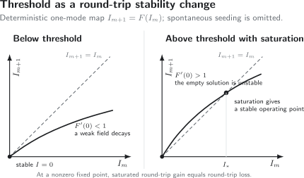
In the deterministic one-mode map $I_{m+1}=F(I_m)$, the slope at the origin is the small-signal round-trip multiplier. Below threshold the empty solution is stable. Above threshold it is unstable, while saturation bends the map toward a nonzero fixed point $I_*$. Spontaneous emission and technical noise blur both ideal fixed points in a physical device.

Gain clamping

At a nonzero steady state,

$$I_* = \mathcal G_{\mathrm{rt}}(I_*)I_*.$$

Because $I_*>0$,

$$\mathcal G_{\mathrm{rt}}(I_*) = 1.$$

In the uniform cavity this is equivalent to

$$g(I_*) = g_{\mathrm{th}}.$$

The gain seen by the oscillating mode is therefore clamped to threshold gain in this steady model. The unsaturated gain $g_0$ may be larger, but the field depletes the inversion until the saturated value balances loss.

Substituting the homogeneous saturation law gives

$$\frac{g_0}{ 1+I_*/I_{\mathrm{sat}} } = g_{\mathrm{th}}.$$

Hence

$$I_* = I_{\mathrm{sat}} \left( \frac{g_0}{g_{\mathrm{th}}} - 1 \right), \qquad g_0>g_{\mathrm{th}}.$$

This compact result is the first input–output law of the model. It assumes that $I$ is the same intensity used to define $I_{\mathrm{sat}}$, that gain is uniform, and that one mode alone saturates the medium.

Stability of the finite solution

For a discrete map, a fixed point is locally stable if

$$\left| F'(I_*) \right| < 1.$$

Since

$$F(I) = \mathcal G_{\mathrm{rt}}(I)I,$$

one has

$$F'(I_*) = 1 + I_* \mathcal G_{\mathrm{rt}}'(I_*).$$

Ordinary gain saturation makes $\mathcal G_{\mathrm{rt}}'(I_*)<0$, providing negative feedback. This one-variable criterion does not capture population delay, relaxation oscillations, saturable absorbers, or multimode instabilities; those require a dynamical state larger than $I$ alone.

Mode competition

If several modes draw on one homogeneous inversion, the saturation produced by one changes the gain available to the others. The first mode to reach threshold can suppress competitors. Inhomogeneous broadening, spatial hole burning, polarization structure, and separate gain reservoirs weaken that competition and can support multimode operation.

Gain clamping is therefore mode and location dependent. It does not imply that every point in a real gain medium or every frequency in its bandwidth has exactly threshold gain.

Output Coupling

An ideal laser would be useless if no field escaped. The output coupler deliberately converts part of the intracavity mode into a traveling beam.

At a declared plane immediately before the coupler,

$$P_{\mathrm{out}} = T_2P_{\mathrm{circ}},$$

when mode matching is perfect and $T_2$ denotes useful transmission. If the mirror also absorbs or scatters,

$$R_2+T_2+A_2 = 1.$$

Only $T_2$ is useful output, whereas both $T_2$ and $A_2$ contribute to cavity loss.

Escape efficiency

For small per-round-trip losses, let $L_{\mathrm i}$ be the sum of all internal parasitic power losses and let $T$ be the intended output transmission. The fraction of cavity-decay events leaving through the useful port is approximately

$$\eta_{\mathrm{esc}} \simeq \frac{T}{ T+L_{\mathrm i} }.$$

This ratio is a branching fraction for stored optical energy. It is not the wall-plug efficiency and does not include pump absorption, quantum defect, fluorescence into unwanted modes, heat, electronics, or mode mismatch.

The output-coupling tradeoff

Increasing $T$ has two opposing effects:

1. a larger fraction of circulating power exits on each encounter;
2. threshold rises, saturation changes, and circulating power can fall.

If $T$ is too small, internal losses consume much of the generated power and little useful light escapes. If $T$ is too large, available gain may be insufficient to reach threshold. The optimum depends on pump level, saturated gain, internal loss, active-mode overlap, and the desired operating regime.

“Use the most reflective mirror possible” and “extract as much as possible” are both incomplete design rules.

Slope efficiency

Above threshold, output power often becomes approximately linear in absorbed pump power over a limited range:

$$P_{\mathrm{out}} \simeq \eta_s \left( P_{\mathrm p} - P_{\mathrm{th}} \right).$$

The slope efficiency $\eta_s$ is local to that operating range. It contains pump absorption, energy conversion, spatial overlap, internal loss, output coupling, and other architecture-specific factors. It is not generally equal to the optical escape efficiency.

Worked Operating-Point Example

Take a uniform linear cavity with

$$\begin{gathered} L=0.12\ \mathrm m, \qquad R_1=0.999, \\ R_2=0.960, \qquad \alpha_{\mathrm i}=0.015\ \mathrm{m}^{-1}. \end{gathered}$$

Ignore other lumped losses. The threshold material power gain is

$$\begin{aligned} g_{\mathrm{th}} &= 0.015 + \frac{1}{0.24} \ln \left[ \frac{1}{ (0.999)(0.960) } \right] \\ &\simeq 0.189\ \mathrm{m}^{-1}. \end{aligned}$$

Suppose the pumped small-signal gain and saturation intensity are

$$g_0 = 0.280\ \mathrm{m}^{-1}, \qquad I_{\mathrm{sat}} = 2.50\ \mathrm{kW\,m^{-2}}.$$

The one-mode fixed-point model predicts

$$\begin{aligned} I_* &= I_{\mathrm{sat}} \left( \frac{g_0}{g_{\mathrm{th}}} - 1 \right) \\ &\simeq 1.20\ \mathrm{kW\,m^{-2}}. \end{aligned}$$

For an effective beam area

$$A_{\mathrm{eff}} = 0.50\ \mathrm{mm^2},$$

the corresponding circulating power at the chosen reference plane is

$$P_{\mathrm{circ}} = I_*A_{\mathrm{eff}} \simeq 0.60\ \mathrm W.$$

If the output coupler is lossless so that $T_2=1-R_2=0.040$, then

$$P_{\mathrm{out}} = T_2P_{\mathrm{circ}} \simeq 24\ \mathrm{mW}.$$

The arithmetic is internally consistent, but the physical interpretation is only as good as the model. A standing-wave intensity varies along the gain medium; Gaussian intensity varies across it; gain may not be uniform; and the effective area used in a saturation law depends on its definition. This example is a consistency check, not a universal laser-design formula.

Energy and Information Flow

It helps to keep two ledgers.

Energy ledger

Pump energy can become:

• stored material excitation;
• useful laser output;
• spontaneous fluorescence;
• amplified spontaneous emission;
• nonradiative heat;
• residual pump transmission;
• internal absorption and scattering.

Stimulated emission transfers stored material energy to the selected field. It does not create energy and does not obtain the output photon energy from the stimulating photon.

Information and phase ledger

The output mode inherits its reproducible structure from:

• resonator boundary conditions;
• gain and loss spectra;
• pump geometry;
• polarization optics;
• nonlinear mode competition;
• initial fluctuations and continuing noise;
• any injected seed or stabilization reference.

The pump supplies energy but does not automatically fix the optical phase. In an unseeded free-running laser, continuous symmetry and noise permit phase diffusion. An injected field or feedback reference can select and stabilize a relative phase.

Approximation Ledger

The one-mode round-trip model is useful when:

Assumption	Meaning	Warning sign
one selected mode	other modes remain below threshold or are negligible	multiple spectral peaks or spatial patterns
uniform gain	one coefficient represents the active path	strong pump depletion or transverse gradients
steady saturation	material follows the field adiabatically	turn-on transients or relaxation oscillations
scalar polarization	one polarization eigenmode is isolated	birefringence, vector gain, polarization switching
lumped feedback	one round-trip map is sufficient	distributed feedback or strong propagation dynamics
weak noise	mean operating point is well defined	nanolaser, threshold statistics, excess technical noise
fixed temperature and geometry	cavity and medium are stationary	thermal lensing, drift, deformation

Several familiar effects signal the need for a larger model:

• relaxation oscillations: retain at least population and photon number, as derived in Rate-Equation Lasers;
• spatial hole burning: resolve longitudinal intensity and inversion;
• inhomogeneous saturation: resolve frequency or emitter classes;
• mode locking: retain many longitudinal modes and their phases, as developed in Mode Locking;
• Q switching: retain time-dependent loss and stored inversion;
• semiconductor dynamics: retain carrier densities, confinement, and amplitude–phase coupling;
• quantum statistics near threshold: retain the field density operator or stochastic quantum dynamics.

A Reliable Calculation Workflow

1. Choose the reference plane. State where $I$, $P_{\mathrm{circ}}$, and the round trip begin and end.
2. Choose power or amplitude variables. Do not mix $R$ with $r$ or $g$ with $g/2$.
3. Write the material constitutive law. Give populations, cross sections, lineshape, overlap, and saturation convention.
4. Inventory every loss. Separate useful output coupling from parasitic absorption, scattering, diffraction, and mode mismatch.
5. Impose magnitude and phase conditions. Positive one-pass gain is not oscillation.
6. Linearize for threshold. Use unsaturated gain and identify the leading round-trip eigenmode.
7. Solve the nonlinear fixed point. Verify that saturated gain balances loss and test local stability.
8. Convert to measured output. Apply the actual transmission, collection, detector response, and uncertainty.
9. Test limiting cases. Removing the pump must remove gain; removing feedback must leave an amplifier; removing saturation must expose unbounded growth and therefore model incompleteness.

Common Mistakes

Confusing positive gain with laser threshold

A single pass can amplify while the round-trip multiplier remains below one. Threshold concerns the complete feedback loop.

Counting gain or loss on the wrong number of passes

A linear cavity usually traverses the active region twice per round trip. A ring may traverse it once. Draw the path before writing the exponent.

Omitting the phase condition

Round-trip magnitude greater than one does not make every frequency grow. Only self-consistent resonator modes receive coherent feedback.

Applying small-signal gain above threshold

The unsaturated coefficient predicts onset. The steady oscillating mode sees saturated gain, which is clamped to net loss in the simple model.

Treating spontaneous emission as optional

It may be negligible in a mean above-threshold power balance, but it seeds unseeded oscillation and contributes unavoidable noise and linewidth.

Calling output coupling an external afterthought

The output coupler belongs inside the threshold condition because useful output is a cavity loss.

Equating escape efficiency and wall-plug efficiency

Escape efficiency describes where stored photons leave. Wall-plug efficiency includes the entire electrical, pump, material, thermal, and optical chain.

Assuming gain clamping is pointwise and universal

Spatially varying, multimode, or inhomogeneously broadened systems can retain unsaturated gain in regions or subensembles not depleted by the lasing mode.

Using a saturation intensity without its model

$I_{\mathrm{sat}}$ depends on transition, detuning, relaxation, polarization, line broadening, and whether peak, average, traveling-wave, or standing-wave intensity is meant.

Cross-Links

• Laser Nomenclature gives the compact convention checks for gain, threshold, resonator metrics, coherence, coherent driving, and saturation.
• Lasers is the chapter map for linewidth, pulses, combs, device classes, and AMO applications.
• Absorption and Emission connects material rates to measured source and transmission spectra.
• Line Shapes and Broadening develops homogeneous, inhomogeneous, natural, Doppler, collisional, and instrumental widths.
• Coherent Light explains when a propagating laser mode is well approximated by a coherent state.
• Cavity QED treats the regime in which individual emitters and a resonator exchange excitations coherently.

Exercises

1. Degeneracy and the gain condition

Two levels have degeneracies $g_1=2$ and $g_2=4$. Their Einstein coefficients obey $g_1B_{12}=g_2B_{21}$. Ignoring spontaneous emission in the stimulated power balance, what population ratio $\mathcal N_2/\mathcal N_1$ is required for positive gain?

Solution

The Einstein relation gives

$$B_{12} = \frac{g_2}{g_1}B_{21} = 2B_{21}.$$

Positive net stimulated emission requires

$$\mathcal N_2B_{21} > \mathcal N_1B_{12}.$$

Therefore

$$\frac{\mathcal N_2}{\mathcal N_1} > \frac{B_{12}}{B_{21}} = 2.$$

Equivalently, the population per magnetic sublevel must be inverted:

$$\frac{\mathcal N_2}{g_2} > \frac{\mathcal N_1}{g_1}.$$

2. Field gain versus power gain

A one-pass device has power gain $G_{\mathrm{pass}}=9$ and adds no phase shift. What is its field-amplitude gain? What is the power gain in decibels?

Solution

Because power is proportional to squared field amplitude,

$$\frac{\mathcal E_{\mathrm{out}}}{ \mathcal E_{\mathrm{in}} } = \sqrt{G_{\mathrm{pass}}} = 3.$$

The power gain in decibels is

$$\begin{aligned} G_{\mathrm{dB}} &= 10\log_{10}9 \\ &\simeq 9.54\ \mathrm{dB}. \end{aligned}$$

Using $20\log_{10}3$ gives the same numerical answer because 3 is the amplitude ratio.

3. Include a lumped intracavity loss

A linear cavity has $L=0.25\ \mathrm m$, $R_1=0.998$, $R_2=0.92$, $\alpha_{\mathrm i}=0.010\ \mathrm{m}^{-1}$, and an additional round-trip power survival $\ell=0.97$. Find the threshold material power gain.

Solution

Use

$$\begin{aligned} g_{\mathrm{th}} ={}& \alpha_{\mathrm i} \\ &+ \frac{1}{2L} \ln \left[ \frac{1}{ \ell R_1R_2 } \right]. \end{aligned}$$

The complete lumped survival is

$$\ell R_1R_2 = (0.97)(0.998)(0.92) \simeq 0.8906.$$

Thus

$$\begin{aligned} g_{\mathrm{th}} &= 0.010 + \frac{1}{0.50} \ln \left( \frac{1}{0.8906} \right) \\ &\simeq 0.242\ \mathrm{m}^{-1}. \end{aligned}$$

The factor $2L$ already accounts for two passes through the gain region.

4. Find the saturated operating intensity

A single-mode laser has $g_0=0.45\ \mathrm{m}^{-1}$, $g_{\mathrm{th}}=0.30\ \mathrm{m}^{-1}$, and $I_{\mathrm{sat}}=4.0\ \mathrm{kW\,m^{-2}}$. Use the homogeneous saturation law to find $I_*$. Verify the clamped gain.

Solution

The nonzero fixed point is

$$\begin{aligned} I_* &= I_{\mathrm{sat}} \left( \frac{g_0}{g_{\mathrm{th}}} - 1 \right) \\ &= (4.0\ \mathrm{kW\,m^{-2}}) (1.5-1) \\ &= 2.0\ \mathrm{kW\,m^{-2}}. \end{aligned}$$

At that intensity,

$$\begin{aligned} g(I_*) &= \frac{0.45}{ 1+2.0/4.0 } \\ &= 0.30\ \mathrm{m}^{-1} = g_{\mathrm{th}}. \end{aligned}$$

The saturated gain, not the unsaturated gain, balances cavity loss.

5. Estimate an initial build-up time

A candidate mode has round-trip time $t_{\mathrm{rt}}=2.0\ \mathrm{ns}$ and small-signal power multiplier $\mathcal G_{\mathrm{rt}}=1.004$. Estimate the initial $e$-folding time of power before saturation matters.

Solution

Here

$$\epsilon = \mathcal G_{\mathrm{rt}}-1 = 0.004.$$

The approximate growth rate is

$$\gamma_{\mathrm{build}} \simeq \frac{0.004}{ 2.0\ \mathrm{ns} } = 2.0\times10^6\ \mathrm{s}^{-1}.$$

Therefore

$$\tau_{\mathrm{build}} \simeq \gamma_{\mathrm{build}}^{-1} = 0.50\ \mu\mathrm s.$$

This is only the linear field build-up scale. Population evolution, spontaneous seeding, and changing gain can lengthen or shorten the observed turn-on transient.

6. Output and parasitic channels

A cavity loses $T=0.030$ of its power through the useful output port and $L_{\mathrm i}=0.010$ through all parasitic channels per round trip. Estimate the escape efficiency. If the circulating power incident on the output coupler is $8.0\ \mathrm W$, find the useful output at that encounter.

Solution

For small losses,

$$\eta_{\mathrm{esc}} \simeq \frac{0.030}{ 0.030+0.010 } = 0.75.$$

Three quarters of cavity-decay events leave through the intended channel in this approximation.

The directly transmitted output is

$$\begin{aligned} P_{\mathrm{out}} &= TP_{\mathrm{circ}} \\ &= (0.030)(8.0\ \mathrm W) \\ &= 0.24\ \mathrm W. \end{aligned}$$

The escape efficiency and the instantaneous output-coupling relation answer different questions.

7. Audit a round-trip map

A proposed model uses

$$I_{m+1} = 1.30 \frac{I_m}{ 1+I_m/I_s }.$$

Find its nonzero fixed point and determine whether the origin is stable.

Solution

The map is

$$F(I) = \frac{1.30I}{ 1+I/I_s }.$$

At the origin,

$$F'(0) = 1.30 > 1,$$

so the zero-intensity solution is unstable in the deterministic model.

For $I_*>0$,

$$1 = \frac{1.30}{ 1+I_*/I_s }.$$

Therefore

$$\frac{I_*}{I_s} = 0.30, \qquad I_* = 0.30I_s.$$

The saturating denominator creates the finite fixed point. A physical model would also include noise and material response time.

8. Design an evidence checklist

A datasheet describes a source as “single-mode, 1 MHz linewidth, 20% efficient laser output.” List the minimum clarifications needed before using those claims in a precision AMO calculation.

Solution

At minimum, ask:

1. whether single-mode refers to longitudinal, transverse, and polarization mode simultaneously;
2. how the linewidth was measured, over what observation time and Fourier-frequency range, with which FWHM or HWHM convention;
3. whether slow drift, modulation sidebands, and non-Lorentzian noise are included;
4. whether 20% is wall-plug, absorbed-pump, optical-to-optical, slope, or escape efficiency;
5. where output power and beam quality were measured;
6. how frequency, power, pointing, and polarization change with time, temperature, and tuning;
7. whether the stated operating point matches the intended experiment.

The labels become useful only after the observable and convention behind each number are known.

References

1. A. Einstein, “Zur Quantentheorie der Strahlung,” Physikalische Zeitschrift 18, 121–128 (1917).
2. A. L. Schawlow and C. H. Townes, “Infrared and Optical Masers,” Physical Review 112, 1940–1949 (1958).
3. T. H. Maiman, “Stimulated Optical Radiation in Ruby,” Nature 187, 493–494 (1960).
4. W. E. Lamb Jr., “Theory of an Optical Maser,” Physical Review 134, A1429–A1450 (1964).
5. M. O. Scully and W. E. Lamb Jr., “Quantum Theory of an Optical Maser. I. General Theory,” Physical Review 159, 208–226 (1967).
6. H. Kogelnik and T. Li, “Laser Beams and Resonators,” Applied Optics 5, 1550–1567 (1966).
7. A. E. Siegman, Lasers, University Science Books (1986).
8. O. Svelto, Principles of Lasers, 5th ed., Springer (2010), doi:10.1007/978-1-4419-1302-9.
9. P. W. Milonni and J. H. Eberly, Laser Physics, Wiley (2010), doi:10.1002/9780470409718.
10. M. Sargent III, M. O. Scully, and W. E. Lamb Jr., Laser Physics, Addison–Wesley (1974).
11. H. Haken, Laser Theory, Springer (1984), doi:10.1007/978-3-642-45551-7.
12. L. Mandel and E. Wolf, Optical Coherence and Quantum Optics, Cambridge University Press (1995), doi:10.1017/CBO9781139644105.